metamodel allowing to express the same kind of class models. Even for the ... Such model transformations are not difficult to write, but ... graphs are used in a fix-point computation process whose result tells us what ... We illustrate these three steps using the two metamodels exMMsource and ..... This common denominator.
Metamodel Matching for Automatic Model Transformation Generation? J.-R. Falleri1 , M. Huchard1 , M. Lafourcade1 , and C. Nebut1 LIRMM, CNRS and Universit´e de Montpellier 2, 161, rue Ada, 34392 Montpellier cedex 5, France {falleri, huchard, lafourcade, nebut}@lirmm.fr
Abstract. Applying Model-Driven Engineering (MDE) leads to the creation of a large number of metamodels, since MDE recommends an intensive use of models defined by metamodels. Metamodels with similar objectives are then inescapably created. A recurrent issue is thus to turn compatible models conforming to similar metamodels, for example to use them in the same tool. The issue is classically solved developing ad hoc model transformations. In this paper, we propose an approach that automatically detects mappings between two metamodels and uses them to generate an alignment between those metamodels. This alignment needs to be manually checked and can then be used to generate a model transformation. Our approach is built on the Similarity Flooding algorithm used in the fields of schema matching and ontology alignment. Experimental results comparing the effectiveness of the application of various implementations of this approach on real-world metamodels are given.
1
Introduction
The large success of Model-Driven Engineering leads to a relative abundance of metamodels, for various domains. Tools are developped to handle models conforming to the metamodels : code generators, model transformations and graphical editors. Inescapably, several metamodels for the same kind of applications are independently created. It is then quite natural to wish to use a tool-set adapted to a given metamodel for models conforming to another metamodel with the same purpose. For example, several metamodels exist to represent class models, and several tools exist to automatically refactor class models. The problem is to use a tool dedicated to a metamodel with a class model conforming to another metamodel allowing to express the same kind of class models. Even for the same application domain, various versions of the same metamodels usually exist, and the compatibility between the models conforming to the different versions has to be ensured. Usually, this problem is solved using manually written, ad hoc model transformations. Such model transformations are not difficult to write, but are numerous, and thus represent a large work load. In this paper, we propose to generate automatically an alignment between two similar metamodels. This ?
France T´el´ecom R&D has supported this work (CPRE 5326).
alignment represents the correspondences between the elements of the source metamodel and those of the target metamodel. This alignment can then be used to generate the code of a model transformation. The match operation is well-known in many application domains, such as semantic web, schema and ontology integration, data warehouses, e-commerce [1,2]. It takes as input two schemas and produces as output a set of relations (e.g., equivalence and subsumption) between the entities of the two input schemas. Such an output is often called an alignment of two schemas. The notion of schema can appear as unclear since it highly depends on the concerned domain. Concretely, a schema can be an XML Schema, an ontology, a database schema or an object-oriented class model. Despite the variation between those formats, the mechanisms involved to perform the match operation are highly similar. In this paper, we report experiments which evaluate and adapt the Similarity Flooding algorithm [3] to compute metamodel alignments. The context of our approach is the automated generation of model transformations. The input of the Similarity Flooding algorithm being two labeled directed graphs, part of our contribution is the proposal and assessment of several ways of encoding a given metamodel into a labeled directed graph (Section 3). In order to ensure the reproducibility of our experiments by readers of this paper, we present in detail the implementation choices we have taken for the Similarity Flooding algorithm (Section 4). Finally, the output is filtered and transformed into a metamodel alignment (Section 5).
2
Overview of the approach
In this paper, we aim at generating a model transformation from an input model conforming to a metamodel M Msource to an output model conforming to a metamodel M Mtarget , aligning M Msource on M Mtarget . Such a transformation can be obtained using a schema matching approach. The Similarity Flooding algorithm Several surveys [1,2] describe the existing approaches concerning the matching problem. Those approaches could roughly be classified in two categories: schema level approaches that produce alignments using the schemas (e.g. an XML Schema), and instance level approaches that produce alignments using instances of the schemas (e.g. an XML document conforming to a given Schema). Our objective being to generate model transformations based on the metamodels, we focused on the first category. Among the many such approaches found in the literature, we chose to use the Similarity Flooding algorithm [3], for two main reasons. First, it takes as input directed labeled graphs representing the schemas to match, and converting metamodels to directed labeled graphs is an easy operation. Second, its generic design allows easy tuning in order to produce better results using information specific to the input format. The similarity algorithm works on directed labeled graphs. Those graphs are used in a fix-point computation process whose result tells us what nodes in one graph are similar to nodes in the second graph. This process is 2
Metamodel source
Metamodel target
Metamodel to Graph
Digraph source
Metamodel to Graph
Digraph target
Similarity Flooding
Ecore Alignment encoder
Graph Alignment
Ecore Alignment
Fig. 1. Overview of the approach
based on the following intuition: if a node is similar to another node, the neighbours of this node may be similar to the neighbours of the other node. We have the same intuition concerning metamodel alignment. Overall approach The approach we propose to compute a metamodel alignment between two metamodels M Msource and M Mtarget is three-phased (see Fig. 1): 1. Transformation of M Msource and M Mtarget to the directed labeled graphs Gsource and Gtarget . There are several strategies to encode a metamodel into such a graph, and thus several graphs can be generated in a deterministic way from the same metamodel, depending on the chosen strategy. This step will be detailed in Section 3. 2. Application of the Similarity Flooding algorithm. To keep this paper selfcontained, we explain this algorithm in Section 4. 3. Generation of an alignment between M Msource and M Mtarget . This step is described in Section 5. We illustrate these three steps using the two metamodels exM Msource and exM Mtarget shown in Fig. 2. These two metamodels are both used to express class models, but the names of the elements and their structure are slightly different (one is UML-like and the other is Java-like).
exMMtarget exMMsource String
NamedElement
JElement + name: String
+ name: EString
JTypedElement JClass + type
Operation + /qualifiedName: EString
+ operations
1..1
+ type 1..1
Class
+ methods 0..* JMethod
0..*
Fig. 2. Example exM Msource (left) and exM Mtarget (right) metamodels
3
exGsource
exGtarget
Operation
supertype name
JTypedElement
type
ref
ref supertype
type name
own type
datatype
own
type
datatype
JMethod
Class
EString
JClass String
supertype NamedElement
supertype
type
ref
supertype
operations
JElement
ref
type
methods
Fig. 3. Graphs generated using the example metamodels and the Minimal configuration
3
From metamodels to directed labeled graphs
In this section, we explain how to transform a metamodel into a directed labeled graph that can be exploited by the Similarity Flooding algorithm. This transformation has a crucial importance: it is in charge of extracting from the metamodels the information that will be used to compute the mappings between the metamodel elements. It also structures this chosen information: the structure of the graph is important since the Similarity Flooding algorithm computes the alignment based on the structure of the input graphs. In the following, we refer to the choice of the elements in the metamodel and the way to structure them in a directed labeled graph as a configuration. To determine the most adequate configuration, we designed six possible configurations that explore the effects of derived elements (that may introduce redundancy and increases the complexity of the Similarity Flooding algorithm), of abstract classes, and of transitive closure on relations based on the inheritance relation. We describe below those six configurations, and how they impact the resulting alignment in the case study presented in Section 6. Our approach uses Ecore [4] as the meta-metamodel, thus the configurations refer to Ecore elements (e.g., EClass, EReference). The first configuration is called Minimal: it is the simplest and most intuitive one. It uses a small subset of elements included in the metamodel: it does not use any meta-attribute of the meta-classes. One labeled node is created for each EClass, each non-derived EAttribute, each non-derived EReference, each EDataType, each EEnum and each EEnumLiteral contained in the metamodel. The labels of those nodes are the names of the corresponding elements. A directed arc labeled supertype is created between two nodes that represent an EClass whenever those two EClasses are in an inheritance relationship. An own arc is created when an EClass owns an EAttribute. A ref arc is created when an EClass owns an EReference. A type arc is created when an EReference is 4
typed by an EClass. A datatype arc is created when an EAttribute is typed by an EDataType or an EEnum. A literal arc is created when an EEnum owns an EEnumLiteral. Fig. 3 shows the graphs exGsource and exGtarget , corresponding respectively to exM Msource and exM Mtarget metamodels, generated with this configuration. The second configuration, called Basic, differs from the Minimal configuration by the way it represents the names of the elements. With the Minimal configuration, an element E (for example an Eclass) with name n is represented by a node N with label n, while with the Basic configuration, E is represented by a node N labeled by a unique identifier #ID, and linked to a node labeled n with an arc label. Fig. 4 shows the graph exGsource generated with this configuration. Such a configuration allows us to directly have the information on the frequence a name is used (we just have to count the number of arcs label entering a given node). This frequence can then be exploited by the Similarity Flooding algorithm. The third configuration, Standard, extends the Basic configuration to obtain similarities not only inspecting the names of the elements, but also their types, and main attributes (abstract for the EClass, lowerBound and upperBound from EAttribute and EReference, and containment from EReference). In that purpose, a node representing an element E is linked by an arc labeled kind to a node N representing the type of the element E. N is labeled according to the type of the element E, removing the prefix “E ” for all the elements of Ecore, and adding the suffix “Element” (e.g. EClass is turned into ClassElement). To deal with the main attributes, when an element E has for type a meta-class with an attribute A, then the node corresponding to E is linked with an arc labeled A to a node whose label is the value of the attribute A for E. For example, to represent an abstract EClass myEClass, the node representing myEClass is linked with an arc labeled abstract to a node labeled true. The left side of Fig. 5 shows an excerpt of the graph exGsource generated using the Standard configuration. The Full configuration extends the Standard configuration taking into account the derived EAttributes and EReferences. All the nodes representing an EAttribute or
#10519800 label NamedElement
Operation label
#22566565
supertype
#7990655 label type #14105722
operations
datatype supertypelabel
name
type
own type
label
ref
#24166053
ref
label
label EString
#16316379
Class
#12818976
Fig. 4. Graph exGsource corresponding to exM Msource using the Basic configuration (the name of the elements are in a dedicated node)
5
Standard
Full AttributeElement
false
qualifiedName
ClassElement
kind
true
label kind
abstract #23191477
Operation
label
ClassElement derived
label
Class
kind
#4677928
own operations
ref
abstract
#12621140
label
containment true
0
lower
upper n
upper
ref
#10884088
containment #25948274
kind derived
ReferenceElement false
label type
kind
lower
lower
upper
ReferenceElement
1
0
Fig. 5. Extracts of graph exGsource generated with the Standard and Full configurations
an EReference are added an arc labeled derived and leading to a node labeled true or false depending whether the element is derived. The right side of Fig. 5 shows an extract of the graph exGsource generated using this configuration. The Flattened configuration is based on the Standard one, but with flattened inheritance. The nodes representing abstract EClasses and the arcs labeled supertype are deleted. Instead, arcs labeled own (resp. ref ) connect nodes representing an EClass Ecl to nodes representing the EAttribute (resp. EReference) defined by Ecl and all its superclasses. Moreover, when an EReference Eref is typed by an abstract EClass Ecl, a type arc is created from the node corresponding to Eref to each non-abstract sub-class of Ecl. The last configuration is called Saturated and is still based on the Standard one. Here, the transitive relations are saturated, like in [5]. EClass nodes are now connected by a supertype arc to the nodes representing all the super-classes of this EClass. EClass nodes are also connected by own (resp. ref ) arcs to the nodes representing the EAttribute (resp. EReference) introduced and inherited by the EClass. Finally, for a node representing an EReference, type arcs are created to the node representing the EClass that types the EReference as well as all the nodes representing the super-classes of the EClass.
4
The Similarity Flooding algorithm
This section describes the steps performed by the Similarity Flooding algorithm [3] to compute an alignment between two graphs Gsource and Gtarget . Step 1 The first step of this algorithm is the computation of a compatibility graph (called pairwise connectivity graph in [3]) between Gsource and Gtarget . 6
exCG (Operation,JTypedElement)
(Class,JTypedElement)
ref type
(Class,JClass)
(operations,type)
type
supertype (type,type)
ref
(Operation,JClass)
ref
supertype ref
supertype
(operations,methods) type (EString,String)
datatype (name,name)
(type,methods)
supertype
(NamedElement,JElement) (NamedElement,JTypedElement) own
supertype
(Operation,JMethod)
supertype (Class,JMethod)
type
Fig. 6. The compatibility graph exCG between exGsource and exGtarget
A graph Gi is here a set of triples (x, r, y) with x and y two labeled nodes and r a labeled arc. The compatibility graph CG between two graphs Gsource and Gtarget is built this way: ((x1 , x2 ), r, (y1 , y2 )) ∈ CG iff (x1 , r, y1 ) ∈ Gsource and (x2 , r, y2 ) ∈ Gtarget . Therefore, a compatibility graph is a set of triples (s, r, t) such as s = (x1 , y1 ) and t = (x2 , y2 ) with x1 and x2 labeled nodes of Gsource , y1 and y2 labeled nodes of Gtarget , and r a labeled arc. Nodes s and t are called compatibility nodes. Fig. 6 shows the compatibility graph built using the two sample graphs of Fig. 3. Step 2 In this step, we compute a propagation graph using this compatibility graph. The labeled arcs of the compatibility graph created during the previous step are replaced by several weighted arcs. Different ways of computing the weights are compared in [3]. Here, we have chosen to use one that has proved to give good results. First, for each arc (s, r, t) of the compatibility graph, a reverse arc (t, r, s) is also created. Then, for each compatibility node n we compute Oln the number of arcs that start from n and are labeled by l. For instance, in Fig. 6, (N amedElement,JElement) (N amedElement,JElement) Osupertype = 4 and Oown = 1. For each triple (s, r, t) of the compatibility graph, a (s, v, t) triple is created in the propagation graph with v = 1/Ors . In Fig. 6 we can see that (n1 , supertype, n2 ) is replaced by n1 (n1 , 0.25, n2 ) because Osupertype = 4, with n1 = (N amedElement, JElement) and n2 = (Class, JClass). Similarly, (n1 , own, n3 ) is replaced by (n1 , 1, n3 ) ben1 cause Oown = 1, with n3 = (name, name). Fig. 7 shows the propagation graph computed using the compatibility graph of Fig. 6. Step 3 We dispose now of a propagation graph that indicates how the similarity values of the nodes will propagate through the graph. Before starting the fixpoint computation process, it is necessary to assign an initial similarity value to each node of the propagation graph. We chose to assign the initial value s0n of a compatibility node n = (x, y) with the following formula, similar to the one used 7
exPCG (NamedElement,JTypedElement) 0.5
1.0 0.5
1.0
1.0
1.0
1.0
1.0 (Class,JClass) 1.0
1.0
0.25
0.25 1.0
0.25
1.0
1.0
(NamedElement,JElement) 1.0
1.0
(type,methods)
1.0
(Operation,JClass) 1.0
1.0 1.0
1.0
1.0 (operations,type)
(Class,JTypedElement)
(Operation,JTypedElement)
(type,type)
1.0
0.25 1.0
1.0
1.0
(name,name)
(operations,methods) 1.0
(Class,JMethod)
(EString,String)
(Operation,JMethod)
1.0
1.0
Fig. 7. The propagation graph exP CG
in [3]: if x or y is an identifier s0n = 0, else s0n = 1−lev(x, y)/max(len(x), len(y)), with len(x) the length of label x and lev(x, y) the Levenshtein distance [6] between labels x and y. The Levenshtein distance between two labels is given by the minimum number of operations needed to transform one label into the other, where an operation is an insertion, deletion, or substitution of a single character. Table 1 shows the initial similarity value computed for each node of the propagation graph shown in Fig. 7. An iterative fix-point computation process will propagate these initial similarity values through the propagation graph. There are again many ways to propagate those similarity values. We chose the fix-point formula that has proved to give the best result and has the best convergence properties in [3]. This formula has the following definition. Let n be a compatibility node and In be the set of compatibility nodes that are connected to n by a weighted arc that ends at n, and let w(s, t) be the weight of the arc of node n at step i + 1 is computed between s and t. The similarity value si+1 n X i i+1 w(m, n) × (s0m + sim ). according to the following formula: sn = sn + s0n + m∈I n
At the end of a step of this iterative process, the similarity value of each compatibility node is normalized; i.e. divided by the greatest similarity value computed in the step. For instance, in the sample propagation graph shown in Fig. 7, s1n4 = s0n4 + s0n4 + w(n5 , n4 ) × (s0n5 + s0n5 ) + w(n6 , n4 ) × (s0n6 + s0n6 ) ' 0.10 + 0.10 + 1 × (0.11 + 0.11) + 1 × (0.08 + 0.08) ' 0.58 with
n4 = (operations, type), n5 = (Operation, JClass), n6 = (Class, JT ypedElement).
For this sample propagation graph, the best computed similarity value during the first step is s1(N amedElement,JElement) ' 5.67 hence at the end of the first 8
Compatibility node Initial similarity value Final similarity value (NamedElement,JElement) 0.5833334 1.0 (name,name) 1.0 0.7771561 (EString,String) 0.85714287 0.5186626 (NamedElement,JTypedElement) 0.6923077 0.2985012 (Operation,JTypedElement) 0.23076922 0.44552472 (Class,JTypedElement) 0.07692307 0.13148126 (type,type) 1.0 0.63979846 (operations,type) 0.100000024 0.11389989 (Operation,JClass) 0.111111104 0.1868067 (Class,JClass) 0.8333333 0.7449572 (type,methods) 0.14285713 0.11238139 (operations,methods) 0.39999998 0.52174574 (Operation,JMethod) 0.3333333 0.3444618 (Class,JMethod) 0.0 0.14695258 Table 1. Initial and final similarity value of each compatibility node
step, s1(operations,type) ' 0, 10 and s1(N amedElement,JElement) = 1. Let (S i , S i+1 ) be a vector of the similarity values computed at two successive steps i and i + 1. This iterative fix-point computation process ends whenever the euclidean norm of this vector becomes less than ε for some i > 0. If the computation does not converge (it means that the euclidean norm of (S i , S i+1 ) never becomes less than ε), the process terminates after a maximal number of steps. More information on the complexity and the convergence properties of this algorithm are given in [3]. Table 1 shows the final similarity values of the compatibility nodes of the sample propagation graph shown in Fig. 7, with ε = 0.05. The set of tuples (n, v) with n a compatibility node and v a similarity value, corresponding to the columns Compatibility node and Final similarity value of Table 1, is called the multimapping between Gsource and Gtarget . Step 4 This last step filters the multimapping to produce a final alignment. We call R the multimapping and A the final alignment, with A ⊆ R. The method we use to filter the produced multimapping is called SelectThreshold in [3]. In the multimapping, a node of the source graph can be associated to several nodes of the target graph. Fig. 8 shows an extract of the multimapping produced with the sample graphs. In this extract, we can clearly see that the type node of the source graph can be associated to the type node or the methods node of the target graph. The SelectThreshold filter works as follows. For each couple (n, v) of the multimapping, with n = (x, y), the best match for x (resp y) is looked for in the multimapping. The best match for x (resp. y) is a couple (m, v) ∈ R such as m = (x, z) (resp. m = (w, y)) with v the best similarity value for a node like m. We call smax (resp. smax ) the similarity value for the best match for x (resp. x y y). For the previous couple (n, v), we compute snx = v/smax and sny = v/smax . x y The couple (n, v) ∈ A iff snx ≥ threshold and sny ≥ threshold, with threshold ∈ 9
type
0.64
0.11
operations
type
type 1.0
0.11
0.52
1.0
0.21
0.21
operations 1.0
methods
type
0.17
0.17
1.0
methods
Fig. 8. Extract of the multimapping (left) and of the mutual multimapping (right)
max [0, 1]. In the example of Fig. 8, we have smax operations ' 0.52 and stype ' 0.64. (operations,type)
(operations,type)
0.11 Therefore, soperations ' 0.52 ' 0.21. Similarly, stype ' 0.11 0.64 ' 0.17. With threshold = 0.2, the couple (operations, type) is discarded while with threshold = 0.15, it is included in the alignment. The choice of threshold determines the alignment: a high value of threshold will lead to [0 − 1] × [0 − 1] cardinality mappings (one element from the source metamodel corresponds at most to one element of the target metamodel). On the other hand, a low value of threshold will create [0 − n] × [0 − n] cardinality mappings (a set of elements of the source metamodel corresponds to a set of elements of the target metamodel). Fig. 9 shows the alignment computed on the example graphs with threshold = 0.95. Each mapping of this alignment is correct, except the mapping between Operation and JTypedElement.
5
Computation of the metamodel alignment
In our approach, we consider a model transformation from a source metamodel M Msource to a target metamodel M Mtarget as a procedure that produces objects conforming to concrete classes of M Mtarget by the analysis of objects conforming to concrete classes of M Msource . Data used when analysing an object of the source model correspond to the non-derived attributes and references, because Ecore does not allow to express how an operation is computed or a derived feature. In the MDE technological space, many transformation languages exist. We did not want our approach to be tied to a particular language. To avoid that, we chose to build a language-independent alignment metamodel, inspired by the
supertype
Operation type
supertype
NamedElement
own datatype
name
ref type 0.45
type
0.64 type ref
JTypedElement
Class
ref
0.74 type
JClass
0.52 supertype
1.0 JElement
0.78
own
name
datatype
ref supertype
methods
supertype
type JMethod
Fig. 9. Computed alignment between exGsource and exGtarget
10
EString
operations 0.52 String
EcoreAlignment EnumLiteralMapping + source: EEnumLiteral[1..1] + target: EEnumLiteral[1..1]
+ source: EPackage[1..1] + target: EPackage[1..1]
+ classMappings 0..*
+ enumLiteralMappings 0..*
ClassMapping + source: EClass[1..1] + target: EClass[1..1]
+ dataTypeMappings 0..* + attributeMapping 0..* + enumMappings 0..* DataTypeMapping AttributeMapping EnumMapping + source: EDataType[1..1] + source: EAttribute[1..1] + target: EAttribute[1..1] + source: EEnum[1..1] + target: EEnum[1..1]
+ referenceMappings 0..* ReferenceMapping + source: EReference[1..1] + target: EReference[1..1]
Fig. 10. Ecore alignment metamodel
schema-matching metamodel given in [7]. Models conforming to this metamodel show how a metamodel is aligned to another metamodel. Such a model is built by analysing and reorganizing the alignment produced by the Similarity Flooding algorithm. A transformation generator then reads an alignment model and generates the code of the transformation in a target language. Such an architecture allows to generate transformations in various languages. However, such code generators are out of the scope of this paper. The alignment metamodel is shown in Fig. 10. An Ecore alignment is composed of several class mappings, data type mappings and enumeration mappings. A class mapping is composed of several attribute and reference mappings. An enumeration mapping is composed of several enumeration literal mappings. Because we did not want to tackle complex element transformations (such as Class to Attribute or Attribute to Class mappings) in this paper, our metamodel only allows to express mappings between elements of the same kind. However, such cross-kind mappings can be found in the alignment produced by Similarity Flooding. According to our definition of a model transformation, we add the following constraints on our alignment metamodel: two mapped EClass are not abstract and two mapped EReference or EAttribute are not derived. The steps required to build such an Ecore alignment from a Similarity Flooding (SF) alignment are: 1. Search in the SF alignment all the mappings between two concrete EClass to buid the ClassMapping elements. Then for each such mapping: (a) When an EAttribute from the source EClass and its super-classes is mapped to an EAttribute contained by the target EClass or its superclasses, add an AttributeMapping element in the ClassMapping; (b) When an EReference from the source EClass and its super-classes is mapped to an EReference contained by the target EClass or its superclasses, add a ReferenceMapping element in the ClassMapping; 2. Search in the SF alignment all the mappings from a source EEnum to a target EEnum to build the EnumMapping elements. For each literal of a mapping source EEnum which matches on a literal of the target EEnum, add an EnumLiteralMapping element. 3. Search in the SF aligment all the mappings from a source EDataType to a target EDataType to build the DataTypeMapping elements. 11
1
1,2
0,9 1
0,8 0,7
0,8
Minimal Basic Standard Full Flattened Saturated
0,6 0,4
Minimal Basic Standard Full Flattened Saturated
0,6 0,5 0,4 0,3 0,2
0,2
0,1 0
0 Precision
Recall
F_score
Precision
Recall
F_score
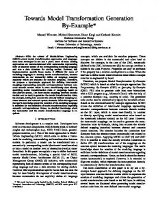
Fig. 11. Results of exM Msource ↔ exM Mtarget (left) and Ecore ↔ M injava (right)
6
Case study
This case study compares the results obtained on various metamodels with the different configurations proposed in Section 3. The parameters of the similarity flooding algorithm used in this case study are: ε = 0.05 and threshold = 0.95. Since many of the real world metamodels are designed to express class models, we chose to use those metamodels as a benchmark. The chosen alignment scenarios are: exM Msource ↔ exM Mtarget , Ecore ↔ M injava, Ecore ↔ Kermeta and Ecore ↔ U M L. Ecore [4] is the meta-metamodel and hence a metamodel. Minjava [8] is a simple metamodel for the Java language, that allows to represent the structure of a Java program. Since Minjava imports the models from Java bytecode, it does not provide a way to describe how the methods of the different classes of a program are structured and thus is very similar to Ecore. Kermeta [9] is an extension of Ecore that allows to give a behavorial description of the operations and derived properties of a class model in addition to the structural description. UML [10] is a multi-purpose software modeling language that deals with class models (including behavioral description), use cases or statecharts. Since the elements from the metamodel used in the matching process are not the same for the different configurations of Section 3, we needed a common denominator between those configurations to compare them. This common denominator is the Ecore aligment model produced by the Ecore alignment encoder described in Section 5. This model only shows mappings between non abstract classes, non derived attributes and references, datatypes and enumerations. Those elements are included in all the different configurations. We compare the Ecore alignment model produced by the alignment encoder to an ideal alignment model designed by an expert (standard transformations such as Ecore to Kermeta have been used to build those ideal models). We evaluate our results with common metrics from the information retrieval field [11]. For each alignment, we f ound mappings #correct f ound mappings compute precision = #correct #total f ound mappings , recall = #total correct mappings 12
0,9
0,9
0,8
0,8
0,7
0,7
0,6
0,6
Minimal Basic Standard Full Flattened Saturated
0,5 0,4 0,3
Minimal Basic Standard Full Flattened Saturated
0,5 0,4 0,3
0,2
0,2
0,1
0,1 0
0 Precision
Recall
Precision
F_score
Recall
F_score
Fig. 12. Results of Ecore ↔ Kermeta (left) and Ecore ↔ U M L (right)
and f score = 2×recall×precision recall+precision . We have precision ∈ [0, 1]. The higher is the precision value, the smaller is the set of wrong mappings. recall ∈ [0, 1]. The higher is the recall value, the smaller is the set of the mappings that have not been found. f score is the harmonic mean of precision and recall. f score ∈ [0, 1]. It can be considered as a global measure of the alignment quality. A high value of f score is obtained when the produced alignment has a good quality. The results of our experiments are shown in Fig. 11 and 12. The results show that the best configuration is generally Saturated. On the other hand, the Minimal configuration gives very bad results. Full and Standard configurations, despite using more information from the metamodels, seem to produce slightly poorer results than the Basic configuration. The metamodels we used to match on Ecore vary in size. Minjava has more or less the same size as Ecore, Kermeta is a little bigger, and UML is very large. We can clearly see from the results that the alignment quality decreases when the size difference between the two matched metamodels is increasing. This is partly caused by the SelectThreshold filter that filters the alignment produced by Similarity Flooding. Results on Ecore ↔ M injava and Ecore ↔ Kermeta show that good quality alignments can be produced by our approach.
7
Related work and conclusion
Related Work Automating the discovery of mappings between schemas, ontologies, documents or (meta)models has been thoroughly investigated [1,2]. In the context of Model-Driven Engineering, several approaches for semi-automatic generation of transformations based on mapping have recently been proposed. In [12], model transformations are generated based on ontological information. The two metamodels are supposed to have a semantics given using a mapping onto 13
a known ontology. Reasonning on the ontology then allows to generate a model transformation, adapting a bootstrap transformation that is whether automatically generated or existing. The transformation is written in the paper in QVT Relational. [13] studies the semi-automatic derivation of graph transformation rules based on manual set-up of prototype mappings between models. In another Model Transformation By-Example approach [14], users define a mapping directly on models in concrete syntax (M1 level), then, using a predefined known mapping between concrete and abstract syntaxes, ATL rules can be generated. Compared to these two approaches that are based on a given mapping (onto a pivot ontology or between examples), we focus on automatically determining the mapping on which is based the transformation generation. In [7], the matching operation focuses on classes, datatypes and enumerations. The proposed class matching algorithm iterates until a fix-point is reached on evaluating if two leaf classes match. Characteristics including attributes, references and relationships (based on closure and composition of inheritance, association, agregation, type-of, etc.) are then used: if the number of matching characteristics is greater than a threshold average, the two classes are considered as similar. The exact computation of characteristic similarity is not much detailed in [7], but it is said that they used name, type and graph matching similarity. For datatypes, the possibility of representing a value of a type (e.g. int) by another type (e.g. float) is used. For enumeration, the numbers of identical litterals are compared. Experiments on partial UML and Java metamodels are shown in [15]. In [16], an architecture is proposed for semi-automating the generation of model transformations. A weaving metamodel describes the kinds of links generated by the matching engine and current transformation patterns. Matching is based on element to element and on structural similarities. Structural similarities computation is inspired by the Similarity Flooding approach. A configuration metamodel is introduced to tune the matching phase. Several case studies are conducted in [16]. Here we go deeper into the encoding of metamodels for applying Similarity Flooding. We detail and compare several configurations on known, available, full metamodels. These configurations are helpful for future case tool constructions. The whole process is detailed enough in order to be reproducible and compared to future metamodel matching approaches. Conclusions and perspectives In this paper, we have presented an approach that produces an alignment between two metamodels in an automated way. This approach is based on the application on metamodels of a well-known schema matching algorithm called Similarity Flooding. Our main contribution is the study on the various ways of encoding a given metamodel into a directed labeled graph that can then be exploited by the Similarity Flooding algorithm. We compared six strategies in a case study in terms of precision and recall of the computed mappings between metamodels. This case study points out that the more intuitive encoding strategy (Minimal) leads to poor results, and that the Saturated strategy is the best-suited in the majority of the cases. The generation of an Ecore alignement model (conforming to an Ecore alignment metamodel) from which model transformation code can easily be derived is our second main 14
contribution. Future work will consist in designing code generators both for imperative and declarative languages. We also currently follow another perspective: we study how the Similarity Flooding algorithm can be tuned to our particular domain (metamodel matching). We are working on the way the initial similarity value of a compatiblity node is computed, and on the way we compute the weights of the arcs in the propagation graph.
References 1. Rahm, E., Bernstein, P.A.: A survey of approaches to automatic schema matching. VLDB J. 10(4) (2001) 334–350 2. Shvaiko, P., Euzenat, J.: A survey of schema-based matching approaches. In: J. Data Semantics IV, Volume 3730 of LNCS. (2005) 146–171 3. Melnik, S., Garcia-Molina, H., Rahm, E.: Similarity flooding: A versatile graph matching algorithm and its application to schema matching. In: ICDE, Volume 2593 of LNCS. (2002) 117–128 4. Budinsky, F., Brodsky, S., Merks, E.: Eclipse Modeling Framework. Pearson Education (2003) 5. Pottinger, R., Bernstein, P.A.: Merging models based on given correspondences. In: VLDB. (2003) 826–873 6. Levenshtein, V.: Binary codes with correction of deletions, insertions and substitution of symbols. Dokl. Akad. Nank. SSSR 163(4) (1965) 845–848 7. Lopes, D., Hammoudi, S., Abdelouahab, Z.: Schema matching in the context of model driven engineering: From theory to practice. In: Advances in Systems, Computing Sciences and Software Eng., Springer Netherlands (2006) 219–227 8. Falleri, J.R.: Minjava. http://code.google.com/p/minjava/ (2008) 9. Triskell: Kermeta. http://www.kermeta.org (2008) 10. Eclipse: UML2 EMF Plugin. http://www.eclipse.org/uml2 (2008) 11. Do, H.H., Melnik, S., Rahm, E.: Comparison of schema matching evaluations. In: Web, Web-Services, and Database Systems, Volume 2593 of LNCS, Springer (2002) 221–237 12. Roser, S., Bauer, B.: An approach to automatically generated model transformations using ontology engineering space. In: Proceedings of Workshop on Semantic Web Enabled Software Engineering (SWESE). (2006) 13. Varr´ o, D.: Model transformation by example. In: Proc. Model Driven Engineering Languages and Systems (MODELS 2006). Volume 4199 of LNCS., Genova, Italy, Springer (2006) 410–424 14. Wimmer, M., Strommer, M., Kargl, H., Kramler, G.: Towards model transformation generation by-example. In: HICSS, IEEE Computer Society (2007) 285 15. Lopes, D., Hammoudi, S., de Souza, J., Bontempo, A.: Metamodel matching: Experiments and comparison. In: ICSEA, IEEE Computer Society (2006) 2 16. Fabro, M.D.D.: Metadata management using model weaving and model transformation. PhD thesis, Universit´e de Nantes (2007)
15