International Journal of Computer Engineering and Information Technology VOL. 8, NO. 10, October 2016, 184–188 Available online at: www.ijceit.org E-ISSN 2412-8856 (Online)
Method of Dynamic Data Distribution in Virtual Memory Resources in Cloud Technologies Alakbarov Rashid1, Pashayev Fahrad2 and Alakbarov Oqtay3 1, 3
Institute of Information Technology of ANAS, Baku, Azerbaijan 2
Institute of Control Systems of ANAS, Baku, Azerbaijan
1
[email protected],
[email protected],
[email protected]
ABSTRACT The article focuses on the dynamic data distribution among memory resources in processing centers. The method of dynamic data distribution among various storage devices is offered by using trigonometric model with the trend of specific changes of user file call frequencies depending on time. The change in the file call frequencies depending on time is formulated as the sum of linear and trigonometric functions. Mean square errors minimization method and Fourier allocation method of discrete time series are used to define model coefficients. Developed model ensures more efficient use of memory resources of data storage system and its usage by users more.
Keywords: Data Processing Center, Cloud Technologies, Storage Capacity, Data Call Frequency, Virtual Resource, Memory Resource, Time Trend, Trigonometric Model.
1. INTRODUCTION Hypervisor is used for the optimal efficient use and allocation of virtual memory resources among users. This system helps to eliminate the shortcomings of traditional SAN (Storage Area Network) technology. Applying hypervisor the new functions are used for the control of virtual memory resources. These new functions include process automation, auto-recovery mechanism in the case of incidents, back-ups, dynamic distribution of memory resources (Thin Provisioning) and automated files distribution by levels (Automated Tiered Storage) and others. Joint use of Thin Provisioning and Automated Tiered Storage technologies has a major impact on increasing the efficiency of controlling and distribution of virtual memory [1]. The use of these technologies enables the efficient use of memory resources in clouds by the users. Dynamic data distribution among the levels of data storage system through the use of Cloud services is one of the topical issues.
2. TECHNOLOGY OF DYNAMIC STORAGE DISTRIBUTION AMONG THE USERS IN DATA PROCESSING CENTERS AND THE PROBLEM STATEMENT At present, a lot of research works are conducted out for an effective use of computing and storage resources of data processing centers with the help of Cloud Computing in the world. Cloud Computing is used for the development of distributed computing systems for the solution on high performance problems basing on the computer network. Cloud Computing enables organizations to use computing and storage resources of data processing centers more efficiently. With the help of this technology, the user data is stored and processed on Cloud Computing servers, at the same time, the results are viewed through browsers. Cloud technology enables data processing centers to widely use clustering and virtualization of computing and storage resources [2, 3]. Cloud Computing enables to scale and use physical resources (e.g. processor, storage and disk space) through the Internet. In this case, the data processing and storage processes are considered as a type of service. The proposed technology allows the data processing center to attract more users providing optimal distribution of available storage and system resources among the users [4]. It is known that SAN technology is widely used in the development of virtual memory resources in data processing centers. Applying traditional SAN technology the allocated resource is at full disposal of the user. In addition, when the user does not take full advantage of the resource, other users cannot benefit from the remained unused resources.
International Journal of Computer Engineering and Information Technology (IJCEIT), Volume 8, Issue 10, October 2016
185
A Rashid et. al
Thin Provisioning in SAN systems allows the user to hold only allocated amount of resources, which is currently being used by the user. The resources are used more efficiently in this way. As the allocated memory resource is full its quota is recovered from reserve resources. Thin Provisioning is widely employed in the virtualization of storage resources, and it ensures the use of storage without wastes. This technique allows the resource allocated for any purpose to capture the storage as much as it is fully utilized. The resource is not backed up unless it is used, and does not fill any hard drive capacity. This technology allows to use the centralized large storage in a planned way. Hence, the resources are allocated only as much as it is used without waste. Commercial side is beneficial for both the user and the cloud provider. Thus, the user simply pays for the actual use of the resource rather than reserved one. And the provider is free from unnecessary expenses such as the purchase of additional equipment, its installation, and deployment. At the same time, it is able to offer the same service for a lower price, which leads to attracting more users to the services [4]. It is known that storage devices in data processing centers are based on memory equipments with variety of properties (Solid State Disks (SSD), magnetic disk devices, etc.). The prices of such storage equipment can be different. Depending on which devices the users’ data stored in, the payment for the resource rent is diverse. If a user uses very little amount of data stored in the data processing center over the year, the use of resources stored in magnetic disk device will be better than SSD. In this case, the expenses will be less. As the SSD costs much, the user, of course, spends more when using these devices. Conducted monitoring shows that, frequently used data stored in the storage system usually occupies 20-30% of the total capacity of the system [6]. Taking this into account, 2030% of the memory devices of hybrid data storage systems is comprised by SSD. Since SSD is rather expensive, the user, of course, pays more when using these devices. It should be noted that data transmission speed of SSD located on the first layer is 25-100 times higher than that on the second layer, and consequently, costs 5-10 times more than that one. Therefore, less used data in the storage system is not advisable to be stored in SSDs. The option of automated files (data) distribution by groups (types of memory devices) is one of the important components of the optimal allocation of resources and providing efficiency of their use. The option enables avoiding peak loading, and grouping the files by their characteristics. This function (Automated Tiered Storage) is enabled through automated multilayer control systems. Offered technology allows using memory resources efficiently. It provides placement of data in various storage layers of the data storage systems depending on their usage frequency [6,7]. With the help of this technology the first layer of data center virtual storage includes high-speed
SSD (Solid State Disks). The next layer uses magnetic disk devices Ataachid serial SCSI (SAS), which runs less than SSD and costs less. The third layer uses lower speed serial ATA (SATA) devices, which costs less than abovementioned devices (Figure 1).
Fig. 1. Data distribution (migration) within virtual memory levels by usage frequency
Taking into account the above mentioned, on which level of cloud based data storage system the data should be deployed remains one of the topical issues. This article analyzes the frequency of the users’ call to the data stored in memory resources and proposes the trigonometric model for the solution of efficient data deployment in data storage system in accordance with the frequency of the users’ calls.
3. PROBLEM STATEMENT Various bodies of literature propose the followings to develop a mathematical algorithm for the resolution of the dynamic distribution of the files among finite number of layers [8]: - M - number of layers; - V – total storage capacity of the layers; - - storage capacity of the m-th layer; - I - number of files; - size of the i-th file; - N - number of observations; - moment of observation of the i-th file; - - current frequency of the calls to the i-th file at the nth moment of observation; - - average frequency of the calls to the i-th file; - current period of the calls to the i-th file at the n-th moment of observation; - - average period of the calls to the i-th file; The sum of the storage capacity of the layers shall be equal to the total storage capacity V: ; (1) It should be noted that, current interval of the calls to the ith file at the n-th moment of observation is calculated as follows: (2)
International Journal of Computer Engineering and Information Technology (IJCEIT), Volume 8, Issue 10, October 2016
186
A Rashid et. al
The relation between the current frequency of the calls to the i-th file at the n-th moment of observation and the current interval is as follows: (3) The files’ attributes and call methods are used to define call frequency to the files [8]. Autoregressive methods such as average, moving average, and weighted average methods are applied for the solution of dynamic distribution of the user's files among storage layers in terms of presented agreements and conditions [8]. Each of these methods has own limitations. If the increasing or decreasing trend of call frequency to the files depending on the time is observed, or if hidden or obvious periodicity is observed, the application of these methods can lead to certain errors. Thus, application of other techniques is also needed. When developing the models based on experimental data conditions are set for their simplicity and adequacy [9]. In some particular cases, the models can be set by applying a combination of different methods using trigonometric functions. The article sets forth solution of developing such models.
4. PROBLEM SOLUTION Some practical experiments show that call frequency to some files varies as in the Figures 2 or 3. The diagrams provide the results of observations carried out each minute per day (1440 min.). Here, N = 1440 and 1 minute. The number of observations in the abscissa axis, and call frequency to selected file in the ordinate axis are presented in these diagrams. The time passed since the beginning of observations can be calculated as . Scaled experimental call frequencies to a file selected in a certain period of time can be denoted as . To scale call frequencies within the range can be written. If S = 10, the frequencies can be scaled within the range Figures 2 and 3.
Fig. 2. Increasing call frequency to the files
as in the
Fig.3. Decreasing call frequency to the files
Visual analysis of these graphs shows that the change in the call frequency to the file can be modeled as follows [10, 11]: f (i) = the + b + Acos ((k π / T) i + φ) (4) let’s show the model as a sum of two components. If and (5) First, let’s separate the component . Obviously, the coefficients k and b can be determined by minimizing the mean square difference [12]. Let's assume that (6) Let’s find k and b, which defines the minimum value of mean square difference, using Table 1 in order to define the coefficients k and b (7) These coefficients are found as a solution to the following system: (8) The coefficients k and b found from the solution of this system set linear sum. is defined for the frequencies in the Figure 2 and is defined for the frequencies in the Figure 3 with the software designed for the problem solution. Therefore, the graphs can be built by separating the linear components. In this case, can be taken. The graphs of the separated components according to Figure 3 are provided in Figure 4.
International Journal of Computer Engineering and Information Technology (IJCEIT), Volume 8, Issue 10, October 2016
187
A Rashid et. al
,
It is known that,〖
If we mark Fig. 4. Condition after separating the linear component
Here to clear the function from the noise and to set a model as a trigonometric function, it can be allocated by Fourier series. As we know that, the values of the function are discrete,we can write as follows [11, 13]: . Here , ,
then
. If we put received results in (9)
Coefficients of the series are assumed as follows:
(11) and if we take into account (11) and (6) in (4), we will obtain the following: . Here if we mark as , , , then .
(12)
It is known that, in practical applications the coefficients in less number are used in order to clean the function from noise and to smooth it. We will use here only coefficients , and . The remaining coefficients equal to zero:
Therefore, we can write as follows: (9) If we take into account the data given in Figure 4:
will be obtained. If we set the graph of the model and the difference between the model and experimental data by calculating the data given in Figure 3 with the model parameters we can obtain (Figure 5). In this way, the graph of the difference between the model and experimental data shows that they are white noise and can be denoted as . , . Thus, the value of call frequency to the files with time trend in the N-th observation moment can be taken the value calculated by the formula (12) (13) It should be noted that, this model, which is based on a combination of linear and trigonometric functions, can be applied when the time dependence trend of call frequencies to the files are observed as a mixture of periodical
International Journal of Computer Engineering and Information Technology (IJCEIT), Volume 8, Issue 10, October 2016
188
A Rashid et. al
dependence. In some particular cases, a combination of parabolic functions and trigonometric functions, or a combination of hyperbolic functions and trigonometric functions can be applied. In these cases, the model parameters can be determined by using the methods given in this article.
developed and used in the article can be used to solve similar problems.
ACKNOWLEDGMENT This work was supported by the Science Development Foundation under the President of the Republic of Azerbaijan – Grant № EİF-2014-9(24)-KETPL-14/02/1
REFERENCES
Fig. 5. The graphs of the model and difference
When solving similar issues of data processing centers some of these models can be used for the determination of the final call frequency to different files. Let’s assume that, dynamic distribution by the layers is solved and the files of numbers are deployed in the layers. The distribution shall provide the following conditions in accordance with initial conditions (1): ; (14) number of the files can be deployed in the m-1 number of layers up to m-th layer. As a result, the followings shall be implemented for the solution of the dynamic distribution of the files among finite number of layers: 1) The call periods and frequencies to the experimental data files at the moments of observation shall be formed; 2) The average frequencies shall be formed out for clustering by applying appropriate model; 3) The average frequencies and appropriate files shall be arranged in increasing order regularly; 4) Clustering and distribution by groups shall be carried out.
5. CONCLUSION The article presents one of the method for the solution of dynamic (automatic) distribution of i number of given files among the layer M. In this case, clustering algorithm and method are given using current values obtained in the moments of observation of file call frequencies, and in particular cases, applying trigonometric model with the trend. To determine model parameters the mean quadratic difference minimization method and Fourier allocation method of discrete time series are used. The algorithms
[1] Christian Marcinek. Hypervisors of data storage systems. http://www.osp.ru/lan/2012/04/13014691. [2] A.M.Alguliev, R.G.Alakbarov. “Cloud Computing: Modern State, Problems and Prospects”. Telecommunications and Radio Engineering. Volume 72, Number 3, USA. 2013, p 255-266. [3] Marios D. Dikaiakos, George Pallis, Dimitrios Katsaros, Pankaj Mehra, Vakali Athena. Cloud Computing, Distributed Internet Computing for IT and Scientific Research // IEEE INTERNET COMPUTING - 2009. № 9. P. 10-13. [4] Rashid G. Alakbarov, Fahrad H. Pashaev, Mammad A. Hashimov.Development of the Model of Dynamic Storage Distribution in Data Processing Centers. // I.J. Information Technology and Computer Science, 2015, 05, pp. 18-24. [5] David Floyer. Thin provisioning. http://wikibon.org/wiki/Thin provisioning [6] Sergey Orlov. storagetiering - right place at the right time.http://www.osp.ru/lan/2013/03/13034585/ [7] Jeremy LeBlanc, Adam Mendoza, Mike McNamara, NetAppAshishYajna; Rishi Manocha. “Maximize Storage Efficiency with NetApp Thin provisioning and Symantec Thin Reclamation”, Symantec September 2010 | WP7111. [8] Rashid Alakbarov, Fahrad Pashayev, Mammad Hashimov. Development of the Method of Dynamic Distribution of Users’ Data in Storage Devices in Cloud Technology. // Advances in Information Sciences and Service Sciences (AISS), Vol. 8, Number 1, January 31, 2016. [9] Aliyev T.I. Fundamentals of system projecting. SPb: ITMO University, 2015. 120 p. [10] James Stewart. Calculusearly transcendentals. Seventh edition, Brooks/Cole 2012,1356 p. [11] Anirudh Kondaveeti. (2015) Forecasting Time Series Data with Multiple Seasonal Periods. https://blog.pivotal.io/data-sciencepivotal/products/forecasting-time-series-data-withmultiple-seasonal-periods [12] Gavrilov V.I., Makarov Y.N., Chirskiy V.G. Mathematical analysis. M.: "Academy". 2013. 336 p. [13] David W. Kammler. A First Course in Fourier Analysis. Cambridge University Press, 2008, 862 p.