Method of Lyapunov Functions for Systems with Higher-order Sliding

c Pleiades Publishing, Ltd., 2011. ISSN 0005-1179, Automation and Remote Control, 2011, Vol. 72, No. 5, pp. 944–963.  c A.E. Polyakov, A.S. Poznyak, 2011, published in Avtomatika i Telemekhanika, 2011, No. 5, pp. 47–68. Original Russian Text 

NONLINEAR SYSTEMS

Method of Lyapunov Functions for Systems with Higher-order Sliding Modes A. E. Polyakov∗ and A. S. Poznyak∗∗ ∗

∗∗

Trapeznikov Institute of Control Sciences, Russian Academy of Sciences, Moscow, Russia The Research and Advanced Studies Center of the National Polytechnic Institute (CINVESTAV), Mexico City, Mexico Received April 18, 2008

Abstract—For the control systems with higher-order sliding modes, a method was proposed to construct the Lyapunov functions on the basis of the method of characteristics for solution of a special first-order partial derivative equation. Its successful solution enables one to generate the Lyapunov function which proves that the convergence time is finite and estimates explicitly the time of reaching the sliding mode. DOI: 10.1134/S0005117911050043

1. INTRODUCTION At the end of the XIX century, A.M. Lyapunov proposed a simple approach to the problem of studying stability of the equilibrium of the system of ordinary differential equations (ODE). Its concept relies on the generalized notion of “energy” enabling one to analyze a system for stability or instability using only the information about the right-hand side and doing without the exact solution. At first, these methods were used only for the ODE’s with the right-hand sides that are continuous in both time and state variables. Later on, some authors [1, 2] studied a wider class of differential equations where the right-hand sides are discontinuous in these variables. Such equations are now considered as differential inclusions. They also include the so-called sliding mode systems which invite attention of the researchers over the last four decades [3–6]. The finite time of reaching the sliding surface is one of the most important distinctions of the sliding mode systems. In this case, the corresponding Lyapunov functions may be nonsmooth. For example, in [2] for the first-order sliding systems the simplest of which is given by x(t) ˙ = −r sgn [x(t)] , ⎧ ⎪ ⎨

sgn[x] :=

r > 0,

1 if x > 0 −1 if x < 0 ⎪ ⎩ ∈ [−1, 1] if x = 0,

(1.1) (1.2)

the Lyapunov function is V (x) = |x|, and in virtue of system (1.1), for x = 0 its complete derivative satisfies V˙ (x(t)) = −r. Whence it follows that 0  V (x(t)) = V (x(0)) − rt and the reach time treach = V (x(0))/r. For the second-order sliding systems (see [3]) such as ˙ x ¨(t) = −r1 sgn[x(t)] − r2 sgn[x(t)], 944

r1 > r2 > 0,

(1.3)

METHOD OF LYAPUNOV FUNCTIONS

945

the proof of convergence in finite time and the estimate of this time were obtained mostly using the methods of differential geometry on plane [3] which nobody was able to generalize to the vector case. Later on, the Lyapunov function V (x, x) ˙ = r1 |x| + x˙ 2 /2,

(1.4)

which can guarantee only the asymptotic stability because V˙ (x(t), x(t)) ˙  0 was established for system (1.3) [7]. The existing methods of studying the higher-order sliding systems are based on the uniformity principle [8–10] according to which the asymptotically stable uniform system converges in a finite time. Within the limits of this approach, however, it is impossible to estimate the time of reaching the sliding mode. Therefore, not a single method was proposed enabling one to prove system convergence in a finite time and estimating this time. The present paper is devoted to extending the method of Lyapunov functions to the higher-order sliding mode systems which enables one to resolve the aforementioned problems. 2. METHOD TO GENERATE THE LYAPUNOV FUNCTIONS WITH FINITE CONVERGENCE TIME 2.1. System Description Let us consider a control system given by 

x˙ = g(x, y) y˙ = a(x, y) + b(x, y)u + f (t, x, y),

(2.1)

where x ∈ Rk and y ∈ Rn are the components of the system state vector, g : Rk × Rn → Rk and a : Rk × Rn → Rn are the smooth vector functions, u ∈ Rm is the vector of control inputs, b : Rk × Rn → Rn×m is the matrix of feedback gains, and f : R+ × Rk × Rn → Rn is an unknown bounded function, that is, |fj (t, x, y)|  Cj

∀x ∈ Rk ,

∀y ∈ Rn ,

∀t  0,

j = 1, n.

(2.2)

It is assumed that the stabilizing control u, which can be discontinuous, u=u ¯(x, y)

(2.3)

has already been constructed and it is required to prove with the use of the method of Lyapunov function that the zero solution (0, 0) of system (2.1) with control (2.3) is stable simply asymptotically or with a finite time of convergence. 2.2. Generalization of the Zubov Method Let V (x, y) be a continuous function and its derivative along the trajectories of system (2.1) almost everywhere can be estimated as u(x, y) + f (t, x, y) V˙ = ∇x V, g(x, y) + ∇y V, a(x, y) + b(x, y)¯ u(x, y) + |∇y V | , C ,  ∇x V, g(x, y) + ∇y V, a(x, y) + b(x, y)¯ where ·, · stands for the scalar product, |∇y V | = (C1 , C2 , . . . , Cn ) . By denoting

     ∂V   ∂V   ∂V  ,  , . . . ,  

∂y1

u(x, y) + γj , hj (x, y, γj ) := aj (x, y) + bj (x, y)¯ AUTOMATION AND REMOTE CONTROL

Vol. 72

No. 5

2011

∂y2

j = 1, n,

∂yn

(2.4)    and C = 

946

POLYAKOV, POZNYAK

inequality (2.4) can be rearranged in the componentwise form as 



k k



∂V ∂V ∂V dV  gi (x, y) + hj x, y, Cj sgn dt ∂xi ∂yj ∂yj i=1 j=1



.

We seek the Lyapunov function V (x, y) as a continuous positive definite solution of a partial derivative equation like k

i=1



∂V where γj = Cj sgn ∂yj

gi (x, y)

k

∂V ∂V + hj (x, y, γj ) = −qV ρ , ∂xi j=1 ∂yj

(2.5)

and q > 0, ρ > 0 are some positive parameters.

Remark 1. If V (x, y) is a suitable solution of Eq. (2.5), then valid is the inequality dV (x(t), y(t))  −qV ρ (x(t), y(t)), dt and in the case of ρ < 1 we obtain the Lyapunov function with a finite time of convergence 1 [V (x(0), y(0))]1−ρ , and for ρ  1 this function guarantees only the asymptotic treach  q(1 − ρ) stability. To solve Eq.

(2.5), one needs to know the sectionally constant functions γj which in turn depend ∂V . Fortunately, since γj can take only two possible values Cj and −Cj , (2.5) may be on sgn ∂yj considered assuming that γj is equal to either of the aforementioned constants. The exact value of γj can be determined only after finding the general form of the function V (x, y). V.I. Zubov was the first to formulate the idea of seeking the Lyapunov function as a solution of a partial derivative equation [11]. The generalization of the Zubov method that was proposed by the present authors makes it possible for the right-hand sides of Eq. (2.5) to be nonlinearly dependent on the desired function V as well. This generalization enables one to determine the Lyapunov functions with a finite time of convergence. 2.3. Method of Characteristics Equation (2.5) with constant γ can be solved using the so-called method of characteristics [12] according to which the following lemma can be formulated. Lemma 1. If an absolutely continuous positive definite function V (x, y) satisfies the ODE system dxk dy1 dyn dV dx1 = ... = = = ... = = g1 (x, y) gk (x, y) h1 (x, y, γ1 ) hn (x, y, γn ) −qV ρ

(2.6)

for x 2 + y 2 > 0, then it is a solution of Eq. (2.5). This and the following statements are proved in the Appendix. We assume that we have succeeded in determining the first integrals of system (2.6) ϕi (V, x, y, γ, q, ρ) = const := ci ,

i = 1, n + k.

AUTOMATION AND REMOTE CONTROL

(2.7) Vol. 72

No. 5

2011

METHOD OF LYAPUNOV FUNCTIONS

947

Since any function of constants also is a constant (in a special case, zero), the function V (x, y, γ, q, ρ) can be determined as a solution of the nonlinear algebraic equation Φ(ϕ1 (V, x, y, γ, q, ρ), . . . , ϕn+k (V, x, y, γ, q, ρ)) = 0,

(2.8)

where Φ(ϕ1 , . . . , ϕn+k ) is an arbitrary function. Any analytical solution of Eq. (2.8) defines a possible candidate for the Lyapunov function. However, the function Φ and the parameters γ, q, ρ must be selected so that the determined function V (x, y) be absolutely continuous and positive definite. Remark 2. Obviously, the proposed method does not offer a formal algorithm for construction of the Lyapunov function and just assists in determining a candidate for the Lyapunov function, thus reducing the problem of determining a suitable “energy” function to the problem of correct determination of the candidate function parameters. The proposed method will be used in what follows to generate Lyapunov functions with finite convergence time (0 < ρ < 1) for the second-order sliding systems. 3. GENERATION OF THE LYAPUNOV FUNCTION FOR THE “TWIST” ALGORITHM 3.1. Description of the System Let us consider a control system given by 

x˙ = y y˙ = f (t, x, y) + u(t),

(3.1)

where x, y ∈ R are the state variables, f (t, x, y) is an unknown bounded function describing the external perturbations and system uncertainties, and u ∈ R is the second-order sliding control u(t) = −r1 sgn[x(t)] − r2 sgn[y(t)],

(3.2)

where r1 , r2 > 0 are the control parameters and the operator sgn[·] has the form of (1.2). This algorithm is known as the “twist” algorithm [13, 14] It is assumed that |f (t, x, y)|  C

∀x, y ∈ R and ∀t  0,

(3.3)

where C is some certain constant. The aim of the present authors is to generate a Lyapunov function proving convergence of the solutions of system (3.3) to the origin (0, 0) in a finite time and estimate this time. 3.2. Determination of the Candidate Function For a continuous function V (x, y), let there be the following estimate of the total derivative calculated along the trajectories of system (3.1) ∂V ∂V dV =y + (u + f (t, x, y)) dt ∂x ∂y    ∂V ∂V ∂V ∂V ∂V + u + C sgn =y − sgn[x]γ :  y ∂x ∂y ∂y ∂x ∂y   ∂V . γ = r1 + r2 sgn[xy] − γ0 , γ0 = C sgn x ∂y AUTOMATION AND REMOTE CONTROL

Vol. 72

No. 5

2011

(3.4)

948

POLYAKOV, POZNYAK

According to the proposed method, we obtain Eq. (2.5) given by y

∂V ∂V − sgn[x]γ = −kV 1/2 , ∂x ∂y

(3.5)

where k > 0 is a positive parameter. Assuming that γ0 is a constant, we determine solution of (3.5). The corresponding system (2.6) of the characteristic equations is given by dy dV dx √ , = = y − sgn[x]γ −k V

(3.6)

and the first integrals are correspondingly y2 , ϕ1 (x, y) = |x| + 2γ

√ y sgn[x] 2 V ϕ2 (V, y) = − . γ k

(3.7)

We select Φ as √ Φ(ϕ1 , ϕ2 ) = k0 ϕ1 + ϕ2 = 0,

(3.8)

where k0 is a real parameter. Substitution of (3.7) in (3.8) provides the equation  √ y sgn[x] y2 2 V = + k0 |x| + . k γ 2γ

(3.9)

Obviously, the right-hand side of Eq. (3.9) makes sense if and only if γ > 0 or, which is the same, if r1 > r2 + C. Additionally, the left-hand side of Eq. (3.9) is always nonnegative. Therefore, 

sgn[xy] 2/γ . k0 > −  1 + 2γ|x|/y 2

(3.10)

Then, the function V (x, y) can be established from (3.9) as ⎛



⎞2

y2 ⎠ k 2 ⎝ y sgn[x] + k0 |x| + . V (x, y) = 4 γ 2γ

(3.11)

3.3. Elimination of Discontinuities One can easily see that function (3.11) generally is discontinuous and the parameters k0 and k must be selected so as to eliminate the discontinuities. Consideration of the limits of the function V (x, y) for x tending to zero for any fixed y and for y tending to zero for any fixed x gives rise to the following expressions: for

k2 x → 0 V (x, y) → 4 for



k0 sgn [xy] +√ γ 2γ 2 2 k k0 |x| . V (x, y) → 4

y→0

2

y2,

Then, to eliminate the discontinuities on the lines x = 0 and y = 0 it suffices to solve the system ⎧  k0 2 ¯2 sgn[xy] ⎪ ⎪ ⎨ k2 +√ =k ⎪ ⎪ ⎩

γ

2γ

k2 k02 = 1 AUTOMATION AND REMOTE CONTROL

Vol. 72

No. 5

2011

METHOD OF LYAPUNOV FUNCTIONS

¯ Whence it follows that for a number k. 

k=



 γ  ¯   2γ k − 1 > 0, 2

k0 =

2 sgn[xy] √ . γ 2γ k¯ − 1

By uniting (3.12) with condition (3.10), we can formulate the following lemma. Lemma 2. If r1 > r2 + C, r2 > C and k¯ satisfies the inequality 1 1  < k¯ <  , 2(r1 + r2 − C) 2(r1 − r2 + C)

949

(3.12)

(3.13)

then k0 > 0 and condition (3.10) is satisfied for all xy = 0. Therefore, the thus-redefined in continuity Lyapunov function (3.11) is as follows: ⎧   2 ⎪ 2 2 ⎪ y k y sgn[x] ⎪ ⎪ ⎪ + k0 |x| + for xy = 0 ⎪ ⎨ 4 γ 2γ

V (x, y) =

⎪ ⎪ ⎪ ⎪ ⎪ ⎪ ⎩

(3.14)

k¯2 y 2 /4

for x = 0

|x|/4

for y = 0,

where k and k0 are calculated from (3.12) and k¯ satisfies (3.13). 3.4. Main Theorem of the “Twist” Algorithm ∂V reverses sign on the curve It is easy to prove that in the general case the partial derivative ∂y  parameters of system (3.1)–(3.3). L |x| sgn [x] + y = 0 where L is a constant depending on the   However, by redefining γ (see (3.4)) as a function of sgn L |x| sgn [x] + y one again has to eliminate the discontinuities of the Lyapunov function. Therefore, the following choice of γ γ := r1 + (r2 − C) sgn [xy]

(3.15)

is preferable despite the fact that it worsens the estimates in the main theorem. Theorem 1. If r1 > r2 + C and r2 > C, then the function V (x, y) of form (3.14) with γ as (4.25) has the following properties: (1) V (x, y) is a continuous positive definite function over the entire space R2 which is continuously differentiable for xy = 0; (2) the total derivative of the function V (x, y) along the trajectories of system (3.1)–(3.3) satisfies the inequality r1 − r2 − C  d V (x(t), y(t))  −kmin V (x(t), y(t)) (3.16) dt r1 − r2 + C almost for all t with kmin

r1 + (r2 − C)δ √ := min(k) = min δ∈{−1,1} 2

   √  1 ¯  k 2 −  ;  r1 + (r2 − C)δ 

(3) the corresponding guaranteed convergence time is estimated as treach 

2 (r1 − r2 + C)  V (x(0), y(0)). kmin (r1 − r2 − C)

(3.17)

Remark 3. For the case where condition (3.3) is satisfied only in some local neighborhood of the original D0 and the domain of initial data D(cmax ) is determined from the relations D(c) = {(x, y) ∈ R2 : V (x, y)  c} and cmax = max c, one can readily prove with the use of the c:D(c)⊆D0

generated Lyapunov function (3.14) that system (3.1)–(3.2) converges locally in a finite time. AUTOMATION AND REMOTE CONTROL

Vol. 72

No. 5

2011

950

POLYAKOV, POZNYAK

3.5. Numerical Example for the “Twist” Algorithm Let system (3.1)–(3.3) have the following parameters: r1 √= 1.3, r2 = 0.7, and C = 0.1. The corresponding Lyapunov function (3.14) is given for k¯ = 0.9/ 2 by ⎧  2  √ 2 2 ⎪ (0.9 γ − 1) 2γ|x| + y ⎪ ⎪ ⎪ |y| + for xy = 0 √ ⎪ ⎪ 8γ 0.9 γ − 1 ⎨

V (x, y) =

⎪ ⎪ ⎪ ⎪ ⎪ ⎪ ⎩

0.10125y 2

for x = 0

0.25|x|

for y = 0,

3

3

2

2

1

1

0

0

y

y

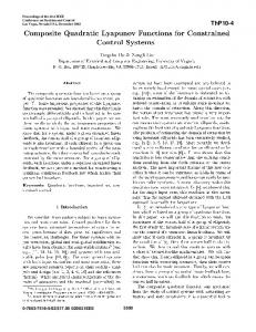
where γ = 1.3 + 0.6 sgn [xy]. Figure 1 depicts the level lines for the given Lyapunov function. Numerical simulation of the transient process (Fig. 2) for f (t, x, y) = C sgn (y) demonstrated convergence of the solution of system (3.1)–(3.3) from the point (1, −2) to the origin in the time est tex reach = 8.72, the estimate by the method of Lyapunov function being treach  15.63.

–1

–1

–2

–2

–3 –2

–1

0 x

1

2

Fig. 1. Level lines of the Lyapunov function for the “twist” controller.

–3 –2

–1

0 x

1

2

Fig. 2. System trajectory with a “twist” controller.

4. CONSTRUCTION OF THE LYAPUNOV FUNCTION FOR THE “SUPER-TWIST” ALGORITHM 4.1. Description of the System We consider the system x˙ = u(t) + ϕ(t),

(4.1)

where x ∈ R is a scalar variable, ϕ(t) is an unknown function describing the indefinitenesses in the model parameters and external perturbations, and u ∈ R is the so-called “super-twist” controller [13, 15]: 

u(t) = u1 (t) + u2 (t), 

u1 (t) = −α |x(t)| sgn [x(t)], u˙ 2 (t) = −β sgn [x(t)],

(4.2) α>0

(4.3)

β > 0,

where α > 0 and β > 0 are the control parameters and the operator sgn [·] is given by (1.2). AUTOMATION AND REMOTE CONTROL

Vol. 72

No. 5

2011

METHOD OF LYAPUNOV FUNCTIONS

951

It is assumed that |ϕ(t)| ˙ L

∀t  0

(4.4)

sgn [x(τ )]dτ,

(4.5)

with a certain constant L. By means of the transformation y(t) = ϕ(t) − β

t 0

the original system (4.1) may be rearranged in 



x(t) ˙ = −α |x(t)| sgn [x(t)] + y(t) y(t) ˙ = ϕ(t) ˙ − β sgn [x(t)],

(4.6)

which is convenient for using the above method of construction of the Lyapunov functions. Now it suffices to construct a Lyapunov function guaranteeing convergence of the solution of system (4.6) to the origin (0, 0) in a finite time in order to prove that in it there exists a second-order sliding mode. 4.2. Finding a Candidate Function Let the continuous function V (x, y) almost everywhere have 



 ∂V ∂V ∂V ∂V dV = x˙ + y˙  −α |x| sgn [x] + y − sgn [x]γ , dt ∂x ∂y ∂x ∂y   ∂V . γ = β − L sgn x ∂y

(4.7)

According to the proposed method, Eq. (2.5) goes over to 





y − α |x| sgn [x]

1 ∂V ∂V − sgn [x]γ = −kV 2 , ∂x ∂y

(4.8)

where k > 0 is a parameter. Assuming that γ is constant, we solve Eq. (4.8). The corresponding system (2.6) of characteristic equations is given by dy dV dx √ . = = −sgn [x]γ −α |x| sgn [x] + y −k V 

(4.9)

Using the change of variables 

z=

|x| sgn [x] , y

the first equation of system (4.9) is reduced to an equation with separable variables −

dy 2γzdz = . − αz + 1 y

2γz 2

(4.10)

Assuming that α2 < 8γ, we determine from (4.10) the first integral of system (4.9): ψ1 (x, y) = AUTOMATION AND REMOTE CONTROL

ln |s(x, y)| + m(x, y), 2 Vol. 72

No. 5

2011

(4.11)

952

POLYAKOV, POZNYAK

where g = 8γ/α2 > 1 and 

s(x, y) = 2γ|x| − α |x| sgn [x]y + y 2 , m(x, y) = √

1 arctan g−1





αg |x| sgn [x] − 2y √ 2 g − 1y

(4.12)



.

(4.13)

The second equation of system (4.9) already is that with separable variables. Then, √ y sgn [x] 2 V − . ψ2 (y, V ) = γ k

(4.14)

We take Φ as Φ(ψ1 , ψ2 ) = k0 eψ1 + ψ2 = 0,

(4.15)

where k0 is a real parameter. By substituting (4.11) and (4.14) in (3.8), we obtain √  y sgn [x] 2 V = + k0 em(x,y) s(x, y), k γ

(4.16)

where s(x, y) and m(x, y) are given by (4.12) and (4.13), respectively. Lemma 3. If g > 1, then s(x, y) > 0 for x2 + y 2 = 0. Equation (3.9) is correct only if for x2 + y 2 = 0 its right-hand side is positive. Whence follows the condition k0 > −

sgn [x]y  . s(x, y)

(4.17)

γem(x,y)

In this case, the candidate for the Lyapunov function V (x, y) is given by k2 V (x, y) = 4



 y sgn [x] + k0 em(x,y) s(x, y) γ

2

,

(4.18)

where s(x, y) and m(x, y) are given by (4.12) and (4.13), respectively. 4.3. Elimination of Discontinuities As in the case of the “twist” algorithm, the next step is elimination of the discontinuities of function (4.18) by special selection of the parameters k and k0 . Consideration of the limits of the function V (x, y) for x tending to zero for any fixed y and y tending to zero for any fixed x provides for

x→0

V (x, y) → for

k2 y2 4

y→0







1 sgn [xy] 1 + k0 exp − √ arctan √ γ g−1 g−1  π sgn [xy] k 2 k02 exp √ γ|x|, V (x, y) → 2 g−1

2

,

and it suffices to solve the system ⎧    2 1 ⎪ 2 sgn [xy] + k exp − √ 1 ⎪ √ ⎪ arctan k = const 0 ⎪ ⎨ γ g−1 g−1 ⎪ ⎪ ⎪ ⎪ ⎩

k 2 k02 exp





π sgn [xy] √ γ = const g−1

AUTOMATION AND REMOTE CONTROL

Vol. 72

No. 5

2011

METHOD OF LYAPUNOV FUNCTIONS

953

in order to eliminate the discontinuities. We obtain     √ ¯√ 1 π sgn [xy]  1 arctan √ k = γ k g − exp − √ − √ , g−1 g−1 2 g−1  

(4.19)



π sgn [xy] sgn [xy] exp − √ 2 g−1   , k0 =  1 π sgn [xy] 1 √ arctan √ γ k¯ g − exp − √ − √ g−1 g−1 2 g−1

(4.20)

where k¯ is a positive number. Lemma 4. If g > 1 and the parameter k¯ satisfies the inequality 







1 π 1 − √ arctan √ exp − √ g−1 g−1 2 g−1 < k¯ √ g   1 π 1 arctan √ + √ exp − √ g−1 g−1 2 g−1 , < √ g

(4.21)

then k0 > 0 and condition (4.17) is satisfied for all xy = 0. Therefore, the Lyapunov function (4.18) redefined in continuity goes over to ⎧ 2 2  k y sgn [x] ⎪ m(x,y) ⎪ ⎪ + k0 s(x, y)e , xy = 0 ⎪ ⎪ γ ⎨ 4

V (x, y) =

⎪ ⎪ ⎪ ⎪ ⎪ ⎩

(4.22)

2k¯2 y 2 /α2 ,

x=0

|x|/2,

y = 0,

where k and k0 are determined from (4.19) and (4.20), k¯ satisfies (4.21), and s(x, y) and m(x, y) are given by (4.12) and (4.13), respectively. 4.4. Main Theorem for the “Super-twist” Algorithm  ∂V  . The following lemma Now it is time to recall that γ is not a constant and depends on sgn ∂y enables one to simplify selection of an appropriate γ. Lemma 5. If the conditions of Lemma 4 are satisfied and 



∂V then sgn ∂y



1 1 exp − √ arctan √ 2 g−1 g−1 k¯ > + √ g g





π − √ 2 g−1



,

(4.23)

= sgn [y] for all xy = 0.

Consequently, it is preferable to take a parameter k¯ satisfying simultaneously conditions (4.21) and (4.23), that is, k¯ must belong to I(g): ⎛















⎞

1 1 π 1 1 π 2 exp − √g−1 arctan √g−1 − 2√g−1 exp − √g−1 arctan √g−1 + 2√g−1 ⎠ , . I(g) = ⎝ + √ √ g g g

(4.24)

For such k, the parameter γ takes on the form γ := β − C sgn [xy]. AUTOMATION AND REMOTE CONTROL

Vol. 72

No. 5

2011

(4.25)

954

POLYAKOV, POZNYAK

Lemma 6. For any fixed g > 1, the interval I(g) is nonempty. On the other hand, g depends on γ ∈ {β + L, β − L}. Whence it follows that k¯ indeed has to belong to the intersection of the intervals I(g− ) and I(g+ ): g− =

8(β − L) , α2

g+ =

8(β + L) . α2

(4.26)

Therefore, we get additional constraints on the parameters α and β: a, β > 0 : I(g − ) ∩ I(g+ ) = 0,

(4.27)

where I(g) is given by (4.24) and g + , g− are determined from (4.26). Theorem 2. If α2 < 8(β − L) and condition (4.27) is satisfied, then the function V (x, y) of the form (4.22) with k, k0 , and γ given by (4.19), (4.20), and (4.25), respectively, k¯ ∈ I(g+ ) ∩ I(g− ) has the following properties: (1) V (x, y) is a continuous positive definite function over the entire space R2 which is continuously differentiable for xy = 0; (2) the total derivative V (x, y) along the trajectories of system (4.6) satisfies the inequality   d V (x(t), y(t))  −k V (x(t), y(t))  −kmin V (x(t), y(t)) dt

(4.28)

almost for all t where kmin := min(k)

    1 π(8β − α2 g)  1 α √  ¯√ √ min arctan √ g k g − exp − √ − = √  ;  g−1 g−1 16L g − 1  8 g∈{g− ,g+ } 

(3) the corresponding convergence time is estimated as treach 

2  V (x(0), y(0)).

kmin

Condition (4.27) defines implicit constraints on the parameters α and β which are not very handy for the design of control. The following lemma gives explicit conditions for the parameters. Lemma 7. If β > 5L and 32L < α2 < 8(β − L), then condition (4.27) is satisfied. Remark 4. Estimate (4.28) of the total derivative of the Lyapunov function is reachable. In (4.28), equality takes place for ϕ(t): ϕ(t) ˙ ≡ L sgn [y(t)]. 4.5. Numerical Example for the “Super-twist” Algorithm Let system (4.6) have the parameters α = 1.8, β = 1, and L = 0.1. In this case we get g− = 2.22 and g + = 2.72 and can take k¯ = 0.9834 ∈ I(g− ) ∩ I(g+ ) = (0.9833; 1.2236). Figure 3 depicts the level lines of the Lyapunov function like (4.22) with the aforementioned parameters. Numerical simulation of the transient process (Fig. 4) for the perturbations given by 

ϕ(t) =

−0.1t,

if

0  t  1.5

0.1t − 0.3,

if

t > 1.5

AUTOMATION AND REMOTE CONTROL

Vol. 72

No. 5

2011

METHOD OF LYAPUNOV FUNCTIONS

Fig. 3. Level lines of the Lyapunov function for the “super-twist” controller.

955

Fig. 4. Trajectory of the system with the “super-twist” controller.

demonstrated convergence of the solution of system (4.6) from the point (1, 0) to the origin in time tex reach = 1.6, whereas the same estimate made if using the method of Lyapunov function is  2.25. test reach 5. CONSTRUCTION OF THE LYAPUNOV FUNCTION FOR THE “NESTED” SECOND-ORDER SLIDING ALGORITHM 5.1. Description of the System Let us consider system (3.1), (3.3) with “nested” second-order sliding mode controller (see [13]) 

u(t) = −α sgn [y(t) + β |x(t)| sgn (x(t))],

(5.1)

where α, β > 0 are the control parameters and the operator sgn [·] is given by (1.2). In a system with a control of the given type, solution may converge to the origin in two ways [13]. 2 For 2(α − C) > β , on the curve y + β |x| sgn [x] = 0 along which the solution hits the origin in a finite time there arises a first-order sliding mode. For 2(α + C) < β 2 and under some additional assumptions, the solution “twists” to the origin in a finite time. The first case needs no sophisticated constructions [13] because one has to prove only occurrence of the first-order sliding mode and the convergence time finiteness follows from the first equation of system (3.1) and the condition  y + β |x| sgn [x] = 0. Therefore, we consider only the second case. 5.2. Finding Candidate Function Let us almost everywhere have for the continuous function V (x, y) 



 ∂V  ∂V ∂V ∂V dV  + u(t) ∂V = y ∂V − sgn [z]γ ∂V , =y + (u(t) + f (t, x, y)) y + C  dt ∂x ∂y ∂x ∂y  ∂y ∂x ∂y   ∂V , (5.2) γ = α − C sgn z ∂y 

z = z(x, y) := y + β |x| sgn (x).

(5.3)

In compliance with the proposed method, we obtain Eq. (2.5) in terms of y

∂V ∂V − sgn [z]γ = −kV 1/2 , ∂x ∂y

AUTOMATION AND REMOTE CONTROL

Vol. 72

No. 5

2011

(5.4)

956

POLYAKOV, POZNYAK

where k > 0 is a parameter. The corresponding system (2.6) of characteristic equations is given by dx dy dV √ , = = y −sgn [z]γ −k V

(5.5)

and the first integrals, respectively, by √ y sgn [z] 2 V ϕ2 (V, y) = − . γ k

y2 ϕ1 (x, y) = x sgn [z] + , 2γ

(5.6)

We take Φ in terms of √ Φ(ϕ1 , ϕ2 ) = k0 ϕ1 + ϕ2 = 0,

(5.7)

where k0 is a real parameter. Substitution of (5.6) in (5.7) provides the equation  √ y sgn [z] y2 2 V = + k0 x sgn [z] + . k γ 2γ

(5.8)

Lemma 8. If γ > 0 and β 2 > 2γ, then x sgn [z] + y 2 /(2γ) > 0 for x2 + y 2 = 0. Since the right-hand side of (5.8) must be positive for x2 + y 2 = 0, 

2/γ sgn [yz] . k0 > −  1 + 2γ|x| sgn [xz]/y 2

(5.9)

In this case, the function V (x, y) goes over to ⎛

⎞2



y2 ⎠ k 2 ⎝ y sgn [z] + k0 x sgn [z] + . V (x, y) = 4 γ 2γ

(5.10)

5.3. Elimination of Discontinuities Now one has to eliminate the discontinuities of function (5.10) on the straight line x = 0 and  the curve z = y + β |x| sgn [x] = 0: x→0

for for





V (x, y) → k2 y 2 1/γ + k0 / 2γ 

2

/4,



z → 0 V (x, y) → k 2 |x| −β sgn [xz]/γ + k0 β 2 /(2γ) + sgn [xz]

2

/ 4.

Whence it follows that k0 and k must satisfy the equation system 



k 2 1/γ + k0 / 2γ

2



= 1 and



k2 k0 β 2 /(2γ) + sgn [xz] − β sgn [xz]/γ

2

= k¯2

¯ Then, we obtain for xz = 0 that for some positive k. 

k0 =

k¯ + β sgn [xz] 2  γ β 2 + 2γ sgn [xz] − k¯

√ and

2γ

. k =    2/γ + k0 

(5.11)

√ Lemma 9. If 0 < γ < β 2 /2 < 2γ/ 3 and 

β 2 − 2γ < k¯ < β,

(5.12)

then k0 > 0 and condition (5.9) is satisfied for all x2 + y 2 = 0. AUTOMATION AND REMOTE CONTROL

Vol. 72

No. 5

2011

METHOD OF LYAPUNOV FUNCTIONS

957

Therefore, the continuous Lyapunov function (5.10) is as follows:

V (x, y) =

⎧   2 ⎪ ⎪ y2 k2 y sgn [z] ⎪ ⎪ + k0 x sgn [z] + for ⎪ ⎨ 4 γ 2γ ⎪ ⎪ ⎪ ⎪ ⎪ ⎩

xz = 0

y 2 /4

for

x=0

k¯2 |x|/4

for

z = 0,

(5.13)

where k and k0 are determined from (5.11) and k¯ satisfies inequality (5.12). 5.4. Main Theorem for the “Nested” Algorithm By taking γ := α − C,

(5.14)

one may formulate the following theorem. √ √ √ Theorem 3. If α > C(2 + 3)/(2 − 3) and 2(α + C) < β 2 < (α − C)4/ 3, then the function V (x, y) like (5.13) with γ defined in (5.14) has the following properties: (1) V (x, y) is a continuous positive definite function in the space R2 which is continuously differentiable for all xz = 0; (2) the total derivative of the function V (x, y) along the trajectories of system (3.1), (3.3), (5.1) satisfies the inequality   d V (x(t), y(t))  −qk V (x(t), y(t))  −qkmin V (x(t), y(t)) dt √ ¯ γ| β 2 +2γδ−k| ; almost for all t, where q = 1 − 6C/γ and kmin := min(k) = minδ∈{−1,1} √ 2

(3) the convergence time is estimated as treach 

2 qkmin



|

(5.15)

β +2γδ+βδ|

V (x(0), y(0)).

5.5. Numerical Example for the “Nested” Controller

3

3

0

0

–3

y

y

Let α = 2.8, β = 2.5, and C = 0.2. Then, one may take k = 1.4983. The level lines of the function V (x, y) like (5.13) with the aforementioned parameters are depicted in Fig. 5. Numerical

0 x

3

Fig. 5. Level lines of the Lyapunov function for the “nested” controller. AUTOMATION AND REMOTE CONTROL

Vol. 72

–3

0 x

3

Fig. 6. Trajectory of the system with “nested” controller. No. 5

2011

958

POLYAKOV, POZNYAK

simulation of the transient process (Fig. 6) for f (t, x, y) = −C proved convergence of the solution of system (3.1), (3.3), (5.1) from the point (3, −1) to the origin in time tex reach = 2.72; the estimate  5.45. by the method of Lyapunov function being test reach 6. CONCLUSIONS A method to construct the Lyapunov functions for analysis of finite convergence in the systems with sliding modes of higher orders was proposed. It relies on the method of characteristics for solution of the special partial derivative equation. Despite the fact that the proposed approach gives no formal algorithm to construct the Lyapunov function, it enables one to reduce the problem to correct selection of the parameters guaranteeing absolute continuity and positive definiteness of the desired “energy” function. The proposed method was illustrated by the example of three well-known second-order sliding algorithms. APPENDIX Proof of Lemma 1. For x 2 + y 2 > 0, we get V (x, y) > 0 and dV dV dxi = −gi (x, y) ρ , dyj = −hj (x, y, γi ) ρ . qV qV Then, (2.5) follows obviously from dV =

k

∂V i=1

∂xi

dxi +

n

∂V j=1

∂yj

⎡ ⎤ k n



∂V ∂V dV dyj = − ⎣ gi (x, y) + hj (x, y, γi )⎦ , ρ i=1

∂xi

j=1

∂yj

qV

Proof of Lemma 2. %√ &−1 2γ+ k¯ − 1 > (1) We consider the case of xy > 0. Then, one has to verify the inequality % & ∂V −1/2 with γ+ = r1 + r1 + C sgn x which follows directly from the chain of − 1 + 2γ+ |x|/y 2 ∂y inequalities k¯ > (2(r1 + r2 − C))−1/2  (2γ+ )−1/2 . % √ ¯&−1 > (2) For xy < 0, it is necessary to demonstrate that   valid is the inequality 1 − 2γ− k % &−1/2 ∂V 1 + 2γ− |x|/y 2 with γ− = r1 − r1 + C sgn x which follows from the inequality 0 < k¯ < ∂y (2(r1 − r2 + C))−1/2  (2γ− )−1/2 . √ √ √ (3) Since 2γ+ k¯ − 1 > 0 and 2γ− k¯ − 1 < 0, we have sgn [xy] = sgn [ 2γ k¯ − 1] and k0 > 0 for all xy = 0. Proof of Theorem 1. (1) Obviously, the function V (x, y) may have discontinuities only on the straight lines x = 0 and y = 0. The parameters k and k0 (4.19) are selected so as eliminate the discontinuities on them. Consequently, the function V (x, y) is continuous by construction. (2) The partial derivatives of the function V (x, y) are given by k2 ∂V = ∂x 2 k2 ∂V = ∂y 2





k 2 sgn [x] 1 k  √0 + 0 2 1 + 2γ |x| /y 2 2γ



, 

k0 y 2 k0 sgn [x](y 2 + γ|x|) y + 2 + . γ2 2γ γ |x| + y 2 /(2γ)

∂V ∂V and are continuous for x = 0 ∂x ∂y and y = 0. Moreover, in any bounded domain the right and left limits of the partial derivatives are finite on these lines.

Since γ, k, and k0 switch only on the lines x = 0 and y = 0,

AUTOMATION AND REMOTE CONTROL

Vol. 72

No. 5

2011

METHOD OF LYAPUNOV FUNCTIONS

959

(3) We consider the total derivative of the function V (x, y) along the trajectories of system (3.1): √ dV =k V dt





γ¯ − + γ

γ k0 sgn [xy]  2 1 + 2γ|x|/y 2



γ¯ 1− γ



,

where γ¯ = r1 + r2 sgn [xy] − f (t, x, y) sgn [x], γ = r1 + r2 sgn [xy] − C sgn [xy] (see (4.25)). Since γ¯ γ¯ 1  for xy > 0 and 1   (r1 − r2 − C)/(r1 − r2 + C) for xy < 0, the inequality γ γ γ¯ − + γ



γ k0 sgn [xy]  2 1 + 2γ|x|/y 2





γ¯ 1− γ

−

r1 − r2 − C r1 − r2 + C

r1 − r2 − C √ dV  −kmin V for xy = 0. dt r1 − r2 + C (4) It remains to complete the proof by noticing that system (3.1)–(3.3) has no nontrivial solution with x(t) ≡ 0 or y(t) ≡ 0. Stated differently, the system trajectories intersect the switching lines avoiding to move along them [7]. Therefore, inequality (3.16) is satisfied almost everywhere along the trajectories of system (3.1)–(3.3). Proof of Lemma 3. To prove validity of the relation

is satisfied. Therefore, we obtained



2

|x| sgn [x]

s(x, y) = 2γ

−α





|x| sgn [x] y + y 2 > 0 for

x2 + y 2 = 0,

one may use the Sylvester criterion for the quadratic forms. It follows from the condition g = 8γ/α2 > 1 that the corresponding quadratic matrix has positive successive principal minors. Proof of Lemma 4. (1) For xy > 0, we get 

√ k0 = γ −1 k¯ g exp









1 π 1 √ arctan √ − exp − √ 2 g−1 g−1 g−1 

−1





and it follows from (4.21) that k0 > 0 > −y sgn [x]/ γem(x,y) s(x, y) . (2) In the case of xy < 0, one has to prove that 





1 1 arctan √ g−1 g−1 Let us consider the scalar function k0 = γ −1 exp − √

f (p) = e

√ 1 arctan g−1

whose derivative for p  0 is given by f  (p) = −2γpe Since,



f



√1 arctan g−1







√ − √π − k¯ ge 2 g−1

αg 1 √ p+ √g−1 2 g−1

αg 1 √ p+ √g−1 2 g−1

m(x,y)

|x|/ |y| /γ = |y| / γe

we obtain from (4.21) that









−1









3/2

/ 2γp2 + αp + 1

s(x, y)  f (0)/γ = e





/ 2γp2 + αp + 1,



1 1 arctan √ k0 > γ −1 exp √ g−1 g−1



> |y| / γem(x,y) s(x, y) .





 0.

√ 1 arctan g−1





√1 g−1



/γ,



 |y| / γem(x,y) s(x, y) .

Proof of Lemma 5. Under the conditions of Lemma 4, the partial derivative of the function V (x, y) with respect to y is given by   √  ∂V m(x,y) = k V sgn [x]/γ + k0 (y − α |x| sgn [x])e / s(x, y) ∂y AUTOMATION AND REMOTE CONTROL

Vol. 72

No. 5

2011

960



POLYAKOV, POZNYAK   m(x,y)

and one needs to prove that sgn 1 + γk0 (y sgn [x] − α |x|)e



/ s(x, y) = sgn [xy].

(1) Let us consider the function 



1 1 αg arctan √ p−1 − √ f1 (p) = (p − α) exp √ g−1 2 g−1 g−1



/ 2γ − αp + p2 ,

with the following derivative for p  0 f1 (p)



= 2γ exp √



1 1 αg arctan √ p−1 − √ g−1 2 g−1 g−1







/ 2γ − αp + p2



Then, f1 (|y| / |x|) = (|y| − α |x|)em(x,y) / s(x, y)  f1 (0) = −2 exp 

from (4.20), (4.23) that 1 + γk0 (|y| − α (2) For the function 





|x|)em(x,y) /

√π 2 g−1

3/2

> 0.

 √

/ g, and it follows

s(x, y) > 0 for xy > 0.



1 1 αg arctan √ p−1 + √ f2 (p) = (p + α) exp − √ g−1 2 g−1 g−1



/ 2γ + αp + p2

we obtain that for p  0 f2 (p)





1 1 αg arctan √ p−1 + √ = 2γ exp − √ g−1 2 g−1 g−1



/ 2γ + αp + p2

3/2

> 0.

  √    Then, f2 (|y| / |x|) = (|y| + α |x|)em(x,y) / s(x, y)  f2 (0) = 2 exp − 2√πg−1 / g, and we obtain 



from (4.20), (4.21), (4.23) that 1 − γk0 (|y| + α |x|)em(x,y) / s(x, y) < 0 for xy < 0. Proof of Lemma 6. (1) We first prove that 

f1 (x) = exp − √

x 2x + 1





π x + arctan √ 2 2x + 1



+ x/(x + 1) < 1

 √  √ for all x ∈ (0, +∞), that is, ln(1 + x) 2x + 1/x < π/2 + arctan x/ 2x + 1 :  √  √  √ (a) we get for x  1 that ln(1 + x) 2 + 1/x/ x  3 < π/2 + arctan x/ 2x + 1 ; here, the √ inequality 1 + x < exp ( x) is used for x  1;  √  √ (b) we get for 0 < x < 1 that ln(1 + x) 2x + 1/x < π/2 < π/2 + arctan x/ 2x + 1 from  x π √ . 1 + x < exp 2 2x + 1  (2) Now, we consider the function f2 (y) = exp (y (π/2 − arctan (y)))−y/ 1 + y 2 and prove that f2 (y) > 1 for all y ∈ (0, +∞), that is,

π/2 > arctan (y) + y

−1







ln 1 + y/ 1 +

y2

.

Using the L’Hospital rule, we readily obtain that 

arctan (y) + y

lim

y→+0



lim

y→+∞

−1





ln 1 + y/ 1 + 





y2

arctan (y) + y −1 ln 1 + y/ 1 + y 2

= 1,



= π/2.

AUTOMATION AND REMOTE CONTROL

Vol. 72

No. 5

2011

METHOD OF LYAPUNOV FUNCTIONS

961

Therefore, it suffices to verify for strict monotonicity the expression under the sign of limit for y > 0. It follows from the inequality 

arctan (y) + y = 1/(y 2 + 1) + y −1 

−1



ln 1 + y/ 1 +



−1





y2 + 1 + y



y2

 



(y 2 + 1)−1 − y −2 ln 1 + y/ 1 + y 2 



= y/ y 2 + 1 − ln 1 + y/ 1 + y 2



/y 2 > 0.

(3) It was proved that f1 (x) < 1 < f2 (y) for all x, y > 0. Then, for g > 1 we get    % √ & 1 1 −π/2 − arctan 1/ g − 1 √ = √ + exp , f1 √ g−1 g g−1  % √ &  1 1 π/2 − arctan 1/ g − 1 √ = exp −√ , f2 √ g−1 g−1 g whence it follows that the interval I(g) is nonempty. Proof of Theorem 2. (1) The function V (x, y) was constructed using Lemmas 3–6 and special selection of the param¯ It is positive definite and continuous over the entire space R2 . eters k, k0 , and k. (2) The partial derivatives V (x, y) for xy = 0 are given by k2 ∂V = ∂x 2 k2 ∂V = ∂y 2







  y sgn [x] m(x,y) m(x,y) + k0 e s(x, y) k0 γ sgn [x]e / s(x, y), γ

 y sgn [x] + k0 em(x,y) s(x, y) γ





sgn [x] k0 (y − α |x| sgn [x])em(x,y)  + γ s(x, y)



.

∂V ∂V and are continuous ∂x ∂y for all xy =  0. and the right limits of the partial derivatives on these lines are finite in any bounded domain. (3) We consider the total derivative of V (x, y) along the trajectories of system (4.6)

Since γ, k, and k0 switch only on the straight lines x = 0 and y = 0,

∂V ∂V ∂V dV = x˙ + y˙ = dt ∂x ∂y ∂x







y − α |x| sgn [x] +

∂V (ϕ˙ − β sgn [x]) . ∂y

It follows from Lemma 5 and the condition for the parameter k¯ that 







 ∂V  ∂V ∂V ∂V ∂V  |ϕ| ϕ˙   sgn sgn [y]L ˙  L=  ∂y ∂y ∂y ∂y ∂y

and

√ dV  −k V . dt

We notice that k > 0 depends on sgn[xy] and assumes various values for xy > 0 and xy < 0. Therefore, the number kmin = min{k} > 0 may be used to advantage to estimate the convergence time. (4) Finally, to complete the proof, it suffices to notice that the trajectories of system (4.6) intersect the switching lines x = 0 and y = 0 avoiding to move along them. To prove this fact, it suffices to assume the opposite. Consequently, inequality (4.28) is satisfied almost everywhere along the trajectories of system (4.6). Proof of Lemma 7. (1) We first notice that g − < g+ and it follows from β > 5L and 32L < α2 that g+ 1, the functions 1 − √g−1

f1 (g) = 2/g + e



π +arctan 2



√1 g−1



√ / g

and f2 (g) = e

√1 g−1



π −arctan 2



√1 g−1



√ / g

are monotone decreasing because 

f1 (g) =

exp − √ 





⎛ π





⎛

1 π 1 + arctan √ g−1 2 g−1 2

1 π 1 exp √ − arctan √ g−1 2 g−1 f2 (g) = 2





⎞ 1 √ + arctan ⎜2 2−g ⎟ g−1 ⎜ ⎟ − 2 < 0, + √ ⎝ 3/2 3/2 g (g − 1)⎠ g2 g (g − 1) 



⎞ π 1 √ − arctan ⎜ 2 2−g ⎟ g−1 ⎜− ⎟ < 0. + 3/2 √ ⎝ ⎠ 3/2 g (g − 1) g (g − 1)

I(g− ) ∩ I(g+ ) = ∅ only if f1 (g− ) < f2 (g− + 0.25) < (3) Obviously, I(g) = (f1 (g), f2 (g)). Therefore,  g− (f1 (g− ) − 1/g− ) < 1. Finally, the inequality f2 (g+ ). It was proved in Lemma 6 that − − − g (f2 (g + 0.25) − 1/g ) > 1 completes the proof. Proof of Lemma 8. (1) sgn [xz] = sgn [yz] = 1 is satisfied for xy > 0. Consequently, x sgn [z] + y 2 /(2γ) > 0.  (2) For xy < 0, we get sgn [xz] = −sgn [yz] = sgn [β |x| − |y|] :  (a) for β |x| − |y| < 0, we obtain x sgn [z] + y 2 /(2γ)  |x|(β 2 /(2γ) − 1) > 0;  (b) for β |x| − |y| > 0, we obtain x sgn [z] + y 2 /(2γ) = |x| + y 2 /(2γ) > 0.  (3) If y = 0, then x sgn [z] + y 2 /(2γ) = x sgn [β |x| sgn (x)] = |x|  0. Proof of Lemma 9. (1) For xy > 0, inequality (5.9) follows from sgn [yz] = sgn [xz] = 1. (2) For xy < 0, we obtain sgn [xz] = −sgn [yz]: (a) for xz < 0, inequality (5.9) follows from k0 > 0;    ¯ 2/γ(β + k) 2/γ 2/γ sgn [xz] >  . (b) for xz > 0, we have k0 =  2 2 ¯ 1 + 2γ/β 1 + 2γ|x| sgn [xz]/y 2 β + 2γ − k (3) For y = 0, x = 0, we obtain sgn [xz] = 1 and the right-hand side of (5.9) is zero. Proof of Theorem 3. (1) The function V (x, y) is continuous by construction in virtue of a special selection of the parameters k and k0 . (2) The partial derivatives of V (x, y) are as follows: k2 ∂V = ∂x 2 k2 ∂V = ∂y 2

 

k02 sgn [z] k0 y  + 2 2γ x sgn [z] + y 2 /(2γ) k0 (y 2 sgn [z] + γx) k02 y y  + + γ2 2γ γ 2 x sgn [z] + y 2 /(2γ)



, 

.

Their continuity for xz = 0 follows, obviously, from the form of the parameters k and k0 . (3) In virtue of system (3.1), the total derivative of the function V (x, y) has the following estimate: √ dV k V dt





k0 |y| sgn [yz] γ¯ γ¯ − +  2 1− γ 2 y /(2γ) + |x| sgn [xz] γ



AUTOMATION AND REMOTE CONTROL

, Vol. 72

No. 5

2011



where γ¯ = α − C sgn z



METHOD OF LYAPUNOV FUNCTIONS

963

∂V γ¯ , γ = α − C (see (4.25)). Since 1  is valid for all x, y, for yz > 0 we ∂y γ

have the inequality γ¯ − + γ





k0 sgn [yz] γ γ¯  1− 2 2 1 + 2γ|x|/y sgn [xz] γ



 −q.

(A.1)



 γ k0 / 1 + 2γ/β 2 < 4. Consequently, (A.1) is valid in 2 √ dV  −k V for xz = 0. this case as well. Therefore, we obtain dt (4) The proof is completed by noticing that under the condition 2(α + C) < β 2 the trajectories of system (3.1), (5.1) cross the switching lines x = 0 and z = 0 and avoid to move along them. It suffices to assume the opposite to prove this fact, see [13]. Consequently, inequality (5.15) is satisfied almost everywhere along the trajectories of system (3.1), (5.1).

For yz < 0 we get sgn [xz] = 1 and 0 

REFERENCES 1. Filippov, A.F., Differentsial’nye uravneniya s razryvnoi pravoi chast’yu (Differential Equations with Discontinuous Right-hand Side), Moscow: Nauka, 1985. 2. Utkin, V.I., Skol’zyashchie rezhimy v zadachakh optimizatsii i upravleniya, Moscow: Nauka, 1981. Translated into English under the title Sliding Modes in Control Optimization, Heidelberg: Springer, 1992. 3. Levant, A., Sliding Order and Sliding Accuracy in Sliding Mode Control, Int. J. Control, 1993, vol. 58, no. 6, pp. 1247–1263. 4. Edwards, C. and Spurgeon, S., Sliding Mode Control: Theory and Applications, London: Taylor & Francis, 1998. 5. Utkin, V.I., Guldner, J., and Shi, J., Sliding Modes in Electromechanical Systems, London: Taylor & Francis, 1999. 6. Emel’yanov, S.V., Korovin, S.K., and Levantovskii, L.V., New Class of Second-order Sliding Algorithms, Vychisl. Algorit. Metody, 1990, vol. 2, no. 3, pp. 89–100. 7. Orlov, Y., Extended Invariance Principle and Other Analysis Tools for Variable Structure Systems, in Advances in Variable Structure and Sliding Mode Control, Edwards, C., Colet, E.F., and Fridman, L., Eds., Berlin: Springer, 2006, pp. 3–22. 8. Bacciotti, A. and Rosier, L., Liapunov Functions and Stability in Control Theory, in Lecture Notes in Control and Information Sciences, vol. 267, New York: Springer, 2001. 9. Orlov, Y., Finite Time Stability and Robust Control Synthesis of Uncertain Switched Systems, SIAM J. Control Optim., 2005, vol. 43, no. 4, pp. 1253–1271. 10. Shtessel, Y.B., Shkolnikov, I.A., and Levant, A., Smooth Second-Order Sliding Modes: Missile Guidance Application, Automatica, 2007, vol. 43, no. 8, pp. 1470–1476. 11. Zubov, V.I., Ustoichivost’ dvizheniya (metody Lyapunova i ikh primenenie) (Motion Stability (Lyapunov Methods and Their Application)), Moscow: Vysshaya Shkola, 1984. 12. El’sgol’ts, L.E., Differentsial’nye uravneniya i variatsionnoe ischislenie (Differential Equations and Variational Calculus), Moscow: Nauka, 1965. 13. Levant, A., Principles of 2-sliding Mode Design, Automatica, 2007, vol. 43, no. 4, pp. 576–586. 14. Polyakov, A. and Poznyak, A., Lyapunov Function Design for Finite-Time Convergence Analysis: “Twisting” Controller for Second Order Sliding Mode Realization, Automatica, 2009, vol. 45, pp. 444–448. 15. Polyakov, A. and Poznyak, A., Reaching Time Estimation for “Super-Twisting” Second Order Sliding Mode Controller via Lyapunov Function Designing, IEEE Trans. Automatic Control, 2009, vol. 54, no. 8, pp. 1951–1955.

This paper was recommended for publication by B.T. Polyak, a member of the Editorial Board AUTOMATION AND REMOTE CONTROL

Vol. 72

No. 5

2011