Jayshree Sarma, Adrian Grajdeanu, Liviu Panait and Eric âSiggyâ Scott. And finally, ... 3.3.3 The Multivariate Form of the Variance Equation . . . . . . . . 30. 3.3.4 Two ..... 5.30 Scatter plot show parent/offspring trait relationship for an EA using ...... y. For example, if x and y are identical, the resulting covariance matrix will be the.
METHODS FOR IMPROVING THE DESIGN AND PERFORMANCE OF EVOLUTIONARY ALGORITHMS by Jeffrey K. Bassett A Dissertation Submitted to the Graduate Faculty of George Mason University In Partial fulfillment of The Requirements for the Degree of Doctor of Philosophy Computer Science
Committee: Dr. Kenneth A. De Jong, Dissertation Director Dr. Sean Luke, Committee Member Dr. John J. Grefenstette, Committee Member Dr. Pearl Wang, Committee Member Dr. Sanjeev Setia, Department Chair Dr. Kenneth S. Ball, Dean, The Volgenau School of Engineering Date:
Fall 2012 George Mason University Fairfax, VA
Methods for Improving the Design and Performance of Evolutionary Algorithms A dissertation submitted in partial fulfillment of the requirements for the degree of Doctor of Philosophy at George Mason University
By
Jeffrey K. Bassett Masters of Science George Mason University, 2003 Bachelor of Science Rensselaer Polytechnic Institute, 1987
Director: Dr. Kenneth A. De Jong, Professor Department of Computer Science
Fall 2012 George Mason University Fairfax, VA
Copyright © 2012 by Jeffrey K. Bassett All Rights Reserved
ii
Dedication
I dedicate this dissertation to my loving and patient wife Hideko.
iii
Acknowledgments
I would like to thank the following people who made this possible. My advisor Dr. De Jong, who’s guidance throughout this process was invaluable. All of the members of the Evolutionary Computation Laboratory, especially Paul Wiegand, Mark Coletti, Jayshree Sarma, Adrian Grajdeanu, Liviu Panait and Eric “Siggy” Scott. And finally, my committee members, Dr. Sean Luke, Dr. John Grefenstette and Dr. Pearl Wang, all of whom had good advice to offer me along the way.
iv
Table of Contents Page List of Tables . . . . . . . . . . . . . . . . . . . . . . . . . . . . . . . . . . . . List of Figures . . . . . . . . . . . . . . . . . . . . . . . . . . . . . . . . . . . .
viii ix
Abstract . . . . . . . . . . . . . . . . . . . . . . . . . . . . . . . . . . . . . . . 1 Introduction . . . . . . . . . . . . . . . . . . . . . . . . . . . . . . . . . . 2 Background . . . . . . . . . . . . . . . . . . . . . . . . . . . . . . . . . . .
xv 1 8
3
4
2.1
Quantitative Genetics . . . . . . . . . . . . . . . . . . . . . . . . . . .
8
2.2
Evolvability . . . . . . . . . . . . . . . . . . . . . . . . . . . . . . . .
11
2.3
Estimation of Distribution Algorithms . . . . . . . . . . . . . . . . .
13
2.4
Evolutionary Computation Theory . . . . . . . . . . . . . . . . . . .
13
Quantitative Genetics Theory for Evolutionary Algorithms . . . . . . . . .
17
3.1
Price’s Theorem . . . . . . . . . . . . . . . . . . . . . . . . . . . . . . 3.1.1 Sexual Reproduction . . . . . . . . . . . . . . . . . . . . . . .
17 19
3.1.2
Mixing Sexual and Asexual Reproduction
. . . . . . . . . . .
20
3.1.3
The Importance of Variance . . . . . . . . . . . . . . . . . . .
22
3.2
A Re-derivation of the Variance Equation . . . . . . . . . . . . . . . .
23
3.3
Multivariate Phenotypic Traits
. . . . . . . . . . . . . . . . . . . . .
26
3.3.1 3.3.2 3.3.3
Multivariate Normal Distributions . . . . . . . . . . . . . . . . Covariance Matrices . . . . . . . . . . . . . . . . . . . . . . . The Multivariate Form of the Variance Equation . . . . . . . .
26 29 30
3.3.4
Two Forms of Heritability . . . . . . . . . . . . . . . . . . . .
31
Analysis Methods Based on Quantitative Genetics . . . . . . . . . . . . .
33
4.1
Quantifying the Search Space . . . . . . . . . . . . . . . . . . . . . .
33
4.2
4.1.1 Issues . . . . . . . . . . . . . . . . . . . . . . . . . . . . . . . Computational Issues with Matrices . . . . . . . . . . . . . . . . . . .
35 38
4.3
Matrix Similarity Metrics
. . . . . . . . . . . . . . . . . . . . . . . .
40
The Trace Function . . . . . . . . . . . . . . . . . . . . . . . . Similarity Metrics . . . . . . . . . . . . . . . . . . . . . . . . .
41 42
4.3.1 4.3.2
v
5
4.4
Plots . . . . . . . . . . . . . . . . . . . . . . . . . . . . . . . . . . . . 4.4.1 Matrix Ellipse Plots . . . . . . . . . . . . . . . . . . . . . . .
43 43
4.5
Eigenvalue plots . . . . . . . . . . . . . . . . . . . . . . . . . . . . . .
45
Function Optimization . . . . . . . . . . . . . . . . . . . . . . . . . . . . .
47
5.1
. . . .
47 48 48 49
5.1.4
Defining Traits . . . . . . . . . . . . . . . . . . . . . . . . . .
49
5.1.5
Algorithm Behavior . . . . . . . . . . . . . . . . . . . . . . . .
49
5.1.6
Adding Selection . . . . . . . . . . . . . . . . . . . . . . . . .
55
5.2
Selection and Cloning . . . . . . . . . . . . . . . . . . . . . . . . . . .
57
5.3
Gaussian Mutation . . . . . . . . . . . . . . . . . . . . . . . . . . . . 5.3.1 Side-Effects of Using Fixed Sigmas . . . . . . . . . . . . . . .
59 65
5.4
Recombination . . . . . . . . . . . . . . . . . . . . . . . . . . . . . . 5.4.1 Adaptation . . . . . . . . . . . . . . . . . . . . . . . . . . . .
68 72
5.4.2
Epistasis . . . . . . . . . . . . . . . . . . . . . . . . . . . . . .
72
Adaptive Gaussian Mutation . . . . . . . . . . . . . . . . . . . . . . .
74
5.5.1
Selection Pressure and Heritability . . . . . . . . . . . . . . .
78
Comparison with ES Theory . . . . . . . . . . . . . . . . . . . . . . .
81
Pittsburgh Approach Classifier Systems . . . . . . . . . . . . . . . . . . .
83
6.1
Learning Classifier Systems . . . . . . . . . . . . . . . . . . . . . . .
84
6.2
Function Approximation Problem . . . . . . . . . . . . . . . . . . . .
85
6.2.1
Representation . . . . . . . . . . . . . . . . . . . . . . . . . .
86
6.2.2
Rule Interpreter . . . . . . . . . . . . . . . . . . . . . . . . . .
86
6.2.3 Fitness Calculation . . . . . . . . . . . . . . . . . . . . . . . . Algorithm Design . . . . . . . . . . . . . . . . . . . . . . . . . . . . .
88 89
6.3.1 6.3.2
Gaussian Mutation . . . . . . . . . . . . . . . . . . . . . . . . Pittsburgh 2-Point Crossover . . . . . . . . . . . . . . . . . .
89 89
6.3.3 6.3.4
Selection . . . . . . . . . . . . . . . . . . . . . . . . . . . . . . Choosing Quantitative Traits . . . . . . . . . . . . . . . . . .
90 90
6.3.5
Diagnostic Testbed . . . . . . . . . . . . . . . . . . . . . . . .
92
Diagnosing the Operator . . . . . . . . . . . . . . . . . . . . . . . . .
92
6.4.1
94
5.5 5.6 6
6.3
6.4
Random Search . . . . . . . . 5.1.1 EA Framework . . . . 5.1.2 The Problem Function 5.1.3 Representation . . . .
. . . .
. . . .
. . . .
. . . .
. . . .
. . . .
. . . .
. . . .
. . . .
. . . .
. . . .
. . . .
. . . .
. . . .
. . . .
. . . .
. . . .
. . . .
. . . .
. . . .
. . . .
Initial Behaviors . . . . . . . . . . . . . . . . . . . . . . . . . vi
6.4.2
Examining the Covariance Matrices . . . . . . . . . . . . . . .
96
6.4.3
An Improved Recombination Operator . . . . . . . . . . . . .
98
6.4.4 Validation . . . . . . . . . . . . . . . . . . . . . . . . . . . . . 102 6.5 Discussion . . . . . . . . . . . . . . . . . . . . . . . . . . . . . . . . . 105 7 Genetic Programming . . . . . . . . . . . . . . . . . . . . . . . . . . . . . 110 7.1
Symbolic Regression . . . . . . . . . . . . . . . . . . . . . . . . . . . 110 7.1.1
Quantitative Traits . . . . . . . . . . . . . . . . . . . . . . . . 111
7.1.2 7.1.3
Initial Results . . . . . . . . . . . . . . . . . . . . . . . . . . . 112 Phenotypic Crossover . . . . . . . . . . . . . . . . . . . . . . . 114
7.2
7.1.4 Results . . . . . . . . . . . . . . . . . . . . . . . . . . . . . . . 116 Artificial Ant . . . . . . . . . . . . . . . . . . . . . . . . . . . . . . . 117 7.2.1 Phenotypic Traits . . . . . . . . . . . . . . . . . . . . . . . . . 118
7.3
7.2.2 Results . . . . . . . . . . . . . . . . . . . . . . . . . . . . . . . 120 Lawn Mower . . . . . . . . . . . . . . . . . . . . . . . . . . . . . . . . 123 7.3.1 Phenotypic Traits . . . . . . . . . . . . . . . . . . . . . . . . . 124
7.3.2 Results 7.4 Discussion . . 8 Conclusions . . . . 8.1 Contributions 8.2 Future Work . Bibliography . . . . . .
. . . . . .
. . . . . .
. . . . . .
. . . . . .
. . . . . .
. . . . . .
. . . . . .
. . . . . .
. . . . . .
. . . . . .
. . . . . .
vii
. . . . . .
. . . . . .
. . . . . .
. . . . . .
. . . . . .
. . . . . .
. . . . . .
. . . . . .
. . . . . .
. . . . . .
. . . . . .
. . . . . .
. . . . . .
. . . . . .
. . . . . .
. . . . . .
. . . . . .
. . . . . .
. . . . . .
. . . . . .
124 128 129 129 131 135
List of Tables Table
Page
3.1
Marginal fitness (wi ), λ() and λ� () values associated with figure 3.1 .
18
3.2
Marginal fitness (wi ), λ() and λ� () values associated with figure 3.2 .
21
6.1
Points defining the target function used for diagnosis with the function approximation problem. . . . . . . . . . . . . . . . . . . . . . . . . .
7.1
92
Genetic programming parameter settings used for the experiments. . 112
viii
List of Figures Figure 3.1
Page Reproduction of a population in an arbitrary generation using only asexual reproduction. . . . . . . . . . . . . . . . . . . . . . . . . . . .
3.2
18
Reproduction of a population in an arbitrary generation using a mixture of sexual and asexual reproduction. . . . . . . . . . . . . . . . .
21
3.3 3.4
Multivariate normal distribution . . . . . . . . . . . . . . . . . . . . . Nonsymmetric multivariate normal distribution . . . . . . . . . . . .
27 28
4.1
Geometric interpretation of the trace function. . . . . . . . . . . . . .
41
4.2
Sample matrix ellipse plot . . . . . . . . . . . . . . . . . . . . . . . .
44
5.1
Best-so-far plot for the random search algorithm . . . . . . . . . . . .
50
5.2
Scatter plot of parent and offspring traits during random search. . . .
50
5.3
Scatter plot of parents and offspring with connections during random search algorithm. . . . . . . . . . . . . . . . . . . . . . . . . . . . . .
52
5.4
Scatter plot of offspring relative to their parents during random search. 52
5.5
Standard deviation ellipses for P (parents), O (offspring) and D (difference) matrices for random search.
. . . . . . . . . . . . . . . . . .
52
5.6
Matrix trace curves of P, O, D and G� during random search without
5.7
selection . . . . . . . . . . . . . . . . . . . . . . . . . . . . . . . . . . Trace of matrix ratios for random search algorithm without selection.
54 54
5.8
Matrix trace curves for random search with 50% trunction selection. .
54
5.9 Trace of matrix ratios for random search with 50% trunction selection. 54 5.10 Best-so-far plot of random search algorithm with and without selection 56 5.11 Matrix trace curves for cloning-only EA on the sphere function . . . .
58
5.12 Trace of matrix ratios for cloning-only EA on the sphere function . .
58
5.13 Best-so-far curve for cloning-only EA on the sphere function . . . . .
59
5.14 Best-so-far curves for Gaussian mutation EA with 3 different standard deviations on the sphere function. . . . . . . . . . . . . . . . . . . . .
60
ix
5.15 The same best-so-far curves as in figure 5.14, but zoomed-in to allow easier comparison of the final results. . . . . . . . . . . . . . . . . . .
60
5.16 Standard deviation ellipses for Gaussian mutation EA at generation 1.
62
5.17 Standard deviation ellipses for Gaussian mutation EA at generation 6.
62
5.18 Standard deviation ellipses for Gaussian mutation EA at generation 10. 62 5.19 Standard deviation ellipses for Gaussian mutation EA at generation 199. 62 5.20 Trace of the D matrix for Gaussian mutation EA with 3 different standard deviations on sphere function. . . . . . . . . . . . . . . . . . . .
63
5.21 Trace of the P matrix for Gaussian mutation EA with 3 different standard deviations on sphere function. . . . . . . . . . . . . . . . . . . .
63
5.22 Perturbation (tr(DP−1 )/3) for the Gaussian mutation EA with 3 different standard deviations on the sphere function. . . . . . . . . . . .
64
5.23 Heritability (tr(G� P−1 )/3) for the Gaussian mutation EA with 3 different standard deviations on the sphere function. . . . . . . . . . . .
64
5.24 Population heritability (tr(OP−1 )/3) for the Gaussian mutation EA with 3 different standard deviations on the sphere function. . . . . . .
64
5.25 Best-so-far curves for Gaussian mutation EA on the sphere and valley test functions. . . . . . . . . . . . . . . . . . . . . . . . . . . . . . . . 5.26 Heritability, population heritability, and perturbation for Gaussian mu-
67
tation EA on the valley function. . . . . . . . . . . . . . . . . . . . .
67
5.27 Standard deviation ellipses of the P, O and D matrices for Gaussian mutation EA on the valley function at generation 15. . . . . . . . . .
67
5.28 Eigenvalue plot of the population heritability (OP−1 ) matrix for the Gaussian mutation EA on the valley function . . . . . . . . . . . . .
67
5.29 Scatter plot of parent and offspring traits at generation 1 of an EA using only uniform crossover . . . . . . . . . . . . . . . . . . . . . . .
69
5.30 Scatter plot show parent/offspring trait relationship for an EA using only uniform crossover . . . . . . . . . . . . . . . . . . . . . . . . . .
69
5.31 Matrix trace values for an EA using only uniform crossover on the sphere function. . . . . . . . . . . . . . . . . . . . . . . . . . . . . . .
70
5.32 Perturbation and both forms of heritability for an EA using only uniform crossover on the sphere function. x
. . . . . . . . . . . . . . . . .
70
5.33 Standard deviation matrix ellipses at generation 10 for an EA using uniform recombination on the valley fitness landscape. . . . . . . . .
73
5.34 Trace of matrix ratios for an EA using uniform recombination on the valley function. . . . . . . . . . . . . . . . . . . . . . . . . . . . . . .
73
5.35 Trace of matrix ratios for an EA using uniform recombination on the diagonal valley fitness landscape. . . . . . . . . . . . . . . . . . . . .
75
5.36 Matrix standard deviation ellipses at generation 10 for an EA using uniform recombination on the diagonal valley function. . . . . . . . .
75
5.37 Eigenvalues of the OP−1 matrix for an EA using uniform crossover on the diagonal valley fitness landscape . . . . . . . . . . . . . . . . . . .
75
5.38 Matrix standard deviation ellipses at generation 120 for an EA using adaptive mutation with 90% truncation selection on the valley function. 77 5.39 Eigenvalues of the OP−1 matrix for an EA using adaptive mutation with 90% truncation selection on the valley function . . . . . . . . . .
77
5.40 Trace matrix ratios for an EA using adaptive mutation and 90% truncation selection on the valley function. . . . . . . . . . . . . . . . . .
78
5.41 Best-so-far curves for three EAs using adaptive mutation with varying degrees of selection pressure on the valley function . . . . . . . . . . .
78
5.42 Trace of matrix ratios for an EA using adaptive mutation and SUS rank selection on the valley function. . . . . . . . . . . . . . . . . . .
80
5.43 Matrix standard deviation ellipses at generation 120 of an EA using adaptive mutation and SUS rank selection on the valley function. . .
80
5.44 Population similarity between generations (tr(OQ−1 )) for an EA using adaptive mutation and 90% truncation selection on the valley function. 81 5.45 Population similarity between generations (tr(OQ−1 )) for an EA using adaptive mutation and SUS rank selection on the valley function. . . 6.1
81
The EA learns a piecewise linear interpolation g(Γ, x) of the target function f (x). Γ represents the genome. . . . . . . . . . . . . . . . .
6.2
Simplified Pittsburgh 2-point crossover, where cut points are only cho-
6.3
sen on rule boundaries . . . . . . . . . . . . . . . . . . . . . . . . . . The target function that will be used during the diagnosis process. . .
xi
85 90 93
6.4
Best-so-far curves for Pittsburgh 2-point crossover and standard 2point crossover during training. . . . . . . . . . . . . . . . . . . . . .
6.5
Curves for Pittsburgh 2-point crossover and standard 2-point crossover of the best-so-far individuals, evaluated on an independent test set. .
6.6
94
Trace of matrix ratios for Pittsburgh 2-point crossover on the function approximation problem . . . . . . . . . . . . . . . . . . . . . . . . . .
6.7
94
95
Trace of matrix ratios for an EA using only standard uniform crossover on the sphere function . . . . . . . . . . . . . . . . . . . . . . . . . .
95
6.8
An illustration of the Condition Space Crossover operator . . . . . . .
99
6.9
Trace of matrix ratios for Condition Space crossover on the function approximation problem . . . . . . . . . . . . . . . . . . . . . . . . . . 100
6.10 A comparison of the heritability of Pittsburgh 2-point crossover and Condition Space crossover. . . . . . . . . . . . . . . . . . . . . . . . . 100 6.11 Best-so-far curve of an EA using the condition space crossover on the function approximation problem during training. . . . . . . . . . . . . 101 6.12 Curves of the best-so-far individuals from an EA using condition space crossover, evaluated on an independent test set . . . . . . . . . . . . . 101 6.13 Random 50 point function. Piecewise linear interpolation of 50 uniform random points in the range [−10, 10]. . . . . . . . . . . . . . . . . . . 103 6.14 Sine function. f (x) = sin(x). . . . . . . . . . . . . . . . . . . . . . . . 103 6.15 Quintic function. f (x) = x5 + 2x3 + x. . . . . . . . . . . . . . . . . . 103 6.16 Sextic function. f (x) = x6 + 2x4 + x2 . . . . . . . . . . . . . . . . . . 103 6.17 Training results for Pittsburgh 2-point crossover and the new Condition Space Crossover, using no mutation on the random 50 point function.
104
6.18 Testing results for Pittsburgh 2-point crossover and the new Condition Space Crossover, using no mutation on the random 50 point function.
104
6.19 Training results for Pittsburgh 2-point crossover and the new Condition Space Crossover, using Gaussian mutation (stdev = 0.01) on the random 50 point function. . . . . . . . . . . . . . . . . . . . . . . . . 104 6.20 Testing results for Pittsburgh 2-point crossover and the new Condition Space Crossover, using Gaussian mutation (stdev = 0.01) on the random 50 point function. . . . . . . . . . . . . . . . . . . . . . . . . 104 xii
6.21 Sine function training results for Pittsburgh 2-point crossover and the new Condition Space Crossover, using no mutation. . . . . . . . . . . 106 6.22 Sine function testing results for Pittsburgh 2-point crossover and the new Condition Space Crossover, using no mutation on the sine function.106 6.23 Sine function training results for Pittsburgh 2-point crossover and the new Condition Space Crossover, using Gaussian mutation (stdev = 0.005). . . . . . . . . . . . . . . . . . . . . . . . . . . . . . . . . . . . 106 6.24 Sine function testing results for Pittsburgh 2-point crossover and the new Condition Space Crossover, using Gaussian mutation (stdev = 0.005) on the sine function.
. . . . . . . . . . . . . . . . . . . . . . . 106
6.25 Quintic function training results for Pittsburgh 2-point crossover and the new Condition Space Crossover, using no mutation. . . . . . . . . 107 6.26 Quintic function testing results for Pittsburgh 2-point crossover and the new Condition Space Crossover, using no mutation. . . . . . . . . 107 6.27 Quintic function training results for Pittsburgh 2-point crossover and the new Condition Space Crossover, using Gaussian mutation (stdev = 0.005). . . . . . . . . . . . . . . . . . . . . . . . . . . . . . . . . . . 107 6.28 Quintic function testing results for Pittsburgh 2-point crossover and the new Condition Space Crossover, using Gaussian mutation (stdev = 0.005). . . . . . . . . . . . . . . . . . . . . . . . . . . . . . . . . . . 107 6.29 Sextic function training results for Pittsburgh 2-point crossover and the new Condition Space Crossover, using no mutation. . . . . . . . . 108 6.30 Sextic function testing results for Pittsburgh 2-point crossover and the new Condition Space Crossover, using no mutation. . . . . . . . . . . 108 6.31 Sextic function training results for Pittsburgh 2-point crossover and the new Condition Space Crossover, using Gaussian mutation (stdev = 0.001). . . . . . . . . . . . . . . . . . . . . . . . . . . . . . . . . . . 108 6.32 Sextic function testing results for Pittsburgh 2-point crossover and the new Condition Space Crossover, using Gaussian mutation (stdev = 0.001). . . . . . . . . . . . . . . . . . . . . . . . . . . . . . . . . . . . 108
xiii
7.1
Sample regression tree. The symbols ’+’, ’*’ and ’/’ are used to represent the add, multiply and divide functions respectively. The equation described is f (x) = x·x+(x/x+x/x) which is equivalent to f (x) = x2 +2.111
7.2
Phenotypic traits for the regression problem.
. . . . . . . . . . . . . 112
7.3
Matrix trace curves (left) and matrix trace ratios (right) of a GP using subtree crossover on the regression problem . . . . . . . . . . . . . . . 113
7.4
Matrix trace curves (left) and matrix trace ratios (right) of a GP using phenotypic crossover on the regression problem
7.5
. . . . . . . . . . . . 113
Best-so-far curves (left) and population average curves (right) for GPs using standard subtree crossover and phenotypic crossover on the regression problem . . . . . . . . . . . . . . . . . . . . . . . . . . . . . 116
7.6 7.7
The Santa Fe Trail . . . . . . . . . . . . . . . . . . . . . . . . . . . . 118 Best-so-far curves (left) and population average curves (right) for GPs using standard subtree crossover and phenotypic crossover on the artificial ant problem . . . . . . . . . . . . . . . . . . . . . . . . . . . . 120
7.8
Matrix trace curves (left) and matrix trace ratios (right) from a GP using subtree crossover on the artificial ant problem . . . . . . . . . . 121
7.9
Matrix trace curves (left) and matrix trace ratios (right) from a GP using phenotypic crossover on the artificial ant problem . . . . . . . . 121
7.10 Best-so-far curves (left) and population average curves (right) for GPs using standard subtree crossover and phenotypic crossover on the lawn mower problem . . . . . . . . . . . . . . . . . . . . . . . . . . . . . . 125 7.11 Matrix trace curves (left) and matrix trace ratios (right) from a GP using subtree crossover on the lawn mower problem . . . . . . . . . . 126 7.12 Matrix trace curves (left) and matrix trace ratios (right) from a GP using phenotypic crossover on the lawn mower problem . . . . . . . . 126
xiv
Abstract
METHODS FOR IMPROVING THE DESIGN AND PERFORMANCE OF EVOLUTIONARY ALGORITHMS Jeffrey K. Bassett, PhD George Mason University, 2012 Dissertation Director: Dr. Kenneth A. De Jong
Evolutionary Algorithms (EAs) can be applied to almost any optimization or learning problem by making some simple customizations to the underlying representation and/or reproductive operators. This makes them an appealing choice when facing a new or unusual problem. Unfortunately, while making these changes is often easy, getting a customized EA to operate effectively (i.e. find a good solution quickly) can be much more difficult. Ideally one would hope that theory would provide some guidance here, but in these cases, evolutionary computation (EC) theories are not easily applied. They either require customization themselves, or they require information about the problem that essentially includes the solution. Consequently most practitioners rely on an ad-hoc approach, incrementally modifying and testing various customizations until they find something that works reasonably well. The drawback that most EC theories face is that they are closely associated with the underlying representation of an individual (i.e. the genetic code). There has been
some success at addressing this limitation by applying a biology theory called quantitative genetics to EAs. This approach allows one to monitor the behavior of an EA by observing distributions of an outwardly observable phenotypic trait (usually fitness), and thus avoid modeling the algorithm’s internal details. Unfortunately, observing a single trait does not provide enough information to diagnose most problems within an EA. It is my hypothesis that using multiple traits will allow one to observe how the population is traversing the search space, thus making more detailed diagnosis possible. In this work, I adapt a newer multivariate form of quantitative genetics theory for use with evolutionary algorithms and derive a general equation of population variance dynamics. This provides a foundation for building a set of tools that can measure and visualize important characteristics of an algorithm, such as exploration, exploitation, and heritability, throughout an EA run. Finally I demonstrate that the tools can actually be used to identify and fix problems in two well known EA variants: Pittsburgh approach rule systems and genetic programming trees.
Chapter 1: Introduction
Evolutionary Algorithms (EAs) are software techniques that use the principles of evolution, such as reproduction-with-variation and survival-of-the-fittest, to solve optimization and learning problems [De Jong, 2006]. One advantage that EAs have over many other algorithms is that their design is quite modular. This allows them to be easy and quickly customized for different tasks, making them an appealing choice when facing a new or unusual problem. There are several defining features of an EA, but when adapting one to a new type of problem, two features that are of particular concern are the representation and the reproductive operators. In an EA, an individual is simply a potential solution to the given problem and the representation is the form that an individual takes. For example, it might be a string of numbers, a graph, or a matrix. The reproductive operators then make copies of individuals, but with slight variations in order to aid the search process. Perhaps the most common and well studied representation is that of a fixed length string of numbers. These numbers might be binary, integer, or real valued. For lack of a better term I will refer to these as conventional EAs. At an abstract level, this representation is similar to the form that DNA takes. This is not surprising given that EAs were inspired by biological evolution. As a result, each piece of data that an individual contains is called a gene, and all of it together is called the genotype. Conventional EAs have wide applicability, but they also have limitations. These include situations where complex constraints exist between genes, where a variable 1
length string is required, or where another structure altogether is required. In these situation it is often necessary to create a customized EA. One problem domain that has yielded numerous customized EAs is machine learning. A wide variety of representations have been used to perform EA learning, including finite state machines [Fogel et al., 1966], rule sets [Holland, 1976, Smith, 1980], artificial neural networks [Whitley, 1989], and LISP programs [Cramer, 1985, Koza, 1992]. Many different reproductive operators have also been created for each of these representations. When creating a customized representation corresponding reproductive operators must also be created. One common approach is to design operators that are analogous to the biological notions of mutation (small genetic perturbations) and recombination (creating individuals from the genetic material of multiple parents). For many representations it is easy to envision simple ways of performing these tasks, and so the process of creating custom operators often seems fairly straight-forward. Unfortunately, because complex interactions sometimes occur between EA components, making sure that these customizations are effective (i.e. they lead to good solutions quickly) can be much more difficult. With conventional representations EA theory has played an important role in understanding the behavior of the reproductive operators. This has led to several improvements in the operators as well [Syswerda, 1989] [B¨ack, 1996]. Unfortunately, EA theory is often not applicable when customized representations and operators are used, unless a whole new set of equations are derived. For example, Holland’s schema theorem [Holland, 1992] is limited to fixed length genomes with finite gene alphabets. While some have successfully extended and generalized the theory [Radcliffe, 1991] [Poli and McPhee, 2003], these versions still have some limitations in their application.
2
Customizing Vose’s dynamical systems based theory [Vose, 1999] may be somewhat more straight forward, but it is far from a trivial task. To then use it to answer questions that would help one customize an EA would involve running simulations that require detailed information about the fitness function [De Jong et al., 1995]. This is also true of EA theory based on statistical mechanics [Pr¨ ugel-Bennett and Shapiro, 1994]. Most practitioners would not need an EA in the first place if they had this much information about their problem. Consequently, theory is rarely used when performing customizations. Instead, practitioners typically create new representations and reproductive operators, and then collect empirical results to determine how well they worked. In other words, an ad-hoc approach to customization is the most common. There is one branch of EA theory, called evolvability theory [Altenberg, 1994], that has had some success in addressing customization issues. The basic notion is to measure an algorithm’s ability to produce offspring that are more fit than their parents. Typically there is a strong emphasis on the combination of representation and operators, and the effect these have on the algorithms behavior. Using this theory, practitioners are able to compare various reproductive operators and make reasonable predictions about which one will perform best on a given fitness landscape [Manderick et al., 1991]. Evolvability theory is derived from quantitative genetics theory [Rice, 2004, Falconer and Mackay, 1981] and the key to its success in this case is its focus on fitness. Fitness has the advantage that it can be measured without any knowledge of the underlying representation of an individual. Almost every other EA theory makes assumptions about the representation, which is why they must be modified when the representation changes. Quantitative genetics manages to avoid making such assumptions. 3
In quantitative genetic parlance, fitness is a quantitative phenotypic trait, and there are potentially a large number of such traits. A phenotypic trait is any feature of an individual that can be measured without directly examining the genotype. Typical examples in living organisms include height, eye color and blood type. Quantitative genetics is the study of phenotypic traits at the population level. Statistical measures such as mean, variance and covariance are used to characterize the populations. Several equations then model the effects of selection, reproduction and genetic drift over time. One of the key concepts in quantitative genetics is heritability, which defines, on average, the similarity between parents and offspring for a given trait. Heritability can be estimated with the following equation,
h2 = τ
cov(oi , pi ) , var(pi )
(1.1)
where oi is the value of the phenotypic trait for offspring i, and pi is the trait values of the parents of i averaged together (also known as the midparent). The constant τ indicates the number of parents per offspring, which would be two in the cases of sexual reproduction (e.g. recombination), and one in the case of asexual reproduction (e.g. cloning and mutation). The symbol h2 has historically been used to represent heritability, even though h alone has no real meaning. Those acquainted with evolvability theory will probably find equation 1.1 familiar. The effectiveness of a reproductive operator is often measured using fitness as the phenotypic trait, and some sort of covariance relationship between the parents and offspring. This relationship may be a straight covariance measure [Altenberg, 1995], a correlation [Manderick et al., 1991], or a regression coefficient [Grefenstette, 1995]. Unfortunately, evolvability theory is limited in what it can accomplish. While it is possible to identify the existence of problems in a customized EA, evolvability 4
theory offers very little in the way of advice for making improvements. In practice, using these methods does make it easier to conduct ad-hoc customization, but a more principled approach is still needed. While the use of fitness as the phenotypic trait has its advantages, it may also be part of the problem. It is true that fitness is ultimately the most accurate measure for determining the effectiveness of the reproductive operators, so in a sense it is the gold standard. But it cannot provide much information about why a problem exists or how it can be fixed. If we are to use quantitative genetics to diagnose problems, then other phenotypic traits will need to be examined as well. I believe that the key to diagnosing EA design problems lies in examining the way the algorithm explores the search space. If we define a set of phenotypic traits that describe the search space in a representation independent way, we will be able to monitor the search process. Quantitative genetics and the notion of heritability then provide us with a way of evaluating the search, as well as techniques for understanding how and why the search might be going astray. The concept of a phenotypic search space bears some explanation. A simple example can be found with function optimization problems. There are a number of possible encodings for an individual, including standard binary encoding, Gray codes, or real valued genes. Despite this, the EC community tends to think of these search spaces in terms of a set of real valued parameters. Each of these parameters can be considered to be a phenotypic trait that is encoded in some form in the genome. The phenotype can perhaps be thought of as the “natural” description of the problem. Applying quantitative genetics techniques to new EA applications may require the identification of new sets of phenotypic traits. These may not always be as obvious as the example just given, so I will offer advice about how to choose them. Since we are now considering examining multiple traits that define a search space, 5
we need to be sure that the quantitative genetics equations can manage this. Equation 1.1, for example, is defined for a single trait only. Fortunately, biologists have developed an extension to the theory called multivariate quantitative genetics [Lande, 1979, Lande and Arnold, 1983]. The equations essentially mirrors the standard univariate equations, but they use vectors and matrices to simultaneously manage several traits, and the interactions between them. These equations require a certain amount of adaptation before they can be applied to EAs however. In particular, the equations tend to assume that every individual has the same number of parents, an assumption that many EAs violate. One of my key contributions is to derive a new equation that describes the change in population variance from one generation to the next. I do this by reducing the tight coupling between parents and offspring that exists in the standard equations. As a result, my equation contains new terms that turn out to be particularly useful. They suggest ways to measure the intuitive concepts of exploration and exploitation that are often used as analogies for understanding the internal process of all search algorithms. This theoretical work lays the foundation for my second major contribution, the development of a suite of tools that can be used to diagnose problems within an EA. The first component are a tools that can be used to instrument any EA, and collect measurements while it runs. The second component aggregates these measurements and visualizes the results, allowing one to analyze the behavior of the algorithm, and determine the extent to which it is conducive to an effective search. A wealth of information is then available in the raw matrices to allow one to track down and fix the causes of any problems. My final contribution is to provide several examples of these tools in use, demonstrating that they can indeed be used to identify and fix problems within different EAs. I first examine several EAs and problems that have received a great deal of 6
study. Using conventional representations and reproductive operators, I examine landscapes that are known to cause difficulties for EAs, such as epistatic landscapes. In addition to providing validation that are the tools are in fact showing us what we would expect to see, this allows me to provide a tutorial on how to go about using them. From there I examine two representations that are commonly used for executable objects. An executable object is essentially a program that is evolved by an EA. The representations used are Pittsburgh approach rule systems, and Genetic Programming (GP) LISP trees. These are not as well understood as conventional EAs, and there is a real opportunity to identify and improve both the representations and the reproductive operators that typically accompany them. This is particularly true in the case of operators that can modify the size or structure of an individual. I conclude with a review of my key discoveries and contributions, as well as a discussion of interesting directions for future work that could improve upon the what is presented here.
7
Chapter 2: Background
This chapter offers a brief review of quantitative genetics, focusing particularly those areas that pertain to my work. I will also review two areas of EC research that have, at least at times, applied quantitative genetics theory: evolvability theory and estimation of distribution algorithms (EDAs). I conclude with a brief review of some of the most prominent EC theories.
2.1
Quantitative Genetics
Quantitative genetics [Falconer and Mackay, 1981,Hartl and Clark, 2007] is concerned with measurable phenotypic traits that are statistically modeled at a population level. Statistical measures like mean, variance, and covariance are used to characterize populations and the relationships between them. Various equations are then used to model the effects of selection, reproduction and genetic drift over time. Quantitative genetics equations are often decomposed into meaningful terms and factors, each of which represents some important aspect of the evolutionary process. Price’s theorem [Price, 1970] is a useful example because it separates the average effects of selection and reproduction into two separate terms. Another example is the equation for population variance, which includes terms for the effects of heritability, epistasis and variation due to the environment. These decompositions have the potential to offer insights into how and why certain operators and representations are not performing well. 8
Perhaps the most notable of these equations is the breeder’s equation [Falconer and Mackay, 1981] which models the response to selection,
R = h2 S
(2.1)
Here S represents the selection differential, h2 is heritability and R is the response to selection. In very simplistic terms, S describes the change in the average value of a trait caused by selection culling low fitness individuals from the population. This description is not completely accurate though since high fitness individuals that are selected multiple times to be parents are counted as if multiple copies of them were in the population as well. The response to selection (R) describes the change in the trait’s average within the population from one generation to the next. Heritability (h2 ) is a statistical measure of similarity between the selected parents and their offspring. It can also be thought of as indicating how well a trait is transmitted from a parent to its offspring during reproduction [Arnold, 1994]. In this light, the breeder’s equation can be read as follows: If selection causes an increase or decrease in the mean value of a trait, then the closer heritability is to 1, the more that change will also be manifested in the next generation. Heritability is often estimated as a regression coefficient between parent and offspring trait values using equation 1.1. Values for h2 tend to fall in the range 0 to 1, but are not limited to this. So far these equations have dealt with only a single phenotypic trait, but we need to apply them to a set of traits that define the search space. An extension to this theory called multivariate quantitative genetics [Lande, 1979, Lande and Arnold, 1983] was developed to address these kinds of issues. The equations essentially mirrors
9
the standard equations, but they use vectors and matrices to simultaneously manage several traits, and the interactions between them. For example, here is the modified version of the breeder’s equation:
∆z = GP−1 S
(2.2)
An individual is described by a group of traits and is represented as a vector, as is the selection differential (S) and the response to selection (∆z). G is the crosscovariance matrix between parent and offspring trait vectors times τ , the number of parents per offspring, and P is the variance-covariance matrix describing the population distribution of the selected parents. Heritability is now defined by the matrix GP−1 . Biologists tend not to think in terms of heritability when using the multivariate form of the breeder’s equation though. Instead they have worked under the assumption that the G and P matrices will remain stable over time, especially in the short term. If this is true, it is not difficult to see that heritability will remain constant, and therefore the breeder’s equation could still be used to do prediction. A great deal of effort has been expended on testing this stability assumption, and in the process a number of tools (such as the Common Principle Component technique or CPC [Flury, 1988]) have been adapted to the task of comparing these variance-covariance matrices to determine if they do in fact remain constant. At this point the general consensus among biologists is that G and P do tend to remain stable enough so that short term predictions can be made. There is little doubt, though, that these matrices change over time. As a result, the focus of research has now shifted to understanding when and how these matrices are likely to change, and what causes such changes. The same comparison tools used to test the stability 10
assumption appear to be useful for this task as well, and so development on them has continued. As a basis for EC theory, quantitative genetics is valuable because it is quite general. Nonetheless, simplifying assumptions are often made that are consistent with most forms of biological life. For example, in most cases biologists can assume that each offspring in a population will have the same number of parents, and the few exceptions can be easily treated as special cases. In the case of an EA though, these situations are the norm instead of the exceptions, and so a certain amount of adaptation is required.
2.2
Evolvability
There are several cases where quantitative genetics theory has already been applied to EAs. One of the first was research done by Altenberg [Altenberg, 1995] in which he used Price’s theorem [Price, 1970] as the foundation for an infinite population dynamical systems model of EAs. His main result was to re-derive the schema theorem and show that recombination was essential for the theory to hold. His work also provided a theoretical justification for using the covariance between parent and offspring fitness as a predictor of EA performance, which up until then had been just a heuristic. Interestingly Altenberg might have found it easier to derive this result from the variance equations rather than Price’s theorem, which measures changes in population means. Asoh and M¨ uhlenbein did just this when they examined heritability in EAs [Asoh and M¨ uhlenbein, 1994]. The importance of the relationship between parent and offspring fitness was known in the EA community before Altenberg’s and M¨ uhlenbein’s work, and is one of the 11
most effective tools for assisting the customization process. By measuring the correlation of these fitnesses, one can compare two operators to see which is more likely to improve an EAs performance [Manderick et al., 1991]. Unfortunately it offers no indication of why an operator is performing poorly, and no suggestions for how to improve it. Parent-offspring covariance is also used as a measure of fitness landscape difficulty [Weinberger, 1990, Stadler, 1992, Jones and Forrest, 1995]. For example, consider a landscape where the fitness of neighboring points have no relationship to one-another. Without near perfect knowledge of the landscape, no set of operators could perform well on this problem. On the other hand, a poor choice of reproductive operators can have a similar effect since it could create offspring that are nowhere near their parents on the landscape. Unfortunately, it is difficult to tell which case one is faced with. Some have built tools based on quantitative genetics for evaluating the components of an EA either before or during a run. Langdon [Langdon, 1998] used both Price’s theorem and Fisher’s fundamental theorem [Price, 1972b] to build his tools, but these make certain assumptions about the structure of the genome which makes them somewhat representation dependent. Potter, Bassett and De Jong [Potter et al., 2003] also explored building tools with Price’s equation. Their results demonstrated the importance of reproductive variance in analyzing operators. They then explored approaches for measuring variance using Price’s equation as well [Bassett et al., 2004, Bassett et al., 2005].
12
2.3
Estimation of Distribution Algorithms
M¨ uhlenbein and Schlierkamp-Voosen [M¨ uhlenbein and Schlierkamp-Voosen, 1993] used the breeder’s equation [Falconer and Mackay, 1981] to guide the design of their Breeder Genetic Algorithm (BGA). An analysis of crossover using this same equation led to the development of gene-pool crossover operators and then to the development of Estimation of Distribution Algorithms or EDAs [M¨ uhlenbein and Paaß, 1996, M¨ uhlenbein et al., 1996]. EDAs differ from typical EAs in that they do not use standard reproductive operators. Instead, each generation they estimate the probability distributions of the gene frequencies in the selected parents and use this information to generate a new population of offspring. Quantitative genetics has played a continuing role in the various EDAs that M¨ uhlenbein’s has developed over the years. A newer branch of EDA research, called continuous EDAs [Yuan and Gallagher, 2005,Yuan and Gallagher, 2006], takes an approach that is more like modeling phenotypic traits. As the name implies, an individual is represented by a set of real valued traits. This allows population distributions to be modeled using joint Gaussian distributions instead of just tracking gene values. The use of covariance matrices also allows epistatic relationships to be captured by orienting the distribution along a diagonal. The disadvantage to this approach is that it limits the types of genetic structures that can be modeled, only being applicable to real-valued function optimization problems.
2.4
Evolutionary Computation Theory
A number of different approaches have been developed for modeling evolutionary algorithms. Some are specific to certain algorithms or applications, while others attempt to be more generally applicable. Here I briefly review some of the more 13
influential theories, and indicate some of the difficulties in applying them to the customization problem. Schema theory [Holland, 1992] is a dynamical systems model of EAs that group individuals within a population based on genes that they share in common. Changes in the relative sizes of these groups are then considered as a result of selection and reproduction. With perfect information the overall behavior of the algorithm can be predicted, but the theory is rarely used this way. Rather, the idea is to provide a model of EA behavior that identifies important aspects of the process. This theory seems to be particularly useful for EAs that use recombination [Altenberg, 1995], and has been useful in the development of improved recombination operators, such as uniform crossover [Syswerda, 1989]. Because of its focus on the specific gene structures though, extending the theory to new representations can be an involved process [Poli and Langdon, 1998]. A similar type of dynamical systems model is the one developed by Vose [Vose, 1999]. The main abstractions in this model involve the trajectories of populations through the space of all possible populations, and basins of attractions that the populations tend to be drawn towards. This theory has less of an emphasis on representation than the schema theory, but new reproductive operators must still be modeled in order to determine how populations transition from one state to the next. As with schema theory, Vose’ model tends to be used as a way of identifying important elements of the process. Nonetheless, attempts have been made to make the model more predictive by combining the theory with a Markov Model that describes the likelihood of the population being in any given state. This just complicates the modeling process because detailed knowledge of the fitness landscape must now be included. The models also quickly become intractable with anything but very small genome sizes and population sizes. 14
The one theory that is perhaps the most similar to quantitative genetics uses statistical mechanics techniques from the physics community to model EAs [Pr¨ ugel-Bennett and Shapiro, 1994]. Cumulants are used to characterize the fitness distributions of populations, and update rules are devised to describe how these distributions change from one generation to the next. These models tend to be used to predict algorithm behavior, and so they also require specific knowledge about the fitness landscape in order to do so. Using this approach for analyzing a customized EA on a new problem could involve modeling new update rules and fitness landscapes, making it difficult for the practitioner to apply easily. The final set of theoretical tools I will discuss here are application specific, focusing on optimization problem domains. They have largely been developed and used by the Evolution Strategies (ES) community, a subgroup within the EA community, and consist of local progress measures and global measures such as algorithm runtime analysis [Beyers, 2000]. Local progress measures examine the behavior of an EA within a single generation. Such measures include population progress toward an optimum and operator success rate. Operator success rate measures the percentage of offspring produced by an operator that have better fitness than their parents. Identifying ideal values for these progress measures requires certain knowledge about the fitness landscape, but they have been shown to be robust across a set of simple fitness landscapes. This work has led to the development of useful rules-of-thumb for operator design, such as the 1/5th success rule used for adapting mutation rates. The global measures consider the behavior of the algorithm throughout its entire run. Building on the local progress measures, theorists have developed techniques that allow them to estimate average runtime analyses of certain algorithms on very specific fitness landscapes. These calculations often become intractable if any sort of 15
complex landscape is considered, though. Each of the theories discussed in this chapter have played important roles in understanding and improving EAs. Unfortunately, For the general practitioner they remain difficult to apply to new problems and representations. Techniques based on quantitative genetics theory, such as parent-offspring fitness correlation, remain some of the most useful tools available for identifying problems. In the next chapter I will adapt multivariate quantitative genetics theory to EAs so that practitioners can diagnosing these problems as well.
16
Chapter 3: Quantitative Genetics Theory for Evolutionary Algorithms
In this chapter I will re-derive the quantitative genetics equations for population variance in order to adapt it for use with EAs. In the process I will expose another component that I call “perturbation”, and discuss what role this might play in the search process. Finally I will identify the key quantities that I believe will yield the information necessary for identifying problems in customized EAs.
3.1
Price’s Theorem
Both Altenberg and Rice [Altenberg, 1994,Rice, 2004] have identified Price’s Theorem as a central equation for modeling the dynamics of the evolutionary process. In fact, Rice demonstrates that many of the equations used in evolutionary biology can ultimately be derived from Price’s Theorem. For this reason, I plan to use it for the starting point of my derivation. Before doing that though, I will review the theorem, and make a few modifications that will make it more easily applicable to evolutionary algorithms. To help understand Price’s theorem, we refer to figure 3.1. It provides an example of an arbitrary single generation of an evolutionary algorithm. The nodes on the left represent individuals in the parent population and the nodes on the right represent offspring. Edges connect each parent to it’s associated offspring, thus making a directed graph. 17
�������
��
� � ��� � ���
�����
���
Table 3.1: Marginal fitness (wi ), λ() and λ� () values associated with figure 3.1 i 1 2 3 4
wi 2 1 1 0
k 1 2 3 4
λ(k) 1 1 2 3
λ� (k) 1 2 3 4
Figure 3.1: Reproduction of a population in an arbitrary generation using only asexual reproduction.
The vectors φ and φ� contain all the phenotypic traits of the parent and offspring populations respectively. Associated with each parent i is a phenotypic trait φi . Similarly, each offspring j has a phenotypic trait φ�j . Each parent also has what biologists refer to as a marginal fitness wi , which is defined as wi = Wi /W . Here Wi is the number of descendents of parent i, and W is the mean number if descendents per individual in the parent population. Note that this has very little to do with what we typically think of as fitness in an evolutionary algorithm. Two functions λ(k) and λ� (k) are defined in order to represent the edges in the graph. For any edge k, λ(k) returns the index of the parent node in φ, and λ� (k) returns the index of the offspring node in φ� . This allows us to access the parent traits and offspring traits for any given edge k using φλ(k) and φ�λ� (k) . Table 3.1 indicates a set of appropriate return values of these functions for the generation shown in figure 3.1. Given an arbitrary ordering of all edges, we construct a vector φλ containing the 18
trait values of all parent nodes that are the tail (starting node) of an edge. Some traits may be duplicated in this vector if the corresponding node is the tail of multiple edges. Other traits from φ will be dropped from φλ if a parent node is not the tail of any edge. Using the same arbitrary ordering of edges, we construct a similar vector φ�λ� containing trait values of all offspring nodes that are the head (end node) of an edge. Price’s theorem can now be written as follows: ∆φ = cov (w, φ) + E (φ�λ� − φλ ) ,
(3.1)
where ∆φ = E(φ� ) − E(φ). Here ∆ is used to denote a change over time, and the function E() calculates an expected value. Price’s theorem simply describes the change in the mean value of a phenotypic trait within a population from one generation to the next. Unlike most theories, Price’s theorem is not predictive, but instead descriptive. Its usefulness lies in how it models the evolutionary process and in how it partitions the different forces that are at work. For example, the first term on the right hand of equation 3.1 (the covariance term) calculates the effects that selection has on the phenotypic mean, while the second term calculates the effects that the reproductive operators have. The hope here is that by creating meaningful decompositions of the system, one can examine the parts in isolation, while still understanding their relationship to the system as a whole.
3.1.1
Sexual Reproduction
A common approach biologists use in modeling sexual reproduction in an evolutionary system is to perform a mid-parent calculation. Whenever a pair of parents produce 19
an offspring, the phenotypic traits of both parents are averaged and treated computationally as if there were really only one parent. Some parents may participate in multiple pairings, but this does not cause any problems for the mid-parent approach since each pairing is treated separately. Price’s theorem does not actually require the use of mid-parent calculations in order to achieve the correct results. As long as every edge is properly considered, and every offspring has the same number of parents, then the equivalent of the mid-parent calculation will be performed automatically. I have chosen not to use mid-parent calculations, which will make some opportunities available to us later, as we will see.
3.1.2
Mixing Sexual and Asexual Reproduction
In EAs that use recombination, mixing sexual and asexual reproduction is quite common. Let us consider recombination and mutation as two separate steps. Typically when recombination operators are applied, it is only to a portion of the selected individuals, and the rest remain unchanged (or are cloned, depending on the implementation). This means that some offspring will have one parent, while others have two. Mutation can be applied before or after recombination, but each application is only to a single individual. This means that it will have no ultimate effect on the number of parents an individual has. Individuals that were recombined and mutated will still have two parents, and those that were cloned and mutated will still have only one. Unlike EAs, in most biological systems the number of parents that an offspring has tends to be fixed. In other words, all individuals tend to be produced using only asexual or only sexual reproduction, so any issues related to this tend to be of little concern. 20
�������
� � ���
��
���
� ���
�����
Table 3.2: Marginal fitness (wi ), λ() and λ� () values associated with figure 3.2
i 1 2 3 4
wi 2 4 2 0
k 1 2 3 4 5 6 7 8
λ(k) 1 1 2 2 2 2 3 3
λ� (k) 1 2 1 2 3 3 4 4
Figure 3.2: Reproduction of a population in an arbitrary generation using a mixture of sexual and asexual reproduction.
As it turns out, Price’s original description of his theorem had a built in assumption that the number of parents per offspring is fixed. Price actually addressed this issue in his first paper on the topic [Price, 1970]. His solution was to divide the equation into two parts in order to deal with both cases separately, thus creating four terms instead of two. However, this approach can be a bit awkward since the populations need to be divided appropriately. Fortunately there is a relatively simple solution to this problem for EA practitioners. In cases where an offspring only has one parent, we create two edges connecting parent and offspring. See figure 3.2 for and example. The key is that each edge in the graph must carry the same amount of “influence” as all the others. If each edge represents half influence, then two edges must be drawn to represent the whole influence that cloning actually provides. Essentially this just comes down to properly adding fractions. In order to add 21
1 2
and 1, we must first
recast 1 as
2 2
before adding the numerators.
This approach can, of course, be generalized for reproductive operators that require three or more parents-per-offspring. The number of edges leading to an offspring must equal the least common multiple of the parents-per-offspring of all reproductive operator.
3.1.3
The Importance of Variance
Intuitively we understand that in order for selection to be effective, there must be some variation within the population. Otherwise selection would have no way to differentiate between individuals, and no improvements could be made. This notion can be expressed more formally using Price’s theorem. Price showed that his theorem can be rewritten in the following way [Price, 1972a]:
∆φ =
cov(w, φ) var(φ) + E (φ�λ� − φλ ) var(φ)
∆φ = βw,φ var(φ) + E (φ�λ� − φλ ) ,
(3.2)
where βw,φ is the regression coefficient of w on φ. The factor βw,φ describes the selection differential, which is, in a sense, a measurement of selection pressure. Note that this is the same as the selection differential (S) that was used in equation 2.1. With most standard forms of EA selection, we can expect βw,φ to remain constant throughout the run, although fitness proportionate selection is a notable exception. What this means is that the phenotypic variance (var(φ)) will be the key limiting factor on the ability of selection to affect the population.
22
Because variation is so important, having a dynamical systems equation for variance that is similar to Price’s theorem is critical to having a complete model of the evolutionary process. In the next section I will derive just such an equation.
3.2
A Re-derivation of the Variance Equation
I will be using a technique suggested by Rice [Rice, 2004, pg. 174] to derive an equation for variance from Price’s theorem. My formulation is slightly different from his though, in that I use the λ and λ� functions to associate parent and offspring traits, and I avoid the use of midparent calculations. These allow me to carry the derivation somewhat further than he does. Rice’s insight involved replacing φ with (φ − φ)2 so that the equation measures the change in variance instead of the change in mean. First though, I will modify the equation somewhat to make the algebra easier. Note that the following identities are used below: E(wφ) = E(φλ ) and E(w) = 1.
∆φ = cov(w, φ) + E(φ� λ� − φλ ) E(φ� ) − E(φ) = E(wφ) − E(w)E(φ) + E(φ� λ� ) − E(φλ ) E(φ� ) = E(φ� λ� ) + E(φλ ) − E(φλ )
23
Now we replace φ with (φ − φ)2 , E[(φ� − φ� )2 ] = E[(φ�λ� − φ�λ� )2 ] + E[(φλ − φλ )2 ] − E[(φλ − φλ )2 ] 2
var(φ� ) = E(φ� λ� ) − E(φ�λ� )2 + E(φ2λ ) − E(φλ )2 − var(φλ ) 2
var(φ� ) = E(φ� λ� ) − 2E(φ�λ� φλ ) + E(φ2λ ) − E(φ�λ� )2 + 2E(φ�λ� )E(φλ ) − E(φλ )2 + 2cov(φ�λ� , φλ ) − var(φλ ) 2
var(φ� ) = E(φ� λ� − 2φ�λ� φλ + φ2λ ) − E[φ�λ� − φλ ]2 + 2cov(φ�λ� , φλ ) − var(φλ ) var(φ� ) = E[(φ� λ� − φλ )2 ] − E[φ� λ� − φλ ]2 + 2cov(φ� λ� , φλ ) − var(φλ ) var(φ� ) = 2cov(φ�λ� , φλ ) + var(φ�λ� − φλ ) − var(φλ ).
(3.3)
There is actually a much simpler derivation. Given that E(φ� ) = E(φ�λ� ), and using the identity var(aX + bY ) = a2 var(X) + b2 var(Y ) + 2ab cov(X, Y ), we can derive equation 3.3 simply by setting X = φλ , Y = φ� λ� , a = −1, and b = 1. While equation 3.3 is interesting, there are some advantages to modifying it slightly as follows, � � var(φλ ) cov(φ�λ� , φλ ) var(φ�λ� − φλ ) var(φ ) = var(φ) 2 + −1 . var(φ) var(φλ ) var(φλ ) �
(3.4)
This equation is useful for a couple of reasons. First it separates the effects of selection from the effects of the reproductive operators; and second, it organizes the various components of the EA into a pipeline, so that each effect is applied in turn. The factor var(φλ )/var(φ) is a measure of the effects of selection on population variance. It is a ratio of the variance of the population of selected parents relative to the population of all parents. This means it will be a value between zero and one, 24
and smaller values will generally occur under stronger selection pressures. Everything within the brackets represents the effects of the reproductive operators. These effects are divided into two terms (not counting the −1) which are both measured relative to the selected parents. This is the appropriate denominator for these ratios since the selected parents are the individuals that the reproductive operators are given to work with. The first term within the brackets should look familiar. It is very similar to the measure of phenotypic heritability given in equation 1.1. However it is different in one important way. There is no factor of τ to account for the number of parents per offspring. This should be interpreted as measuring heritability from a single parent. When performing asexual reproduction (e.g. cloning and mutation) the two concepts are the same, but with sexual reproduction (e.g. recombination), this term will only be half of h2 . The other half is inherited from the other parent. The second term in the brackets is not one that is commonly seen in quantitative genetics equations that deal with variance. It is not difficult to interpret what it represents though. By measuring the variance of the difference between parent and offspring traits (var(φ�λ� −φλ )), we are measuring how much variation the reproductive operators are adding to the total variation in the population. We refer to this concept as perturbation. Heritability, on the other hand, measures how much existing variation is retained by the reproductive operators. At first these two concepts might seem mutually exclusive. In other words, one might expect that they always sum to zero. As we will see in the experiments, though, this is not always the case. There is a slightly unintuitive approach needed to combine the concepts of heritability and perturbation. For example, the factor of 2 in front of the heritability term is probably best considered to be part of this approach, and separate from the actual notion of heritability. The final −1 term within the brackets is also best thought of 25
as part of this approach. It is important to reiterate that the notion of perturbation is absent from quantitative genetics theory. One important aspect of this has to do with midparent calculations. If midparent calculations were used as part of these equations, the values attained for perturbation would not be accurate. This is particularly true when working with multivariate trait space, which is what we will be looking at next.
3.3
Multivariate Phenotypic Traits
The goal of this research is to diagnose problems by observing how a population traverses the search space. Since an individual’s location in the search space is generally best described by multiple phenotypic traits, the equations we use must be able to manage them all. Multivariate quantitative genetics theory [Lande, 1979, Lande and Arnold, 1983] was developed to deal with just these types of problems. The basic approach involves taking the trait associated with an individual (φi and φ�j ) and redefining them as vectors of multiple traits of length m, where m is the total number of traits. Then the standard equations can be rewritten in such a way as to properly handle these vectors, and all the interactions that occur between the traits. I will perform a similar rewriting of the new variance equation I derived in the last section. First, though, I will review the multivariate forms of the variance and covariance functions, as well as the covariance matrices that they produce.
3.3.1
Multivariate Normal Distributions
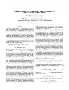
The multivariate version of the normal distribution will probably be very recognizable to those familiar with the univariate version. The surface shown in figure 3.3 provides an illustration of the probability density function (PDF) of the standard normal 26
0.20 0.15 0.10 0.05 0.00
3 2 1 -3
-2
0 -1
0
-1 1
2
-2 3 -3
Figure 3.3: A Multi-variate normal distribution. The points on the plane indicate samples in two-dimensional space. The surface above the plane displays the corresponding probability density function (PDF). The ellipse on the plane is a contour line indicating constant density, and corresponds to one standard deviation.
distribution over two variables. The familiar bell shape is clearly visible, although it is now three dimensional. One hundred sample points drawn randomly from the distribution have been plotted on the plane below the surface, and you can see that they are much more densely packed near the origin (which is also the mean) than out toward the edges of the distribution. An ellipse (which in this case would actually be a circle if viewed from above) has also been plotted on the plane, among the sample points. This is a contour line along which the distribution has equal density. The specific ellipse plotted corresponds to one standard deviation. If it is not clear what this means, consider the following. If we were to create another plane that passes through the origin and was perpendicular to the plane in the figure, it would bisect the surface. The cross section produced would be the familiar univariate bell curve. We could also determine the locations on either side of the mean along that cross-section that indicate one standard deviation. 27
3 2
!
!
! !
1
! ! !
!
!
!
0
!
−1
y
!
!
! !
! !!! ! !
!
!
!
! ! ! ! ! ! !!! ! ! !! ! !! !! ! ! !
! !! !! ! ! ! !! ! ! ! ! !!!! ! ! ! ! ! ! !! ! ! ! ! ! !! ! ! ! ! ! !
!
!!
! !
!
!
!
−2
!
! ! !
−3
!
!
−3
−2
−1
0
1
2
3
x
Figure 3.4: A nonsymmetric multivariate normal distribution. The points indicate randomly generated samples and the ellipse is a density contour corresponding to one standard deviation.
No matter what bisecting plane we chose, these locations will always lie directly on the ellipse. While the distribution shown in figure 3.3 is radially symmetric (the same in every direction relative to the center), not all multivariate normal distributions have this quality. In other words, sometimes a multivariate normal distribution can be longer than it is wide. Figure 3.4 provides an example, although without the PDF surface in this case. Note that the ellipse drawn is no longer circular. Each cross section of the corresponding PDF would still produce a univariate normal bell curve, but the variance of the curve will be different depending on where the cut is made. Also note that the orientation of the distribution does not necessarily lie along one of the standard basis vector (i.e. x, y, z, etc), and so any representation of multivariate variance must be able to represent these rotations as well. Clearly there is more to the notion of multivariate variance than can be captured in a single number. 28
3.3.2
Covariance Matrices
One common way to represent multivariate variance is as a covariance matrix. Their main advantage is that they can be used in multivariate equations in much the same way that univariate variance can be used in univariate equations. A covariance matrix takes the form of an m × m matrix, where m is the number of variables or traits in our case. The function Var calculates variance as a covariance matrix, and is defined as follows:
cov(x1 , x2 ) var(x1 ) cov(x2 , x1 ) var(x2 ) Var(x) = .. .. . . cov(xm , x1 ) cov(xm , x2 )
. . . cov(x1 , xm ) . . . cov(x2 , xm ) . ... .. ... var(xm )
(3.5)
where x is a set of vectors [x1 , x2 , ...xm ] describing the entire population of samples, and xi is a vector of scalar values containing all the sample values for the ith variable. The term covariance matrix can be somewhat confusing, because in this case we are actually using it to representing just variance. The term “covariance” is used to describe these matrices because the non-diagonal elements of the matrix are calculated using the covariance function. These covariances end up describing any diagonal aspects of the distribution. In a sense, they can be thought of as describing the rotations away from the standard basis vectors. To add to this confusing terminology, covariance matrices can also be used to define the multivariate form of covariance. In this case it is called a cross-covariance
29
matrix. The equation for multivariance covariance is defined as follows:
cov(x1 , y1 ) cov(x1 , y2 ) cov(x2 , y1 ) cov(x2 , y2 ) Cov(x, y) = .. .. . . cov(xm , y1 ) cov(xm , y2 )
. . . cov(x1 , ym ) . . . cov(x2 , ym ) . .. .. . . . . cov(xm , ym )
(3.6)
where again x is a set of vectors [x1 , x2 , ...xm ] describing the entire population of samples, and xi is a vector of scalar values containing all the sample values for the ith variable. The second parameter y is defined just as x is, but describes a different population. Univariate covariance describes how two variable vary together. In much the same way, the Cov function describes how two sets of vectors vary together. This produces a measure of similarity between the vectors in x and the corresponding vectors in y. For example, if x and y are identical, the resulting covariance matrix will be the same as both Var(x) and Var(y) (i.e. Cov(x, y) = Var(x) = Var(y)). On the other hand, if the vectors in x and their corresponding vectors in y are unrelated, all the elements of the resulting cross-covariance matrix will likely contain values that are close to zero. This is true even if x and y are drawn from the exact same distribution (i.e. Var(x) = Var(y)).
3.3.3
The Multivariate Form of the Variance Equation
Creating a multivariate version of the variance equation is really relatively simple at this point. As mentioned earlier, each φi and φ�j now represents a vector of traits. The multivariate forms of Var and Cov operate on these vectors, and produce covariance matrices in return. Otherwise, the form of the equation remains essentially the same. 30
If we define the following covariance matrices: Q = Var(φ), P = Var(φλ ), O = Var(φ� ), G� = Cov(φ�λ� , φλ ), and D = Var(φ�λ� − φλ ), we can then rewrite equations 3.3 and 3.4 as follows: O = 2G� + D − P
(3.7)
O = Q · PQ−1 [2G� P−1 + DP−1 − I],
(3.8)
where I is the identity matrix. In standard quantitative genetics theory, the G and P matrices are used frequently, as can be seen in multivariate response-to-selection equation (equation 2.2). As was discussed in section 2.1, heritability can now be thought of as the covariance matrix GP−1 . It is important to note that I have defined a slightly different form of the G matrix that I call G� . Simply put, G = τ G� , where τ is the number of parents per offspring. This really just goes back to the discussion earlier in this chapter. The version of heritability in my equation (G� P−1 ) should be thought of as heritability from a single parent. The effects of selection on population variance are now described by the matrix PQ−1 , perturbation is defined by the matrix DP−1 , and heritability is defined by G� P−1 . There is one other relationship that can be drawn from these equations, the one between the O and P matrices (i.e. OP−1 ), which I will discuss further in the next section.
3.3.4
Two Forms of Heritability
Estimation of Distribution Algorithms (EDAs) were developed based on observations drawn from quantitative genetics theory [M¨ uhlenbein and Paaß, 1996]. Since then the EDA community has moved towards the heuristic that the offspring population 31
distribution should be similar to the parent population distribution [Pelikan et al., 2000]. This has turned out to be an effective strategy, and has served the community well. This is essentially achieved by comparing the O and P matrices, which is what the term OP−1 does. Since OP−1 is a measure of how similar the parent and offspring populations are, rather than how similar the individuals are, I will refer to it as “population heritability”. Both forms of heritability that we care about – standard heritability (G� P−1 ) and population heritability (OP−1 ) – are useful for analyzing and diagnosing reproductive operators. The re-derivation of the variance equation has identified the new term that I refer to as perturbation (DP−1 ), which will also prove useful, as we will see. Now that we have identified the aspects of reproductive operators the we wish to observe, we need to develop methods for measuring and tracking them during an EA run. This is what we will explore in the next chapter.
32
Chapter 4: Analysis Methods Based on Quantitative Genetics To review, the goal of this research is to assist practitioners in customizing EAs for novel problems. At a very high level, the plan is to examine how the population traverses the search space from generation to generation, identify the learning biases associated with the reproductive operators, and check to see if they are consistent with a well functioning EA. We can then use this information to diagnose problems with the customized EA components. This chapter lays out some of the details of this plan. These include approaches to quantifying the search space traits, statistical tools for testing the heritability of traits, and various types of plots that can provide insight into the internal workings of an EA.
4.1
Quantifying the Search Space
The way practitioners identify phenotypic traits that quantify the search space will be crucial to the success of this approach, and it may not always be obvious what to measure. Unfortunately there cannot be any generally defined set of traits. New traits will need to be determined for each new class of problem. Here I provide some advice about identifying what phenotypic traits to measure, and how to measure them. The most important thing to remember is that each trait should define some important quality of the individual in the phenotypic landscape. What this means is 33
that the value of a trait should have an effect on the fitness of the individual. The design of phenotypic trait measures is similar to designing a fitness function for EA — they are problem-specific, and it is more an art and an iterative process to come up with one or more measurements that capture the important aspects of a problem. Some classes of problem have been well studied, and the important aspects that describe the search space are well understood. Defining traits in these cases is often straight-forward. For example, function optimization problems have been a staple of EC test problems for quite some time [De Jong, 1975,Goldberg, 1989], so much so that they essentially act as the basis by which we view fitness landscapes in general. The fitness function is defined as taking a set of parameters, and each parameter defines a dimension over which the function is defined. Since the values of the parameters are the only things that effect the fitness of an individual, we can consider them to be the phenotypic traits that describe the landscape. For more complex problems like agent domains or machine learning problems, measuring phenotypic traits will be more difficult, and so they make good examples to consider. When ECs are applied to these domains, the solutions often take the form of executable objects (i.e. programs). These could take many forms including rule-sets, neural networks, finite state machines and LISP s-expressions, among other representations. Many such problems can be solved using any of the representations just mentioned. One of our goals is to create a representation independent description of the fitness landscape, so a good set of traits should be usable with any of these representations without changing how the traits are measured. There are a number of issues that should be kept in mind when devising a set of traits. Considering how to balance these different properties will help one to think about how to proceed with this design process.
34
4.1.1
Issues
Coverage/Completeness Ideally we would like to develop as complete a set of traits as possible. By “complete” I mean that we would like to have a set of traits that describe the whole phenotypic search space as well as possible. Another way of viewing this is to ask “Do the traits that we have uniquely define an individual?” Previous applications of quantitative genetics to EAs have used fitness alone, providing a very limited and incomplete view of the nature of the fitness landscape. Part of the problem was that individuals that are very different can have the same fitness. Similarly an incomplete set of traits can fail to illuminate certain important aspects of a problem. Machine learning problems are particularly susceptible to this issue because generalization is a critical part of the learning process. We expect our systems to be able to handle new situations that they never faced during training. One way address this issue is to create traits that are, in a sense, general too. Traits that measure a set of behaviors that all fall into a broad category will be able to achieve the best coverage of the search space. For example, trying to measure behaviors at a high level instead of response to stimuli at a low level, creates an opportunity for more general traits. This may require some imagination as well as some insight into the problem domain itself. It is difficult to offer advice as to how one can recognize when their trait set is incomplete. Asking the question mentioned above about uniqueness of individuals seems to be a good starting point. It may be wise to ask oneself this question throughout the design and implementation process. If we fail to find a set of traits that provide complete coverage, all is not lost. One convenient quality the quantitative genetics equations is that they degrade gracefully 35
when given an incomplete set of traits. In other words, all the equations are still completely accurate, at least within the context defined by that subset of traits. Of course we will be looking at an incomplete picture of what is going on, and crucial information could be missing. Unnecessary traits Unnecessary traits can come in a number of forms. For example, they may just not affect the fitness, they may always by constant, or they may be so closely correlated with another trait that they essentially are measuring the same thing. These can be problematic because they can affect our ability to perform the necessary calculations. I will discuss matrix computation issues in more detail in section 4.2. It is important to realize that some of these issues can be avoided if we are careful in how we choose our traits. Linking Phenotype to Genotype If one’s goal in using these tools is to identify and fix problem in an algorithm, then it becomes important to identify connections between the traits and any aspects of the representation or reproductive operators that are affecting those traits. The more abstract the traits are, the more difficult this becomes, and so very low-level descriptions of behaviors may be more appropriate to achieve this. Unfortunately, this can creates a conflict with the issue of trait completeness described above. There I suggested that higher-level traits may be better for getting the best landscape description possible. For example, consider a problem where we are trying to teach an agent to track another agent without being detected. A high-level set of traits might measure things like: how much distance an agent keeps between itself and the target, the length of time that it is able to maintain surveillance, and 36
the number of times it is detected. These traits may be ideal for covering all the skills that are necessary for describing the fitness landscape, but they may not be very helpful for identifying what aspect of a representation or reproductive operators are problematic for effective learning in this domain. Such connections would be tenuous at best. At the other end of the scale, a low-level phenotype (conceptually, at least) might be something as simple as the input-output map that exactly describes the actions the agent would take for any given set of inputs. Here we have a much better chance of relating such information to the representational structure, and the effects of the reproductive operators. Unfortunately, it becomes much more difficult to define a complete set of traits. Such a set would have to describe the entire map, and this might mean thousands of traits, one for each possible input. The only viable option is to create sample sets of inputs that are hopefully representative in some way. If one can define enough traits to get a reasonable sampling of the input space, or identify important samples that yield particularly valuable information, then this approach could still be useful. Multivariate Normality One important aspect of defining phenotypic traits that should be addressed are the assumptions that are built into the quantitative genetics equations. Most important among these is the expectation that the underlying distributions are normal, or at least close to normal. In order to achieve this, biologist often remap the traits to another scale using a variety of transformation functions [Falconer and Mackay, 1981, Hartl and Clark, 2007]. There are a few qualities that any remapping function should have. First, it should be a one-to-one mapping so that no information is lost. Also, if comparing 37
one generation against another, the functions should be the same in both cases. In general this means that the same mapping functions should be used throughout the entire run of the algorithm. Ultimately, it is ideal if the combined set of remapped traits is multivariate normal. In practice however, making sure each trait alone is normally distributed is often enough. Some functions are very commonly used, such as taking the exponent of a trait. We have found that the sigmoid function is effective at reducing or eliminating outliers, which can be problematic. There are also some techniques, like Box-Cox estimation [Box and Cox, 1964], that may be able to provide general, and somewhat automated, mapping solutions.
4.2
Computational Issues with Matrices
Up to this point I have implied that covariance matrices are equivalent to normal joint probability distributions. It should be noted that not every M × M matrix describes a valid distribution. In order to do so, a matrix must have two properties. The first is that it must be a Hermitian matrix. For our purposes, this essentially means that the matrix is symmetric, and that the eigenvalues are real-valued (i.e. not imaginary). The second property is that none of the eigenvalues can be negative. This type of matrix is referred to by two equivalent names: positive semidefinite and nonnegative definite. We can expect the P, O and D matrices to have this quality. There is an important degenerate case for positive semidefinite matrices that occurs when a matrix is singular. This means that the determinant is zero, and since the determinant is essentially equal to the product of the eigenvalues, one or more of the eigenvalues is therefore zero as well. Such a matrix defines a probability distribution that has no density, and it causes problems when performing certain calculations, like 38
finding the matrix inverse (e.g. P−1 ). A matrix in which all eigenvalues are greater than zero is called positive definite, and if possible, we would like to work with such matrices whenever possible. Poorly chosen traits are one factor that can lead to singular matrices. There are at least two situations that are likely to cause such problems. The first occurs when selecting traits that show little to no variance, and the second involves selecting two traits that essentially measure the same thing, or are at least very highly correlated. Sometimes calculation errors can result in non-positive definite matrices also (matrices with negative eigenvalues). These may be caused by roundoff error, or these can occur when the number of samples (individuals in the population) is relatively small. To deal with calculation errors, I use the techniques described by [Opgen-Rhein and Strimmer, 2007], that was implemented in the corpcor package for the R statistics program [Schaefer et al., 2010]. Simply stated, the idea is to create a covariance matrix that describes an oversized probability density function for the given data, and then iteratively shrink the distribution down until it roughly covers the appropriate region. With this approach, the shrinkage can be halted in any direction before the associated eigenvalue becomes negative or zero. I use this package in my analyses to calculate all covariance matrices that are the result of the Var function (equation 3.5) as well as any associated inverse matrices. While the matrix version of Var should theoretically always result in a positive semidefinite matrix, the same cannot be said of the cross-covariance function Cov (equation 3.6). This function can result in perfectly valid negative definite matrices. This means we have no guarantee that the G� matrix will be positive semidefinite.
39
4.3
Matrix Similarity Metrics
When biologists consider the multivariate notion of heritability, they tend to think in terms of the degree of similarity between the two probability distributions that P and G describe. The more similar the two matrices are, the closer the heritability will be to the identity matrix. Matrix comparisons are often performed using statistical techniques like Common Principle Component Analysis [Flury, 1988, Game and Caley, 2006]. In preliminary experiments with CPCA, I found its output to be too course grained to be useful as a diagnostic tool. This has led me to consider other approaches. I had a number of goals in mind for the metric that I wanted to use. 1. Scalar: The resulting value produced by the metric should be a scalar number. Matrices are too complex to analyze easily. Having scalar values that can be plotted for each generation makes it much simpler to create plots that can be understood, even if the metric is not perfect. 2. Identity: If a matrix is compared with itself, the resulting scalar value should equal one. In other words, m(A, A) = 1, where m is the metric function and A is a matrix. 3. Addition: The scalar results of the metric should retain a similar additive quality to those of the original matrices that produced them. In other words, if AX−1 + BX−1 = I, then m(A, X) + m(B, X) = 1. The hope is that this will provide some insight into the interplay between various matrices that will help with diagnosing problems. 4. Tractable: It is important that the calculations for the metric are tractable in a wide variety of situations. If this is not the case, then some EAs and problem 40
�� ����
��������� �
Figure 4.1: Geometric interpretation of the trace function.
domains could become impossible to analyze using such a comparison metric. I have developed two metrics that come close to achieving the goals above. Both are based on the matrix trace function.
4.3.1
The Trace Function
The trace function of a matrix is defined as follows:
tr(A) =
M �
aii ,
(4.1)
i=1
where A is an M × M matrix, and aij refers to the element of the matrix at row i and column j. It is essentially a sum of all the diagonal elements of the matrix. It is also equal to the sum of the eigenvalues, so it is essentially the sum of all the variation in the matrix. The trace function provides a useful basis for a similarity metric because it has 41
an intuitive geometric interpretation. Consider the M dimensional hyper-rectangle defined by the the eigenvectors of the matrix. Now consider a vector drawn from the origin to a corner of this hyper-rectangle. The trace function returns a value equal to the length of this vector. See figure 4.1 for an illustration. In previous work I had developed a metric that was based on determinants [Bassett and De Jong, 2011]. Determinants are particularly susceptible to problems related to singular matrices. I have found the trace function to be much more robust to these problems, thus making a better basis for a metric.
4.3.2
Similarity Metrics
The first metric I will use is defined as follows:
m1 (A, B) =
tr(AB−1 ) M
(4.2)
where A and B are both M × M covariance matrices. This means, for example, that our scalar metric for heritability will be tr(G� P−1 )/M . This metric meets the first three of the goals I described above quite well. First, the result is a scalar. Second, m1 (A, A)/M = tr(I)/M , which is guaranteed to equal 1. And third, it is not hard to show that the additive quality I discussed holds true for this metric. The one concern about this metric is in regards to tractability. As discussed earlier, calculating the inverse of a matrix can sometimes be problematic. Because of this, I decided to define a second metric that would be less susceptible to computational
42
problems. It is defined as follows:
m2 (A, B) =
tr(A) tr(B)
(4.3)
Using this metric, heritability would be measured as tr(G� )/tr(P), population heritability becomes tr(O)/tr(P), and perturbation becomes tr(D)/tr(P). With this metric I have made a trade-off. Tractability is improved, but I have sacrificed a certain amount of accuracy in the calculations in order to achieve it. In other words, the “additive” quality that I described as a goal no longer holds under all circumstances. Fortunately all the other goals are still met.
4.4
Plots
4.4.1
Matrix Ellipse Plots
Covariance matrices are not easily interpreted by just looking at the numbers. One approach that can give some insight is to plot density contours associated with a covariance matrix as ellipses. As described in section 3.3.1, an ellipse can represent one standard deviation of the multivariate normal distribution. Plotting ellipses from multiple distributions on the same plot also provides a method for visually comparing matrices. The ellipse in figure 4.2 is an example of just such a plot. What follows is a brief description of how to calculate and plot one of these ellipses. We begin with the matrix A for which we want to plot an ellipse. Our first step is to use the singular
43
3 2
!
!
! !
1
! ! !
!
!
!
0
!
−1
y
!
!
! !
! !!! ! !
!
!
!
! ! ! ! ! ! !!! ! ! !! ! !! !! ! ! !
! !! !! ! ! ! !! ! ! ! ! !!!! ! ! ! ! ! ! !! ! ! ! ! ! !! ! ! ! ! ! !
!
!!
! !
!
!
!
−2
!
! ! !
−3
!
!
−3
−2
−1
0
1
2
3
x
Figure 4.2: A matrix ellipse plot shows an ellipse representing one standard deviation of the joint probability distributions described by the covariance matrix. This ellipse is projected onto a 2 dimensional plane.
value decomposition (SVD) function to calculate a transformation matrix.
B = svd(A)
(4.4)
The SVD function is essentially the matrix equivalent of the square root function, so the new matrix B now represents standard deviations instead of variances. While the B matrix is defined for all the traits, an ellipse plot has to be plotted on a 2 dimensional surface, so we will need to reduce it to represent only a subset of entire matrix. The simplest approach is to choose only 2 traits to plot. This has the effect of projecting the entire ellipsoid onto the plane defined by those two trait dimensions. For example, if we are most interested in the traits t1 and t2 , we can create a subset
44
of the matrix as follows:
bt1 ,t1 C= bt2 ,t1
bt1 ,t2 , bt2 ,t2
(4.5)
where bi,j refers to the element of matrix B at row i and column j. Finally, we create a set of points that are evenly spaced around a unit circle, and then multiply these by the transformation matrix C. The equation for the points is as follows,
cos( 2πi ) N
xi pi = = C 2πi yi sin( N )
(4.6)
where i ∈ [1, 2, · · · N ], and N is the total number of points generated. These points can then be plotted as a polygon, giving us an approximation of an ellipse, such as the one in figure 4.2.
4.5
Eigenvalue plots
As mentioned earlier, when transforming all the variation in a matrix into a single scalar value, a lot of information is lost. For example, by using the trace function, we are summing all the eigenvalues together. This means that two very different matrices could actually have the same scalar value associated with them. Sometimes it may be useful to get more detailed information about the state of the matrix, while still avoiding all the detail. One technique that allows us to get achieve this middle ground is to examine and compare the individual eigenvalues instead of summing them together. In general I will be plotting the trace values of the various matrices (P, O, etc.), 45
or the m1 or m2 metrics for perturbation and both forms of heritability for each generation in the run. When I need more detailed information, I will also generate eigenvalue plots for these matrices. The X axis will indicate the generation of the algorithm and the Y axis will indicate the magnitude of the eigenvalue. For a single N × N matrix, N lines will be plotted, one for each eigenvalue. This plot will allow us to see how much distortion exists in the matrix. If all the lines have very similar values, then the distribution is essentially spherical (equal variance in every direction). But when eigenvalues are quite different from one another, it means that the variances are much higher in some directions than in others. This indicates a distortion, and may be useful for identifying when the distribution is changing shape, even if the total amount of variance remains the same. With the various metrics and tools outlined in this chapter, we now have what we need to examine the internal behavior of an EA as it proceeds through a run. In the next chapter we will apply these tools to some simple EAs on some well understood function optimization problems, so that we can get a sense for how they actually behave in specific situations.
46
Chapter 5: Methods Validation with Function Optimization For many, equations do not provide enough of a handle for really understanding a theory. A set of simple examples can often expose some of the insights that a theory has to offer. This chapter is devoted to working through some commonly used EAs when applied to some relatively simple problems. I expect this will help some to attain an intuitive understanding of the equations from chapter 3. These experiments will also give us a chance to validate that the tools are, in fact, showing us what we would expect to see. The class of problems we will be looking at is function optimization. The particular advantage here is that fitness landscapes become very easy to visualize. Our very notion of a fitness landscape is almost synonymous with a multivariate function, and these are the first types of problems that many who are learning about EAs will see.
5.1
Random Search
Before we look at a proper EA, as a baseline we will examine an algorithm that is less complex. The random search algorithm is often used as a baseline of comparison in EA research. It also offers us some interesting insights as it represent an extreme case in the spectrum of possible evolutionary behaviors. When a random search is performed, a series of randomly generated potential solutions are examined one by one. The only information that is retained is the best solution found so far; in other words, the solution with the best fitness. Random 47
potential solutions can be generated in a number of way, but typically the parameter values that define a solution are drawn from a uniform distribution of the set of all possible values. When one possesses some specific knowledge of the search space, values can be drawn from a subset of possible values, thus allowing for a more focused search.
5.1.1
EA Framework
In order to adapt the random search algorithm for use with my tools I essentially need to implement it within an EA framework. This is easy to do with just a couple of simple changes. First, we use an EA with non-overlapping generations, along with deterministic selection. In other words, every individual is selected once, and only once, for reproduction. This has the effect of providing no selection pressure. The second step involves creating a new reproductive operator that just generates new individuals completely randomly. No genetic information is passed from parent to offspring.
5.1.2
The Problem Function
The choice of a test problem is not really important, since this algorithm has no bias to guide it toward better solutions. This means that the only important factor is the overall distribution of fitness values among the potential solutions. Nonetheless, we will begin with a problem that is fairly simple for an EA to solve. Specifically, we will examine what is often referred to as the sphere function:
f (X) =
N � i=1
48
x2i
(5.1)
where X is a vector of size N and xi is the ith component of X.
5.1.3
Representation
Individuals will be represented as a string of real-valued numbers. These numbers will be referred to as genes. During initialization for this problem, all genes are generated within the range [−5.12, 5.12). Due to the way our random search reproductive operator works, this also means that all genes will always fall within this range. This constraint may not be enforced for other reproductive operators we look at later in this chapter, though. In this experiment, we use N = 10. This number is chosen somewhat arbitrarily, but I wanted to have enough dimensions so that examining every possible gene-gene combination would be an involved process.
5.1.4
Defining Traits
When defining traits, our goal is to define a set that best describe the search space. For function optimization problems, the most straight-forward conceptualization of the search space is that of the parameter space. In other words, the inputs to the fitness function. So for equation 5.1, each parameter xi will also be treated as a quantitative trait. Traits will be defined similarly for all problems in this chapter.
5.1.5
Algorithm Behavior
Using a population size of 50, the algorithm was run for 200 generations. This means that 10,000 individuals were examined during the course of each run. To get a sense for how the algorithm performs, see the the best-so-far curve in figure 5.1. This plot was averaged over 10 runs, and the whiskers indicate the 95% confidence intervals for 49
10
40
5
parents offspring P ellipse O ellipse
0
−10
−5
0
Trait 2
20 10
Fitness
30
Random search
0
50
100
150
200
−10
Generations
−5
0
5
10
Trait 1
Figure 5.1: Best-so-far plot for the random search algorithm Results are averaged over 10 runs, and the whiskers represent 95% confidence intervals.
Figure 5.2: Scatter plot of parent and offspring traits during random search. Points are projected onto a plane defined by two traits.
the average. As we would expect with such an undirected search, there appears to be plenty of room for improvement. To understand what is happening inside the algorithm, we can plot some of the operator’s characteristics by applying the metric m1 to them. Before we do that, though, we will take a more detailed look at the populations from a phenotypic perspective so that we can get a feel for how those metrics are calculated, and what they are really indicating. Figure 5.2 shows a scatter plot of population traits at the first generation of one of the runs. There are 10 traits in our experiment, but this type of plot only shows two. This is mainly because it is too difficult to visualize more than two dimensions at a time. This means that all the points are projected onto the plane defined by traits 1 and 2. Because we know that our landscape has a high degree of symmetry, 50
we can expect to see the same thing no matter which two traits we choose. With a different landscape we would have no such guarantee. The plot shows both the selected parents and the resulting offspring. In addition, I have plotted the ellipses for the covariance matrices P and O that are calculated from these populations. These ellipses indicate density contours that are one standard deviation from the mean. As you can see, the ellipses are very similar in size. The centers of the ellipses are placed at the population means, which is why they look offset from each other. It should be noted, though, that the mean has no effect on the metrics that are ultimately calculated. These metrics only compare the variances of the distributions. The scatter plot does not give us any sense of the relationship between parents and offspring. In figure 5.3 I replot these two populations, but with lines connecting each parent with its offspring. Of course it is very difficult to make any sense of this plot. Figure 5.4 recasts this information in a way that is hopefully easier to read, while still being intuitive. Imagine taking each line in figure 5.3 and translating it so that the parent is at the origin. This gives a sense for how much variation in the offspring population is a result of the reproductive operators. This is what the D matrix represents, and is calculated using the full N dimensional versions of the points shown in the plot. I have plotted the ellipse for D in figure 5.4 as well. Now we put these pieces together so that we can start to get a picture of how our algorithm is behaving. Figure 5.5 plots all three of the ellipses we have seen so far for the first generation. As I mentioned before, the P and O ellipses are very similar in size. Interestingly though, the D ellipse is much larger. While the scatter plots and ellipses provide us with useful information in a very intiuitive form, they become quite difficult to use when one cannot rely on their landscape having a high degree of symmetry, as we have done here. You would have 51
10 10
offspring − parent D ellipse
−10
−10
−5
−5
0
Trait 2
0
Trait 2
5
5
parents offspring relationship
−10 −10
−5
0
5
−5
0
5
10
10 Trait 1
Trait 1
Figure 5.4: Scatter plot of offspring relative to their parents during random search. Parent trait values are subtracted from offspring values. Ellipse indicates one standard deviation.
10
Figure 5.3: Scatter plot of parents and offspring with connections during random search algorithm. A line is drawn from every offspring to its parent.
0 −10
−5
Trait 2
5
P ellipse O ellipse D ellipse
−10
−5
0
5
10
Trait 1
Figure 5.5: Standard deviation ellipses for P (parents), O (offspring) and D (difference) matrices for random search. 52
to create such a plot or all trait combinations to be confident that you knew what was really going on with the populations. This is where the metrics described in section 4.3 become useful. They aggregate critical information about each matrix into a single number so that only a few plots are needed. In figure 5.6 I plot the trace of the four matrices (P, O, D and G� ) from equation 3.7 throughout the run of our random search algorithm. To be more precise, what is plotted are the traces averaged over 10 runs. The whiskers indicate 95% confidence intervals. Here we see much of the same information we learned from the scatter and ellipse plots. It may be a little difficult to see from the plot, but lines for P and O matrices are plotted right on top of one another, confirming that the variation in the two populations is very similar. We can also see that they remain the same throughout the runs. In other words, our populations are not converging at all in phenotypic space, but instead continue to search the entire search space throughout the run. Since we are not using any selection pressure this should not come as a surprise, but as we will see in the next section there is more to it than that. Instead of trying to explain the D and G� curves on this plot, consider figure 5.7, where we plot m1 metrics for both forms of heritability, as well as perturbation. As discussed before, in a multivariate analysis these concepts are best described using the matrices G� P−1 , OP−1 and DP−1 . Here we have reduced these matrices to scalars using the m1 metric, while hopefully retaining useful and important information. We can see a number of things from this plot. First, the population heritability remains close to 1, indicating the the parent and offspring populations remain similar throughout the runs. Next we notice that while the heritability is quite small (almost zero), the perturbation is relatively large. This means that the operators are responsible for most of the variation in the population. In our example here, variation in the offspring population can only come from two sources. It is either created by 53
4
300
3
tr(OP!1) 10 Pop. Heritability tr(G'P !1) 10 Heritability tr(DP!1) 10 Perturbation
0
0
50
1
100
2
150
200
250
tr(D) tr(O) tr(P) tr(G' )
0
50
100
150
200
0
10
Generations
30
40
50
Generations
Figure 5.6: Matrix trace curves of P, O, D and G� during random search without selection. Results are averaged over 10 runs.
Figure 5.7: Trace of matrix ratios for random search algorithm without selection. Results are averaged over 10 runs.
4
300
20
3
tr(OP!1) 10 Pop. Heritability tr(G'P !1) 10 Heritability tr(DP!1) 10 Perturbation
0
0
50
1
100
2
150
200
250
tr(D) tr(O) tr(P) tr(G' )
0
50
100
150
200
0
Generations
10
20
30
40
50
Generations
Figure 5.8: Matrix trace curves for random search with 50% trunction selection. Results are averaged over 10 runs. 54
Figure 5.9: Trace of matrix ratios for random search with 50% trunction selection. Results are averaged over 10 runs.
the reproductive operators (perturbation), or it is retained from the variation that already existed in the original parent population (heritability). So we see that with our random search operator, populations retain no variation from previous generations. Of course this makes sense, since each new individual generated is completely independent of its parent.
5.1.6
Adding Selection
Next we take a this algorithm one step closer to being an EA by adding some selection pressure. In fact I have added quite a high selection pressure in order to exaggerate the effects and make them more obvious. I have used truncation selection, with a truncation ratio of 50%, and therefore the bottom 50% least fit individuals never get to reproduce. As we know, individuals are always generated within the same bounds, no matter what form the population of selected parents takes. We should expect then that adding selection will not have any effect on the performance of the algorithm. This is verified by the best-so-far plot in figure 5.10. The curve for 50% truncation is not significantly different from the curve representing no selection pressure. The traces of the matrices P, O, D and G� are plotted for this version of random search in figure 5.8. Now we see that the P matrices, which are the covariance matrices associated with the selected parent populations, are much smaller throughout the run. They are smaller than they were in the previous experiment shown in figure 5.6, and they are also smaller that the corresponding O matrices in this experiment. One way to view selection is as a mechanism to constrain the search to more promising parts of the search space. From this perspective, selection’s job is essentially to exploit existing knowledge about the landscape. In this experiment, selection is doing its job, but this is not enough. The reproduction operators need to provide 55
40 20 0
10
Fitness
30
No selection 50% Truncation
0
50
100
150
200
Generations
Figure 5.10: Best-so-far plot of random search algorithm with and without selection. Results are averaged over 10 runs. The whiskers indicate 95% confidence intervals.
support in order to maintain those constraints. In other words, the offspring population should occupy the same general part of the phenotype space as the selected parent population. Said another way, the population heritability (OP−1 ) needs to be as close to the identity matrix as possible. If this were the case, then tr(OP−1 )/N would equal 1. As we can see in figure 5.9, this is not the case. One simple approach to maintaining the constraints set by selection is to retain some of the variation of the selected parent population in the offspring population. This means that operators with good heritability (G� P−1 ) should be able to achieve this goal. This is why I believe there is a relationship between heritability and exploitation, even though population heritability (OP−1 ) is the better measure of exploitation.
56
5.2
Selection and Cloning
We will consider one more baseline example, which in many ways is at the opposite end of the spectrum from random search. In this case, the reproductive operator creates no variation. Consider an algorithm where the only reproductive operator is cloning. In other words, every offspring produced is an exact copy of the parent. Thus the only thing that changes the composition of the population is selection. In this case I use a rank proportional selection with stochastic universal sampling (SUS) [Baker, 1987]. The result is a selection pressure that is the same as binary tournament selection, but with much less genetic drift [De Jong, 2006, pg. 125]. Looking at figure 5.11, we can see that, as opposed to the random search algorithm, the population definitely converges in phenotype space. Also, the curves for the P and O matrices seem to lie directly on top of one another. The trace of G� is not plotted on this graph, because it also lies directly on the curves for P and O, and makes the plot too difficult to read. Another thing to notice is that the trace of the D matrix remains at zero throughout the run. In figure 5.12, we can see that despite the fact that the populations are converging, the metrics for perturbation and both forms of heritability remain fairly constant throughout the run, at least until generation 10 or so. At this point the parent population has converged to a single point in phenotype space, thus eliminating all variance, and making these ratios undefined. Most importantly though, when we compare figure 5.12 with its counterpart in random search, figure 5.7, we can see that both maintain values near 1 for population heritability, but they do so in very different ways. In the random search algorithm, all phenotypic variation is derived from perturbation, and none is retained through
57
80
heritability, but in the cloning algorithm, just the opposite is true.
4
tr(O) tr(P) Pop. Heritability tr(G' ) tr(P) Heritability tr(D) tr(P) Perturbation
0
0
1
20
2
40
3
60
tr(P) tr(O) tr(D)
0
5
10
15 0
Generations
5
10
15
Generations
Figure 5.11: Matrix trace curves for cloning-only EA on the sphere function. Results are averaged over 30 runs. Whiskers indicate 95% confidence.
Figure 5.12: Trace of matrix ratios for cloning-only EA on the sphere function. Results are averaged over 30 runs.
Despite the fact that the cloning-only algorithm is able to converge on a solution, its performance is really not very good, as can be seen in figure 5.13. This will come as no surprise to anyone familiar with EAs. Without additional variation from the reproductive operators, the algorithm is unable to explore beyond the solutions that exist in the initial population. For that matter, neither of these algorithms perform particularly well. This highlights the fact that, while both perturbation (exploration) and heritability (exploitation) are important, neither one alone is sufficient to create a high performance search algorithm. The best algorithms (and operators) will have to achieve a proper balance between the two.
58
40 30 20 10
Fitness
0
Cloning and rank selection
0
50
100
150
200
Generations
Figure 5.13: Best-so-far curve for cloning-only EA on the sphere function. Results are averaged over 30 runs. Whiskers indicate 95% confidence interval.
5.3
Gaussian Mutation
Now that we have examined two baselines at the extreme ends of the spectrum, we will look at a relatively simple EA to see how it behaves in comparison. I have chosen an EA that uses just Gaussian mutation with a fixed standard deviation, along with some form of selection. For each gene in the genome, the mutation operator adds a number drawn from from a Gaussian distribution. The selection operator will again be the SUS rank proportional selection, and the fitness landscape will be the Sphere function (equation 5.1) with N equal to 10. For this experiment, I will compare the behavior of the algorithm using varying amounts of mutation. Specifically, I use standard deviation values of 0.05, 0.1 and 0.2. Figure 5.14 shows the best-so-far curves for the differing amounts of mutation. As we can see, larger amounts of mutation allow the algorithm to zero in on the
59
solution much more quickly. But when we zoom in on the curves toward the end of the runs, as in figure 5.15, we can see that better solutions can be found when using
1.5
0.0030
the smaller amounts of mutation.
Sigma 0.05 Sigma 0.1 Sigma 0.2
0.0
0.0000
0.5
0.0010
Fitness
Fitness
1.0
0.0020
Sigma 0.05 Sigma 0.1 Sigma 0.2
0
20
40
60
80
0
100
20
40
60
80
100
Generations
Generations
Figure 5.14: Best-so-far curves for Gaussian mutation EA with 3 different standard deviations on the sphere function.
Figure 5.15: The same best-so-far curves as in figure 5.14, but zoomed-in to allow easier comparison of the final results.
We will start by looking at some of the ellipse plots for one of EAs to get a sense for what is happening. Figures 5.16 through 5.19 show a progression for a single run of the EA at generations 1, 6, 10 and 199. These were done with a mutation standard deviation value of 0.2. There are a few things we can notice here. First, the D ellipse remains the same shape and size throughout the run. This is the result of the fixed standard deviation value for the Gaussian mutation. The second thing we can see is that the P and O ellipses are very similar throughout the runs, although a close examination of generation 199 (figure 5.19) will show that they do diverge a bit towards the end of the run. Also, the population has converged down to an area that is similar in size to the D matrix ellipse. In fact what 60
has happened is that the amount of variation provided by the Gaussian mutation has come into balance with the reduction in variation caused by selection. Once this occurs, the population can no longer converge, and the search turns into something more closely resembling random search within that small area. Finally, we can see that by generation 10 (figure 5.18), the population has largely converged on an area that is not near the optimum, which is at the origin. From that point forward, the algorithm must explore beyond the bounds defined by the population in order to make its way to the optimum. Instead of pouring through all these plots of the populations in trait-space, we can look at our simplified metrics. In figure 5.20, I plot the trace values for the D matrices throughout the runs. Each line is averaged over 10 runs. Since we are using a fixed standard deviation for the mutations, what we see is that the variance in the D matrix also remains fixed throughout the run, just as we saw with the ellipse plots. Looking at figure 5.21, we see that the phenotypic variation among the selected parents decreases in the early part of the runs. As the search proceeds, the population converges on an optima in the search space. Eventually these curves level off, though. This happens somewhere between generation 25 and 50, depending on which curve we are looking at. This leveling off occurs when the loss in variation due to selection and drift begins to balance the increases due to mutation. Putting these two components together, we can examine the amount of perturbation created by the operators, as seen in figure 5.22. Since this measure is a ratio, it describes the amount of exploration relative to the region defined by the population of selected parents. This is why the curves increase over time, even though the mutation standard deviations are fixed. What we see, at least on this fitness landscape, is that higher perturbations tend to lead to faster convergence times. Turning our attention from exploration to exploitation, figures 5.23 and 5.24 plot 61
2
4
P ellipse O ellipse D ellipse
−4
−2
0
Trait 2
0 −4
−2
Trait 2
2
4
P ellipse O ellipse D ellipse
−4
−2
0
2
4
−4
−2
Trait 1
4
Figure 5.17: Standard deviation ellipses for Gaussian mutation EA at generation 6.
P ellipse O ellipse D ellipse
2 0 −2 −4
−4
−2
0
Trait 2
2
4
P ellipse O ellipse D ellipse
4
2
Trait 1
Figure 5.16: Standard deviation ellipses for Gaussian mutation EA at generation 1.
Trait 2
0
−4
−2
0
2
4
−4
Trait 1
−2
0
2
4
Trait 1
Figure 5.18: Standard deviation ellipses for Gaussian mutation EA at generation 10. 62
Figure 5.19: Standard deviation ellipses for Gaussian mutation EA at generation 199.
0.4
0.4
0.0
0.1
0.2
tr(P)
0.2 0.0
0.1
tr(D)
0.3
sigma0.2 sigma0.1 sigma0.05
0.3
sigma0.2 sigma0.1 sigma0.05
0
50
100
150
200
0
Generations
50
100
150
200
Generations
Figure 5.20: Trace of the D matrix for Gaussian mutation EA with 3 different standard deviations on sphere function.
Figure 5.21: Trace of the P matrix for Gaussian mutation EA with 3 different standard deviations on sphere function.
heritability and population heritability respectively. We can see that heritability maintains a consistent value near 1.0 throughout the run for all mutation standard deviations. Population heritability, on the other hand, moves away from 1.0 at different rates for the different mutation standard deviation values. The more quickly it moves away from 1.0, the more quickly it seems to lose its ability to converge on a solution. This emphasizes an important point. Both forms of heritability may be important for diagnosing an EAs behaviors. In fact, ultimately population heritability may be a more accurate measure of exploitation than standard heritability.
63
2.0 1.5 1.0 0.5 0.0
tr(DP!1) 3 Perturbation
sigma0.2 sigma0.1 sigma0.05
0
10
20
30
40
50
Generations
1.5 1.0
tr(OP!1) 3 Population Heritability
1.5 1.0
sigma0.2 sigma0.1 sigma0.05
0.0
0.5 0.0
tr(G'P !1) 3 Heritability
sigma0.2 sigma0.1 sigma0.05
0.5
2.0
2.0
Figure 5.22: Perturbation (tr(DP−1 )/3) for the Gaussian mutation EA with 3 different standard deviations on the sphere function.
0
10
20
30
40
0
50
10
20
30
40
50
Generations
Generations
Figure 5.24: Population heritability (tr(OP−1 )/3) for the Gaussian mutation EA with 3 different standard deviations on the sphere function.
Figure 5.23: Heritability (tr(G� P−1 )/3) for the Gaussian mutation EA with 3 different standard deviations on the sphere function. 64
5.3.1
Side-Effects of Using Fixed Sigmas
With the sphere function, using the same standard deviation on each gene seems perfectly reasonable. When we examine a different fitness landscape though, we see that some problems arise. For example, take the following function which I call the valley function: � � N �� f (X) = |x1 | + 10� x2i ,
(5.2)
i=2
where X is a vector of size N and xi is the ith component of X. The result is a valley that runs the length of the first dimension (x1 ). The valley walls are fairly steep, coming to a sharp edge at the valley floor. The valley floor itself has a gentle slope toward the origin, which is the location of the global minimum. For this problem we will use a value of N = 3 to help exagerrate some of the effects so they are easier to recognize. The same EA from the previous experiment (Gaussian mutation only) was run on this landscape, with a fixed standard deviation of 0.1. The best-so-far curves of this EA are plotted in Figure 5.25, as run on both the sphere function and the valley function. We can see that the performance on the valley function is significantly worse. Figure 5.26 shows the quantitative genetics metrics when run on the valley function. Most interesting is to compare both population heritability (OP−1 ) here, with the sphere function (figure 5.24). The value has increased from approximately 1.3 on the sphere function, to close to 1.7 on the valley function. The metrics do no really provide enough information to diagnose the situation any further, so we will have to try one or two other approaches. Figures 5.27 gives a much clearer view of the problem. Note in this plot that the 65
valley floor is aligned along trait 1, and so it runs along the x-axis. It is important that trait 1 is visualized in this figure in order to see this effect. This provides a further reminder that without the metrics, all trait combinations need to be plotted to be sure of what is happening. In figure 5.27 we see is that as the population converges on a solution, certain dimensions (in this case trait 2, but the same happens with trait 3 also) cannot converge any further because it has reached a limit set by the Gaussian standard deviation in that direction. In other words, the standard deviations are not well tuned to the problem, and as a result it keeps exploring up the sides of the valley instead of along the valley floor, where the fitnesses are better. In particular, this can be seen by the fact that the O ellipse is larger along trait 2 than the P ellipse is. Figure 5.28 gives another view of this effect. Here, at each generation, the OP−1 matrix is averaged over the 30 runs, and the eigenvalues are then calculated and plotted. Recall that the trace function is equal to the sum of the eigenvalues. Also, if the O and P matrices were identical, the eigenvalues should all be close to 1. Instead what we see is that two of the eigenvalues are much larger than 1, while a third seems to be very close to 1. Eigenvalue 3 corresponds to trait 1, which is easily verified by examining the corresponding eigenvector. What this means is that we can improve performance of the algorithm by adjusting the standard deviation in each of the dimensions to something that is appropriate for the particular problem. As we will see though, there are several EA operators which can perform this adjustment automatically.
66
5
1.0
tr(OP!1) 3 Pop. Heritability tr(G'P !1) 3 Heritability tr(DP!1) 3 Perturbation
4 3
0.6
2
0.4
0
0.0
1
0.2
Fitness
0.8
Sphere Valley
0
50
100
150
0
200
10
20
30
40
50
Generations
Generations
Figure 5.26: Heritability, population heritability, and perturbation for Gaussian mutation EA on the valley function.
1.0
5
Figure 5.25: Best-so-far curves for Gaussian mutation EA on the sphere and valley test functions.
Eigenvalue 1 Eigenvalue 2 Eigenvalue 3
2
0.0 −1.0
0
1
−0.5
Trait 2
3
0.5
4
P ellipse O ellipse D ellipse
−1.0
−0.5
0.0
0.5
0
1.0
10
20
30
40
50
Generations
Trait 1
Figure 5.27: Standard deviation ellipses of the P, O and D matrices for Gaussian mutation EA on the valley function at generation 15. 67
Figure 5.28: Eigenvalue plot of the population heritability (OP−1 ) matrix for the Gaussian mutation EA on the valley function. Results are averaged over 30 runs.
5.4
Recombination
Another frequently used reproductive operator, especially within the Genetic Algorithm (GA) community, is recombination. This operator, also referred to as crossover, has some interesting properties that actually balance out the weaknesses of mutation, and so I will spend a little time here examining it. The specific recombination operator I will be examining is called uniform recombination, and it is typically implemented in the following way. After two parents are selected, they are both given to the recombination operator. The operator iterates through the genomes of both parents simultaneously, and with each step i, the genes that occupy location i in each genome are swapped with some probability pswap . The resulting individuals are either passed on to the next reproductive operator (mutation for example), or placed in the offspring population. We begin by examining an EA that uses uniform recombination, but no mutation. It would be unusual to use such an EA in practice, because recombination is known to have trouble maintaining diversity in the population. For this reason, I will use a population size of 1000 individuals instead of 100. I will again be using the SUS rank proportional selection to reduce genetic drift. Finally, the probability of swapping two genes is pswap = 0.5, and the probability of performing recombination is pcross = 1.0. In other words, every individual that is selected will participate in recombination, and none will just be cloned. The genome will again contain 3 genes (N = 3) to make comparisons with certain other experiments easier. Ten runs of the EA were performed on the sphere function. Figure 5.29 gives us a snapshot of the parent and offspring trait values in the first generation of one of those runs. Note that lines are also drawn between the parents and the offspring that they produced. Because we are using the sphere function again, these plots are
68
10 10
offspring − parent D ellipse
0
Trait 2
−5
0
−10
−5
Trait 2
5
5
parents offspring relationship
−10
−10 −10
−5
0
5
−5
0
5
10
Trait 1
10
Trait 1
Figure 5.29: Scatter plot of parent and offspring traits at generation 1 of an EA using only uniform crossover. Points are projected onto a plane defined by two traits.
Figure 5.30: Scatter plot of offspring traits relative to the traits of the parent that produced it for generation 1 of an EA using only uniform recombination. Parent trait values are subtracted from offspring trait values.
representative of what is happening in all dimension despite the fact that only 2 traits are considered. One thing that jumps out immediately is the large number of vertical and horizontal lines connecting parents and offspring. This is a well known feature of recombination. When one gene is swapped and the other is not, the traits values will change on one axis but not the other. This can also be seen in figure 5.30, which shows the offspring traits relative to those of their parent’s. A large number of offspring lie along either the x or y axis. There is another limitation to recombination that may not be as obvious at first glance. Examining figure 5.29 carefully will reveal that recombination never generates individuals outside of the bounds set by the individuals it is given to work with, which 69
in this case is the selected parents. This means that once the population begins to converge on an area of the search space, it will never be able to explore beyond there using recombination alone. This is one of the reasons that recombination is usually used along with some form of mutation. These two observations highlight an important weakness in the statistical techniques presented here. Because the covariance matrices represent aggregates of points, certain biases in the data may be hidden or obscured. Some parts of the search space may be rarely (or even never) reached by certain reproductive operators, while others
4
1.0
are over-sampled. This may not be obvious by just looking at the covariance matrices.
3
tr(DP!1) 3 tr(OP!1) 3 tr(G'P !1) 3
0
0.0
0.2
1
0.4
2
0.6
0.8
tr(D) tr(O) tr(P) tr(G' )
0
10
20
30
40
0
50
10
20
30
40
50
Generations
Generations
Figure 5.31: Matrix trace values for an EA using only uniform crossover on the sphere function.
Figure 5.32: Perturbation and both forms of heritability for an EA using only uniform crossover on the sphere function.
Nonetheless, the information we gain from these tools can still be useful despite these limitations. To see what I mean, see figure 5.31, where I plot the trace values for the P, O, D and G� matrices. It may be a little difficult to see, but the curves for tr(P), tr(O) and tr(D) all follow the same path. One of the implications of this 70
is that the amount of variation created by recombination adapts as the population changes. In other words, recombination does not seem to have any limit on how far the population can converge in phenotype space, as we saw with Gaussian mutation. Now looking at the quantitative genetics metrics, figure 5.32 shows the curves for perturbation and both forms of heritability. First we should note that all the lines stop at about generation 25. At this point the phenotypes of the selected parent population have converged to a single point, so the variance becomes zero. As a result, all the the ratios become undefined. This is a well know issue with recombination. Recombination never actually changes any gene values, it just rearranges them. As a result, eventually the population will converge to a single individual. This is another reason recombination is usually used in conjunction with mutation. In figure 5.32, we see that perturbation (DP−1 ) is much higher than what we saw with Gaussian mutation, while heritability (G� P−1 ) is much lower. The result, though, is that population heritability (OP−1 ) remains relatively stable at 1.0 throughout the run until the population converges. In many ways this appears to be the ideal situation. Recombination is capable of much more exploration, especially early in the run, without sacrificing population heritability. As mentioned, the curve for tr(G� P−1 )/3 is significantly lower than with the Gaussian mutation operators, and maintains a level of roughly 0.5. Recall that this is heritability from a single parent. With recombination, each individual now has two parents, so roughly half of its traits are inherited from one parent, and half are inherited from the other. This is why tr(G� P−1 )/3 is close to one half. One way of viewing this is as an exploration/exploitation trade-off. Recombination sacrifices some ability to exploit good solutions in return for better exploratory capabilities. It should be noted that this is where my definition of heritability differs from the
71
standard biological definition. Recall that biologists tend to use midparent calculations (averages of parent traits), where I do not. The result is that the relationship between their definition and mine is GP−1 = τ G� P−1 , where τ is the number of parents per offspring. Most EC evolvability techniques use the midparent approach as well. If we were to use this approach in the above experiment, we would see values close to 1.0 for the tr(G� P−1 )/3. This would have the advantage of making it easier to compare operators like recombination and mutation, but we would have to reconsider how we analyze algorithms that mix sexual and asexual reproduction.
5.4.1
Adaptation
In the last experiment we saw that recombination is able to adapt the amount of variation in the D matrix to match that in the P matrix, thus keeping the amount of perturbation consistent throughout the run. Here we test this capability a little further by running our recombination EA on the valley function (equation 5.2). As can be seen in figure 5.33, recombination is still able to achieve this adaptive quality, even when the variation along different axes if quite different. This enables the algorithm to still maintain values close to 1 for population heritability throughout the run (see figure 5.34).
5.4.2
Epistasis
The recombination operators are not without their problems though. Take, for example, the following fitness function: � � � � N � (x1 − x2 )2 � � x1 + x2 � � � � f (X) = � + 10 + x2i 2 � 2 i=3
72
(5.3)
1.0
4
tr(OP!1) 3 Pop. Heritability tr(G'P !1) 3 Heritability tr(DP!1) 3 Perturbation
2
3
0.0
0
−1.0
1
−0.5
Trait 2
0.5
5
P ellipse O ellipse D ellipse
−1.0
−0.5
0.0
0.5
1.0 0
Trait 1
10
20
30
40
50
Generations
Figure 5.33: Standard deviation matrix ellipses at generation 10 for an EA using uniform recombination on the valley fitness landscape.
Figure 5.34: Trace of matrix ratios for an EA using uniform recombination on the valley function.
where X is a vector if size N and xi is the ith component of X. This function is actually very similar to the valley function from equation 5.2, but instead of the valley floor running along the axis associated with x1 , it runs along a line that is on the diagonal between x1 and x2 . Again, the value of the function at the origin is zero, and this is the global minimum. Landscapes like this are said to create epistasis because certain genes (in this case genes 1 and 2) have to stay correlated in order to achieve good fitness values. In other words, to move along the valley floor requires changing the values of two genes at the same time. This creates difficulties for recombination operators because their search method tends to be a lot like a line search, as we saw in figure 5.29. I ran the same recombination-only EA on this landscape. We can see in figure 5.35 what effect epistasis has on perturbation and population heritability. Both continue 73
to grow as the algorithm progresses. Figure 5.36 can help explain what is happening. The D matrix no longer matches the P matrix, and now has the effect of removing any correlation between genes. Visually this has the effect of expanding the O ellipse to be “rounder” than the P ellipse. This effect is only visible with this specific trait combination, showing once again that using the metrics is a much quicker way of identifying problems in our algorithm. Figure 5.37 shows the eigenvalues of the average OP−1 matrices. From this we can see that this expansion effect continues throughout the early stages of the run, and tends to get worse over time. Although it is not shown, in the later stages of the run the largest eigenvalue eventually returns back to 1 just as the population finally converges. The behavior described above was first noted by Geirenger [Geiringer, 1944], and is now a well understood phenomenon of recombination. What is important, though, is that these tools can provide a method of identifying this type of problem, and guide the practitioner to the exact genes that have the conflict. There are a number of possible approaches that can then be taken to solve the problem, such as eliminating recombination between these genes, or re-orienting the landscape.
5.5
Adaptive Gaussian Mutation
We saw that using Gaussian mutation with a fixed standard deviation has some problems that make it less than an ideal reproductive operator. One possible solution is to use Gaussian mutation in conjunction with recombination. In many cases, the strengths and weaknesses of the two operators balance each other out. Another approach that has been used, especially in the Evolution Strategies (ES) community, is to modify the Gaussian mutation operator in such a way that the problems are 74
5 0
1
2
3
4
tr(DP!1) 3 Perturbation tr(OP!1) 3 Pop. Heritability tr(G'P !1) 3 Heritability
0
10
20
30
40
50
Generations
1.5
5
Figure 5.35: Trace of matrix ratios for an EA using uniform recombination on the diagonal valley fitness landscape.
4
Eigenvalue 1 Eigenvalue 2 Eigenvalue 3
3 2
0.0
0
−1.5
−1.0
1
−0.5
Trait 2
0.5
1.0
P ellipse O ellipse D ellipse
−1.5
−1.0
−0.5
0.0
0.5
1.0
0
1.5
10
20
30
40
50
Generations
Trait 1
Figure 5.36: Matrix standard deviation ellipses at generation 10 for an EA using uniform recombination on the diagonal valley function. 75
Figure 5.37: Eigenvalues of the OP−1 matrix for an EA using uniform crossover on the diagonal valley fitness landscape. All curves are averaged over 30 runs.
directly reduced or eliminated. At a very high level, what these operators do is adapt the D matrix by modifying the Gaussian standard deviation during the running of the EA. Often this adaptation is done using the EA itself. A typical approach is to add what I will call “shadow genes” to the genome that carry information about the Gaussian standard deviation. This generally means the the genome size is at least doubled, since every gene has a shadow gene associated with it. The adaptive mutation operator I will be examining is one described in [Schwefel, 1995]. In some cases, even more information is added to the genome that tracks correlations between genes. This often takes the form of a rotation that is applied to a covariance matrix that is defined by the shadow genes. To examine the behavior of this reproductive operator, I will be working with an EA that performs only selection and adaptive Gaussian mutation, using a population size of 100. Unlike most ES algorithms, selection will precede mutation. In other words, the algorithm uses parent selection instead of survival selection. The selection operator used is much weaker than in the other EAs we have looked at. I used truncation selection such that 90% of the population is selected, and only 10% is discarded. Every individual that is selected reproduces at least once, and a random 10% of the selection parents also produce a second offspring. The reasons for using such a weak selection pressure will become clear as we examine the results. The algorithm was run on the valley function (equation 5.2), which you may recall is the function that showed problems with the fixed Gaussian mutation operator. In figure 5.38 we can see that, unlike before (figure 5.27), the D matrix has been adapted so that it is proportional to the P matrix. As a result, the O and P matrices are very similar. This is verified in figure 5.39, which shows that the eigenvalues of the OP−1 matrices throughout the run. At each generation, the OP−1 matrices where averaged over 30 runs. When compared with figure 5.28, we can see that the adaptive version 76
5 4
Eigenvalue 1 Eigenvalue 2 Eigenvalue 3
2
0
0
−2
1
−1
Trait 2
3
1
2
P ellipse O ellipse D ellipse
0 −2
−1
0
1
2
10
20
30
40
50
Generations
Trait 1
Figure 5.38: Matrix standard deviation ellipses at generation 120 for an EA using adaptive mutation with 90% truncation selection on the valley function.
Figure 5.39: Eigenvalues of the OP−1 matrix for an EA using adaptive mutation with 90% truncation selection on the valley function. All curves are averaged over 30 runs.
resolves some of the problems we were seeing before. When O and P are similar, we know that OP−1 will be close to the identity matrix, and therefore population heritability will be close to 1. Figure 5.40 confirms this, as well as showing how heritability and perturbation both adapt over time. We can see that perturbation (and thus exploration) decreases throughout the run. The reasons for this are not completely clear, and may be an interesting area of future research. When we look at the best-so-far curve to this EA in figure 5.41, we can see that with weak selection, the algorithm does a very poor job of driving towards a solution. Runs were performed using the SUS rank proportional selection, and an even stronger form of truncation selection in which only 20% of the population is selected. From
77
3.0 2.5
5
1.5 0.0
1
0.5
2
1.0
3
Fitness
2.0
tr(OP!1) 3 tr(G'P !1) 3 tr(DP!1) 3
4
90% truncation Rank selection 20% truncation
0
0 0
10
20
30
40
50
100
150
200
Generations
50
Generations
Figure 5.40: Trace matrix ratios for an EA using adaptive mutation and 90% truncation selection on the valley function.
Figure 5.41: Best-so-far curves for three EAs using adaptive mutation with varying degrees of selection pressure on the valley function. All curves are averaged over 30 runs.
these we can also see that using progressively stronger forms of selection provides better results. But there are some interesting side-effects that occur when selection pressure is increased.
5.5.1
Selection Pressure and Heritability
In the algorithms we have examined so far, selection and heritability have acted like a ratchet. Selection reduces the scope of the area being searched, thus tightening the ratchet. The slipping of the ratchet is the analog to what happens when population heritability is close to I. The algorithm re-samples the very same region that was defined by the selected parents, and thus the search scope is unchanged. This ratchet-like behavior also places a limit on the selection pressure. If selection 78
is too strong, the population will converge too quickly, and there will not be enough opportunity to perform an effective search. Selection pressure must be kept reasonably weak or else the algorithm will converge on suboptimal locations in the space. With fixed Gaussian mutation and recombination, heritability is a critical part of the functioning of the algorithm. The only information those operators have about the the current scope of the search comes from the population of selected parents, and the only way they can maintain that scope is to retain it by having a high population heritability. The adaptive mutation operator is not subject to the same limitations though. The scope of the search can be maintained by the standard deviation values stored in the shadow genes. As a result, much higher selection pressures can be used. The adaptive mutation operator can then expand the population back to the appropriate scope so that the search does not converge too quickly. Figure 5.42 shows the quantitative genetics metrics for the EA using adaptive Gaussian mutation with the SUS rank proportional selection that we have used in previous experiments. Now we see that perturbation and population heritability are much higher than what we have seen in the past. Previously this would have indicated a problem, but that is not the case here. Instead, the adaptive mutation has increased these values in order to compensate for the higher selection pressure. One way to verify this is to compare the distribution of offspring traits with the distribution of the parent population before selection. I use the symbol Q to refer to the covariance matrix of the total parent population. Figures 5.44 and 5.45 plot tr(OQ−1 ) for the weak selection and the standard selection EAs. In both cases we see that the value of the metric is at, or slightly below 1.0. As selection increases, adaptive mutation adds more perturbation in order to bring the phenotypic distribution of the population back close to where it started. 79
P ellipse O ellipse D ellipse
2
5
1 0
0
1
−2
2
−1
3
Trait 2
4
tr(OP!1) 3 tr(G'P !1) 3 tr(DP!1) 3
−2 0
10
20
30
40
−1
50
0
1
2
Trait 1
Generations
Figure 5.42: Trace of matrix ratios for an EA using adaptive mutation and SUS rank selection on the valley function.
Figure 5.43: Matrix standard deviation ellipses at generation 120 of an EA using adaptive mutation and SUS rank selection on the valley function.
Given that adaptive Gaussian mutation seems to be able to do everything that recombination can do, one might ask why someone would want to use recombination at all? Adaptive mutation has one serious limitation – the genes that it is applied to must be real-valued genes. Recombination does not share this limitation. In theory, it can be used on a wide variety of representations. In practice, though, when working with a new representation, it can be quite challenging to figure out which genetic components should be exchanged in order to achieve this adaptive effect. Using the tools presented here, though, this should become an easier task.
80
5
5
trace(OQ!1) 3
0
0
1
1
2
2
3
3
4
4
trace(OQ!1) 3
0
10
20
30
40
50
0
Generations
20
30
40
50
Generations
Figure 5.44: Population similarity between generations (tr(OQ−1 )) for an EA using adaptive mutation and 90% truncation selection on the valley function.
5.6
10
Figure 5.45: Population similarity between generations (tr(OQ−1 )) for an EA using adaptive mutation and SUS rank selection on the valley function.
Comparison with ES Theory
The adaptive Gaussian mutation operator was developed within the framework of ES optimization theory. This theory uses a number of local progress measures, which in many ways are similar to some of the metrics that have been developed using quantitative genetics theory. For example, Quality Gain measures the improvement in average fitness of a population over a single generation. This is very similar to the measures produced by Price’s theorem when using fitness as the phenotypic trait. Similarly, Success Probability has a lot in common with the notion of fitness heritability, which is often measured as parent-offspring fitness correlation. Typically, stronger results can be derived from the ES theory than from their quantitative genetics counterparts. This is mainly because fitness landscapes are 81
taken into consideration. More importantly, though, inherent in ES theory is the assumption that one is optimizing a set of parameters. Applying it to new and unusual problems would only be possible after serious reworking. One option available to the practitioner is to treat the ES local progress measures as general rules-of-thumb, and assume that they still apply independent of the fitness landscape. For example, one could test any new reproductive operator and judge its effectiveness based on how close it came to achieving the 1/5th success rule. This might be a reasonable simplification for a practitioner to make. At this point, though, one is the left in exactly the same position as when using parent-offspring fitness correlation. Poor operators can be identified, but there is still not enough information available to diagnose the problem. So, while ES optimization theory may be more useful for analyzing many of the problems presented in this chapter, it is not ideal for assisting practitioners in customizing an EA to new problems. In the next two chapters I will demonstrate how quantitative genetics theory can be used to diagnose problems in reproductive operators where standard theories are difficult to apply.
82
Chapter 6: Pittsburgh Approach Classifier Systems
To illustrate the value of quantitative genetics theory, I will demonstrate its use in diagnosing a problem with a specific recombination operator. The recombination operators associated with the Pittsburgh approach learning classifier system (LCS) are usually customized in order to deal with the fact that different genomes can vary in length. In previous work [Bassett, 2002] I observed that these operators often produced worse results than using standard EA operators on fixed length strings. This makes them a good candidate for improvement. I examine the behavior of a customized version of two-point recombination, one of the more commonly used Pittsburgh operators, by applying a Pittsburgh approach LCS to the function approximation problem [Wilson, 2001]. A comparison to the standard two-point recombination of a conventional EA shows that the customized operator’s behavior is characteristically different. It has poorer heritability as well as excessive perturbation. By examining the covariance matrices, I identify the issues with the customized operator, and devise a new, better performing version specifically for the function approximation test problem. This chapter expands on previously published results [Bassett and De Jong, 2011] by applying it to a wider variety of problems in order to test the generality of the new recombination operator.
83
6.1
Learning Classifier Systems
Learning classifier systems are a machine learning technique that use evolutionary algorithms to evolve sets of rules. The two main approaches used are the Michigan approach [Holland, 1976] and the Pittsburgh approach [Smith, 1980]. The main difference between the two systems is the nature of an individual. In a Michigan approach system, an individual is a single rule, and the population as a whole defines the solution. All the rules must cooperate during evaluation in order to accomplish a task. This means that the result of the evaluation cannot be assigned directly to an individual as fitness. Instead, the decision making process must be analyzed in order to identify what role each rule played in performing the task. Rules that contributed more to the success of the solution are assigned more credit in the form of higher fitness. These days most Michigan systems use reinforcement learning techniques to perform this credit assignment. With the Pittsburgh approach, each individual is defined as a set of rules, concatenated together into one genome. This creates a system that is much more like a standard EA, in that each individual defines a full solution, and is evaluated independently of other individuals. There is one important way that it differs from a standard EA, though. One of the goals of the system is to allow the number of rules in the genome to adapt to the complexity of the problem. A simple problem can probably be solved with just a few rules, whereas a more complex problem may require more. To achieve this adaptation, customized reproductive operators have been created that modify the size of the genome. The hope is that evolutionary forces will select for individuals that are the appropriate size. Unfortunately, there are a number of complications that prevent such a simple solution. Most important among these is a phenomenon called “bloat”, where the size of the genome continues to grow far
84
past what is necessary to actually solve the problem. The most common approach to combating bloat is to use “parsimony pressure” techniques that penalize the fitness of larger individuals [Smith, 1980]. Perhaps the easiest way to describe the components of an LCS and how they interact is to discuss a specific example. Therefore I will present the function approximation problem that will be used as the testbed for the diagnosis process, and describe how I have configured a Pittsburgh LCS to solve it.
6.2
Function Approximation Problem
The goal of this problem is to create the best approximation possible of a chosen target function. The approximation takes the form of a piecewise linear interpolation. In other words, a series of points, connected by lines, that attempt to create a rough trace of the target function. See figure 6.1 for an example.
���� � � � �� ��
� �������
Figure 6.1: The EA learns a piecewise linear interpolation g(Γ, x) of the target function f (x). Γ represents the genome. This is a commonly used test problem within the Michigan classifier community. In fact, creating customized Michigan LCS specifically for this problem is an area of 85
active research [Wilson, 2001]. The problem is very similar to the regression problem commonly used with Genetic Programming [Koza, 1992], although it differs in one important respect. There the goal is to evolve a closed form symbolic equation that closely (and hopefully exactly) matches the target function. I chose this problem domain for two reasons. First, it is fairly straight forward to define real-valued traits using a sampling method that will be described in more detail later in the chapter. Second, it is easy to adapt the difficulty of the problem just by selecting a different target function. A function that is useful during the diagnosis process may be very different from what is needed to test a new customized operator.
6.2.1
Representation
The genome of an individual is a string of concatenated rules. All rules have the same length, but different genomes can have a different number of rules. The rules consist of a single condition, which corresponds to an x value, and a single action, which corresponds to a y. Thus each rule defines a vertex of our piecewise linear function. One might expect that the position of a rule on the genome matches the position of a vertex in the function. In other words, one might expect them to be sorted left to right according to the condition value. This is not the case. Rules can be stored in any order along the genome, and in fact there can be multiple rules that share the same condition. It is the job of the rule interpreter to sort these issues out.
6.2.2
Rule Interpreter
The rule interpreter takes the genome and actually creates the piecewise linear function from it. In essence it creates a function y = g(Γ, x), where x is the input, y is the output, and Γ is the genome of the individual being evaluated. For any input x, 86
the rule interpreter calculates the appropriate output y. There are a number of steps that the rule interpreter must perform in order to calculate the appropriate output. The first is to deal with any conflicts. All rules that share the same condition value are identified and marked as conflicts. These could potentially be resolved in a few different ways. Some strategies include: summing the candidate action values, averaging them, or just selecting a single value from the set randomly. I chose to select a value randomly, reasoning that the other approaches could interfere with the ability of parsimony pressure to reduce genome sizes. Conflict resolution is performed whenever an input is given to the rule interpreter, which means that the same input evaluated on the same individual could produce different results depending on how the conflicts are resolved. The next step to be performed is interpolation. If there is a rule that has a condition value matching the current input, then the corresponding output is just returned as the appropriate output. However, in most cases there will not be an exact match. The rule interpreter will then find the two rules with conditions that most closely bound that input value on either side (i.e. greater than and less than the input value). A linear interpolation is performed to calculate the appropriate output value, which is then returned. Interpolation is essentially the generalization mechanism for this particular system, and it has properties that are very similar to a nearest neighbor approach. Some input values may lie to the left of the rule with the lowest condition value, or to the right of the rule with the highest condition. In these cases no interpolation is possible, and so the action value of the one closest rule is returned. This means that beyond the endpoints on either side of our set of vertices, the function will just be a horizontal line.
87
6.2.3
Fitness Calculation
There are two forms of fitness implemented in this algorithm, raw fitness and parsimony fitness. Raw fitness is a direct measure of an individual’s performance, and these are the values that are displayed in all plots. Parsimony fitness is used to implement parsimony pressure. This is done by penalizing the fitness of individuals that have larger genomes. Selection operators use parsimony fitness when choosing which individuals will reproduce. Raw fitness is calculated using a machine learning approach. Each generation, thirty training examples that are drawn randomly from the target function. This is done by picking x values from a uniform distribution withing the valid range of the function, and then calculating the corresponding y values. The raw fitness function is defined as follows,
N 1 � f itnessraw (Γ, x) = |g(Γ, xi ) − f (xi )|, N i=1
(6.1)
where x is a vector {x1 , x2 ...xN } containing the training set inputs, N is the number of training examples (30 in this case), g(Γ, x) is the piecewise linear function as defined by the genome Γ being evaluated, and f (x) is the target function. Parsimony fitness is calculated using the raw fitness function, and is defined as follows, f itnessparsimony (Γ, x) = f itnessraw (Γ, x) − pR(Γ),
(6.2)
Where x is the same as in the previous equation, R is a function that returns the number of rules in the genome Γ, and p is a penalty constant that defines the strength of the parsimony pressure. Many of the experiments performed here use p = 0.01.
88
6.3
Algorithm Design
6.3.1
Gaussian Mutation
The algorithm in these experiments uses two reproductive operators: Gaussian mutation and a Pittsburgh 2-point recombination. The Gaussian mutation is simply the standard Gaussian mutation operator used in many EAs. It is applied to every gene in the genome with a fixed standard deviation. In most experiments this standard deviation is 0.05.
6.3.2
Pittsburgh 2-Point Crossover
The recombination operator used is a simplified version of the standard Pittsburgh 2-point approach crossover [De Jong et al., 1993]. It is simplified in the sense that genome cuts are performed only on rule boundaries. The standard operator allows cuts within rules by assuring that the corresponding cut on the other genome is placed at a semantically compatible location. For fixed length rules this means that both cuts are placed at the same offset within the rule. Figure 6.2 illustrates the behavior of the simplified Pittsburgh 2-point crossover operator. Given two parents, the operator selects two cut points on each genome. The cut points on the second parent are chosen completely independently of the cut points in the first parent. All the rules between the two cut points on each parent’s genome are then exchanged. The second cut point is always chosen without replacement, so the two cut points on a genome are guaranteed to be different from one another. Some discussion of what constitutes a legal cut point is in order. If there are N genes on a genome, then there are N valid cut points. Any position on the genome that is directly followed be a rule is a valid cut point. What this means is that a cut point can be placed directly before the very first gene on the genome. A similar 89
%&'$()*+,
!"#$
%&'$()*-,
!"#$ !"#$
!"#$ !"#$ !"#$ !"#$
!"#$
!"#$ !"#$
./0#1*+,
!"#$ !"#$ !"#$
./0#1*-,
!"#$ !"#$ !"#$ !"#$ !"#$ !"#$ !"#$
Figure 6.2: Simplified Pittsburgh 2-point crossover, where cut points are only chosen on rule boundaries. Also, cut points on both genomes are chosen independent from one another to allow the creation of offspring with different genome sizes.
approach is implemented in [De Jong, 2006, p. 146], with the effect of creating an operator that acts like 1-point crossover in some cases, and 2-point crossover in others. EAs using this approach actually produce populations with a less biased distribution of gene values.
6.3.3
Selection
As with the experiments in previous chapters, I have used linear rank selection with Stochastic Universal Sampling (SUS) in order to reduce the effects of genetic drift. The parameters for the linear ranking were chosen to provide the same amount of selection pressure as binary tournament selection.
6.3.4
Choosing Quantitative Traits
When choosing quantitative traits for analyzing the operators, two goals should be kept in mind. First we would like our traits to be representative of the underlying 90
phenotype, and second we want our traits to help lead us back to where problems are occurring in the genetic structure of our individuals. For a Pittsburgh approach system, I considered two possible views of the phenotype: 1) high-level behaviors, and 2) the input-output map. The high-level-behavior view is particularly appropriate when one is working with an agent based model or robotics domain. Certain behaviors that seem important for the specific domain can be quantified. Things such as obstacle avoidance, navigation, goal seeking and tracking could all be quantified, often in terms of the frequency or duration of certain model events or situations. The advantage to this approach is that, with careful thought, the traits are very likely to accurately and comprehensively describe the phenotype space. The disadvantage is that they could be far removed from the underlying representation, making it difficult still to diagnose the actual problem. Another way to think about the phenotype is as a mapping between inputs and outputs. This approach has the advantage of being much closer to the representational structure, thus having the potential to identify problems more easily. The disadvantage is that quantifying the entire input/output map is nearly impossible for anything but the most trivial of problems. One compromise is to sample a subset of points in the space to at least get some view of what is happening. A sufficiently large set of example should provide a reasonable approximation of the input/output map, especially when applied to a very simple problem. Given both the ease of implementation and the likelihood of producing relevant information, I chose to use the second approach of sampling the input/output space. I selected a set of 10 sample inputs that will be passed to each individual. These inputs are evenly distributed across the condition/input space. The corresponding output at each sample point is a quantitative trait, giving us 10 traits total.
91
Table 6.1: Points defining the target function used for diagnosis with the function approximation problem. X Y X Y -10.00 -7.0 3.62 -10.0 -3.80 -9.0 5.11 7.0 -2.22 -6.0 6.48 -5.0 -2.15 -1.0 8.61 2.0 2.75 8.0 10.00 9.0
6.3.5
Diagnostic Testbed
While it is possible to approximate almost any function for this problem, an ideal target function for performing diagnosis is probably not be the same as an ideal function for validating results. A very simple function seemed appropriate the diagnosis process. A more complex function would reduce the ability of the sampled traits to provide an accurate picture of input to output mapping. This would likely cause important behaviors of the algorithm to be obscured. I chose a function that could be represented exactly by an ideal individual. I was concerned that a smooth function might encourage the EA to learn very large rule-sets in order to get the best approximations possible. This might complicate the analysis. The target function is essentially a piecewise linear function defined by 10 randomly chosen point. The points used are shown in Table 6.1, and the function is plotted in Figure 6.3.
6.4
Diagnosing the Operator
Figures 6.4 and 6.5 provide a concrete example for some of the problems one encounters when using Pittsburgh crossover operators. Since we are trying to reduce 92
15 10 5 y
0 −5 −10 −15 −10
−5
0
5
10
x
Figure 6.3: The target function that will be used during the diagnosis process.
difference between the target function and its approximation, smaller fitness values are better. We can see that the standard 2-point crossover operator is able to converge more quickly on solutions than the Pittsburgh crossover. With more complex target functions, the standard crossover typically finds more fit solutions as well. In this section I will walk through the process of diagnosing and improving a customized reproductive operator. I start by getting an overview of the algorithms behavior. This helps to identify which covariance matrices should be examined in more detail, leading me to propose a hypothesis about what the problem might be. I design a new recombination operator to address this problem, and examine its behaviors to see what has changed. And finally I will compare the two operators on a suite of target functions to see which produces better approximations.
93
10 10
Pittsburgh 2−point crossover 2−point crossover
0
0
2
2
4
4
Fitness
6
Fitness
6
8
8
Pittsburgh 2−point crossover 2−point crossover
0 0
50
100
150
200
50
100
150
200
Generations
Generations
Figure 6.4: Best-so-far curves for Pittsburgh 2-point crossover and standard 2point crossover during training.
6.4.1
Figure 6.5: Curves for Pittsburgh 2-point crossover and standard 2-point crossover of the best-so-far individuals, evaluated on an independent test set.
Initial Behaviors
To get an initial sense of the behavior of the Pittsburgh 2-point crossover operator, I performed an experiment on the function approximation problem described in table 6.1. A population of 100 individuals was used, and all individuals were initialized to contain 15 rules, 5 more than needed to solve the problem. Crossover was performed at a rate of 1.0, and prior to individuals being passed to the crossover operator, Gaussian mutation is applied with a mutation rate of 1.0 and a standard deviation of 0.05. Because the Pittsburgh 2-point crossover can change the size of an individual, this can often lead to a problem called bloat. The size of genomes in the population can grow uncontrollably as the algorithm runs. In order to control bloat, parsimony pressure is applied in the form of a fitness penalty of 0.01 per rule. All plots that 94
2.0
2.0
1.5 1.0
1.0
tr(DP!1) 10 Perturbation tr(OP!1) 10 Pop. Heritability tr(G'P !1) 10 Heritability
0
10
20
30
40
0.0
0.0
0.5
0.5
Trace Ratio
1.5
tr(DP!1) 3 tr(OP!1) 3 tr(G'P !1) 3
50
0
Generations
10
20
30
40
50
Generations
Figure 6.6: Trace of matrix ratios for Pittsburgh 2-point crossover on the function approximation problem. Effects of Gaussian mutation are not measured here. Results are averaged over 30 runs.
Figure 6.7: Trace of matrix ratios for an EA using only standard uniform crossover on the sphere function. Results are averaged over 30 runs.
display fitness show the raw fitness values, before the penalty is applied. Since our main concern here is with behavior of the recombination operator, I chose to only measure the effects of recombination, and not the effects of Gaussian mutation. This is achieved by measuring the phenotypic traits of individuals both directly before and directly after recombination is applied. Since Gaussian mutation precedes recombination, this means that the “parents” used in the calculations have already been mutated. Thirty runs were performed, and the average metrics are displayed in figure 6.6. In order to diagnose any unusual behaviors indicated by these metrics, we will need to compare them with some sort of baseline. I argue that the behavior of recombination operators on the function optimization problem called the sphere function, described
95
in section 5.1.2, is as close to the ideal that we can expect to see. There are two main reasons I make this argument. First, population heritability (OP−1 ) stays close to the ideal value of 1 throughout the runs, and second, we know that there are no issues with epistasis on this problem. Figure 6.7 re-plots the metrics from figure 5.32, which were generated by an EA using uniform recombination without mutation on the sphere function. When comparing the two plots, we notice a couple of things. First, the perturbation curve is much higher in the Pittsburgh 2-point crossover, ranging from 1.5 at the beginning of the run, up to 2.0 by the end, indicating that this operator may be over-emphasizing exploration. Perhaps more importantly though, the heritability curve is quite low, averaging just above 0.3 as opposed to 0.5 in our baseline. This indicates that traits are not being effectively passed on from parents to offspring, and so the algorithm will probably have difficulty converging on high quality solutions. While helpful, this analysis does not give us quite enough information to diagnose any issues with the crossover operator. Next we will analyze the relationship between the various traits to see if we can get a better understanding of what is causing the poor heritability values.
6.4.2
Examining the Covariance Matrices
Aggregated information about the traits, and the relationships between them, is all stored within the matrices. I thought that by carefully examining them, the source of our problem might become clear. I was particularly concerned with the heritability of the operator, so I chose to examine the G� P−1 matrix. We begin by examining the G� P−1 matrix for the standard uniform crossover operator on the sphere function. For each generation I calculated the 30 heritability matrices from each run, and then averaged them together, producing one matrix per generation. Below I provide 96
part of the average matrix from generation 5, as an example. Note that the variances along the diagonal tend to have values near 0.5, while all the off-diagonal covariances are fairly negligible.
0.004 0 .505 −0.002 −0.003 0 .505 −0.001 0.004 −0.001 0 .503 When we compare this with the G� P−1 matrices associated with the Pittsburgh 2-point crossover, we noticed something interesting. In the early generations of the run, certain pairs of traits had much higher covariances than others. Based on this, I deduced that those traits were linked in some way. I provide a matrix from generation 5 of one of the runs below, as an example.
0 .34
0.07
0.02
0.06 0 .34 0.05 0.02 0 .34 0.02 0.01 0.00 0.03 −0.01 0.01 0.01 −0.02 0.03 0.04 0.01 0.02 0.00 0.00 −0.01 −0.01 −0.03 0.02 −0.02 −0.00 0.00 −0.03
0.02 0.03
0.02 −0.02 −0.01
−0.01
0.01
0.00
0.03
0.01 −0.01
−0.01
0.03
0.01
0.01 −0.02
0.00
−0.02
0 .33
0.03 −0.01 −0.02
0.00
0.02
0.04 0 .33
0.04
0.00 −0.00
−0.01
−0.02 0.03
0 .33
0.01 −0.01
0.00
−0.01
0.02
0.01
0 .34
0.03 −0.03
−0.01
0.01 −0.01
0.03
0 .33
0.03
−0.00
0.01 −0.00
0.00
0.01
0 .32
0.00 −0.01
0.01
0.02
0.02
0.02
97
0.00 −0.02 −0.01 0.01 0.02 0.01 −0.00 0.01 0.04 0 .38
Each trait is represented by both a row and a column in a covariance matrix, with row i and column i representing the the same trait. The numbers along the diagonal (shown in italics) are the variances of the each trait, and the other numbers are covariances between two different traits identified by the specific row and column. In the above example, the numbers displayed in bold indicate the unusually high values. Our traits were all measured using probes at consecutive input values. We can see that the high covariance values tend to occur between neighboring traits. Since we chose traits that would be closely related to the genes in our representation, we can infer that rules that have similar conditions (i.e. closer together in feature space) tend to have higher linkages between them. A crossover operator that can reduce the frequency of cuts between highly linked genes should have a higher heritability.
6.4.3
An Improved Recombination Operator
Taking these insights into consideration, I created what I call the “condition space crossover operator”. Since we know that rules that are near one another in condition space have high linkages, we can reduce cuts between such genes by taking this proximity into consideration. In the function approximation domain we have only one condition per rule. The new operator first merges the two parents into a single merged parent, keeping track of which parent each gene came from. It then sorts the rules in the merged parent by the condition value. Care is also taken to shuffle within groups of rules that have the same condition value, to reduce any biases that might otherwise occur. See figure 6.8 for an illustration. The merged parent has l1 + l2 possible cut points, where l1 and l2 are the number of rules within the two parents. Two cut points c1 and c2 are then selected, 98
�
��� ���
������� � ������
�
��� �����
�
�
�
�
�
��� �����
�
�
�
�
�
�
�
�
�
�
�
��
�
�
�
��
���� ���
�
�
�
�
���� ���
�
�
�
�
�
�
Figure 6.8: An illustration of the Condition Space Crossover operator. A temporary merged parent is created, and the rules are then sorted by condition value. Crossover points are selected and rules are transferred to one of the two offspring depending on which segment of the merged parent they are in, and which parent they came from.
creating 3 segments. As with the Pittsburgh 2-point crossover, cuts are chosen only on rule boundaries, and cuts are allowed at position zero (before the first rule) so that it occasionally acts like a 1-point operator. The child individuals are created by traversing the merged parent, extracting rules, and placing them in either of the two offspring. From the first segment (before c1 ) rules from parent 1 are placed into child 1, while rules from parent 2 are placed into child 2. In the second segment (between c1 and c2 ), this is reversed, and rules from parent 1 are placed into child 2, and the remaining rules go to child 1. The final segment is treated just like the first segment, with parent 1 rules going to child 1 again. Figure 6.9 shows the metrics for an experiment run using the new crossover operator. As before, 30 runs were performed with a population size of 100, a crossover rate of 1.0, Gaussian mutation with a standard deviation of 0.05, and a parsimony 99
2.0
0.5 0.3
0.4 0.0
0.1
0.2
Heritability
1.0 0.5
Trace Ratio
1.5
tr(DP!1) 10 Perturbation tr(OP!1) 10 Pop. Heritability tr(G'P !1) 10 Heritability
10
20
30
40
50
0.0
0
Condition space crossover Pitt 2−point crossover
Generations
0
Figure 6.9: Trace of matrix ratios for Condition Space crossover on the function approximation problem. Effects of Gaussian mutation are not measured here. Results are averaged over 30 runs.
10
20
30
40
50
Generations
Figure 6.10: A comparison of the heritability of Pittsburgh 2-point crossover and Condition Space crossover.
penalty of 0.01. As we can see, the heritability has increased to an average of close to 0.4 throughout the run. In addition, the perturbation has decreased somewhat, especially early in the run, and leveled off roughly near 1.5. Consequently, the population heritability has also moved closer to the ideal value of 1. Figure 6.10 shows a comparison of the heritability measures (tr(G� P−1 )/10) of the two operators. Whiskers are plotted showing the 95% confidence intervals of these curves. The condition space crossover has a significantly higher heritability than the Pittsburgh approach 2-point operator. For the ultimate comparison, I plot the training (best-so-far curves) and testing results in figures 6.11 and 6.12. Testing results are calculated using an independent set of 30 validation examples that are chosen at the start of the run, and never used 100
10
10
Pittsburgh 2−point crossover Condition space crossover
0
0
2
2
4
4
Fitness
6
Fitness
6
8
8
Pittsburgh 2−point crossover Condition space crossover
0
50
100
150
200 0
50
100
150
200
Generations Generations
Figure 6.11: Best-so-far curve of an EA using the condition space crossover on the function approximation problem during training. Results are averaged over 30 runs.
Figure 6.12: Curves of the best-so-far individuals from an EA using condition space crossover, evaluated on an independent test set. Results are averaged over 30 runs.
during the training process. The error bars show the 95% confidence intervals for the curves. In the training results, the condition space crossover achieves significantly better average results throughout the run. However, the more important results are found in comparing the testing curves. Here we see that while the condition space crossover seems to have somewhat more accurate results, at least during parts of the run, these differences do not seem to be significant. While this final set of plots seem somewhat inconclusive, we will see in next section that the condition space does indeed outperform the Pittsburgh crossover when compared over a set of test functions.
101
6.4.4
Validation
To test the generality of our results, I selected four different test functions to evaluate our operators on. The first (figure 6.13) is piecewise linear function created from 50 points chosen randomly from uniform distributions in the range [−10, 10] in both x and y. The second function (figure 6.14) is a sine function in the range [−10, 10]. The third and fourth functions are commonly used with the GP regression test problem and are referred to as the quintic and sextic functions. The quintic function (figure 6.15) is defined over the range [−1, 1] as the function f (x) = x5 − 2x3 + x. The sextic function (figure 6.16) is defined as the function f (x) = x6 − 2x4 + x2 over the same range. Two sets of experiments were run on each problem. The first set comparing crossover operators without mutation, and the second set compare crossovers while using Gaussian mutation. The following parameters are common on all experiments: 30 runs, population size of 100 individuals, crossover ratio of 1.0, 50 initial rules per individual, and the probability of mutation (when used) was 1.0 per gene. Experiments on the random 50 point function used the following parameters: parsimony penalty = 0.01 per rule, and Gaussian mutation standard deviation = 0.01. The training and testing results for the crossover-only runs can be seen in figures 6.17 and 6.18. We can see that there is no statistical difference between the two crossover operators here. Interestingly, though, when we add mutation (figures 6.19 and 6.20) we see significantly better performance from the condition space crossover operator. Runs were performed on the sine function with parsimony penalty = 0.001 per rule and Gaussian mutation standard deviation = 0.005. Figures 6.21 and 6.22 show the training and testing results for the crossover-only runs. In this case we do see a significant different between crossover operators when no mutation is used, although that difference disappears when mutation is used (figures 6.23 and 6.24). These runs 102
1.5
15
1.0
10
y
−0.5
0.0
0.5
5 y
0 −5
−1.0
−10
−1.5
−15 −10
−5
0
5
10
−10
−5
x
0
5
10
x
Figure 6.14: Sine function. f (x) = sin(x).
0.05
y
−0.4
−0.10
−0.05
−0.2
0.00
y
0.0
0.10
0.2
0.15
0.4
0.20
Figure 6.13: Random 50 point function. Piecewise linear interpolation of 50 uniform random points in the range [−10, 10].
−1.0
−0.5
0.0
0.5
1.0
−1.0
x
−0.5
0.0
0.5
1.0
x
Figure 6.15: Quintic function. f (x) = x5 + 2x3 + x.
103
Figure 6.16: Sextic function. f (x) = x6 + 2x4 + x2 .
10
10
6
8
Pittsburgh 2−point crossover Condition space crossover
0
2
4
Fitness 0
2
4
Fitness
6
8
Pittsburgh 2−point crossover Condition space crossover
0
200
400
600
800
1000
0
200
Generations
600
800
1000
Generations
Figure 6.18: Testing results for Pittsburgh 2-point crossover and the new Condition Space Crossover, using no mutation on the random 50 point function.
10
Figure 6.17: Training results for Pittsburgh 2-point crossover and the new Condition Space Crossover, using no mutation on the random 50 point function.
10
400
Pittsburgh 2−point crossover Condition space crossover
0
0
2
2
4
4
Fitness
Fitness
6
6
8
8
Pittsburgh 2−point crossover Condition space crossover
0
200
400
600
800
1000
0
Generations
200
400
600
800
1000
Generations
Figure 6.19: Training results for Pittsburgh 2-point crossover and the new Condition Space Crossover, using Gaussian mutation (stdev = 0.01) on the random 50 point function. 104
Figure 6.20: Testing results for Pittsburgh 2-point crossover and the new Condition Space Crossover, using Gaussian mutation (stdev = 0.01) on the random 50 point function.
are not significantly different by the time we reach generation 1000. Still though, throughout much of the run the condition space crossover did achieve significantly better results. This means that when faces with a fixed training budget that is relatively short, the new operator is the better choice. The experiments for both the quintic function (figures 6.25 through 6.28) and the sextic function (figures 6.29 through 6.32) follow a pattern very similar to that of the sine function. In other words, condition space crossover outperforms Pittsburgh 2-point crossover when there is no mutation, but adding mutation eliminates any significant differences in the runs. The quintic experiments were run using with a parsimony penalty of 0.0001 and a standard deviation of 0.005 on the Gaussian mutation, while the sextic experiments used a parsimony penalty of 0.00001 and a standard deviation of 0.001 on the Gaussian mutation. For the sextic experiments, rule actions were initialized in the range [−1, 1] as opposed to [−10, 10] is in all the other experiments. This was necessary because initialization with the larger range resulted in consistently producing poor solutions that contained only a few rules.
6.5
Discussion
The operator developed is very specific to the function approximation problem domain, in the sense that it assumes that there is a single condition value along which the genes can be sorted. However, there are opportunities for adapting it for use in domains where the rules can have multiple conditions. A simple, but not very satisfying solution is to always sort the rules based on the value of the first condition. With N conditions, we would have an N -dimensional condition space, and the cut points would be equivalent to hyper-planes that are perpendicular to the first axis. But if 105
0.5
0.5
0.3
Fitness
0.1
0.2
0.4 0.3 0.2 0.0
0.0
0.1
Fitness
Pittsburgh 2−point crossover Condition space crossover
0.4
Pittsburgh 2−point crossover Condition space crossover
0
200
400
600
800
0
1000
200
600
800
1000
Generations
Generations
Figure 6.22: Sine function testing results for Pittsburgh 2-point crossover and the new Condition Space Crossover, using no mutation on the sine function.
0.5
Figure 6.21: Sine function training results for Pittsburgh 2-point crossover and the new Condition Space Crossover, using no mutation.
0.5
400
Pittsburgh 2−point crossover Condition space crossover
0.3 0.2
Fitness
0.3 0.0
0.0
0.1
0.1
0.2
Fitness
0.4
0.4
Pittsburgh 2−point crossover Condition space crossover
0 0
200
400
600
800
1000
200
400
600
800
1000
Generations
Generations
Figure 6.23: Sine function training results for Pittsburgh 2-point crossover and the new Condition Space Crossover, using Gaussian mutation (stdev = 0.005). 106
Figure 6.24: Sine function testing results for Pittsburgh 2-point crossover and the new Condition Space Crossover, using Gaussian mutation (stdev = 0.005) on the sine function.
0.15
0.15
0.10
Pittsburgh 2−point crossover Condition space crossover
0.00
0.05
Fitness 0.00
0.05
Fitness
0.10
Pittsburgh 2−point crossover Condition space crossover
0
200
400
600
800
1000
0
200
Generations
600
800
1000
Generations
Figure 6.26: Quintic function testing results for Pittsburgh 2-point crossover and the new Condition Space Crossover, using no mutation.
0.15
Figure 6.25: Quintic function training results for Pittsburgh 2-point crossover and the new Condition Space Crossover, using no mutation.
0.15
400
0.10
Pittsburgh 2−point crossover Condition space crossover
0.00
0.05
Fitness 0.00
0.05
Fitness
0.10
Pittsburgh 2−point crossover Condition space crossover
0
200
400
600
800
1000
0
Generations
200
400
600
800
1000
Generations
Figure 6.27: Quintic function training results for Pittsburgh 2-point crossover and the new Condition Space Crossover, using Gaussian mutation (stdev = 0.005). 107
Figure 6.28: Quintic function testing results for Pittsburgh 2-point crossover and the new Condition Space Crossover, using Gaussian mutation (stdev = 0.005).
0.0030
0.0030
0.0020
Pittsburgh 2−point crossover Condition space crossover
0.0000
0.0010
Fitness 0.0000
0.0010
Fitness
0.0020
Pittsburgh 2−point crossover Condition space crossover
0
200
400
600
800
1000
0
200
Generations
600
800
1000
Generations
Figure 6.30: Sextic function testing results for Pittsburgh 2-point crossover and the new Condition Space Crossover, using no mutation. 0.0030
Figure 6.29: Sextic function training results for Pittsburgh 2-point crossover and the new Condition Space Crossover, using no mutation. 0.0030
400
0.0020
Pittsburgh 2−point crossover Condition space crossover
0.0000
0.0010
Fitness 0.0000
0.0010
Fitness
0.0020
Pittsburgh 2−point crossover Condition space crossover
0
200
400
600
800
1000
0
Generations
200
400
600
800
1000
Generations
Figure 6.31: Sextic function training results for Pittsburgh 2-point crossover and the new Condition Space Crossover, using Gaussian mutation (stdev = 0.001). 108
Figure 6.32: Sextic function testing results for Pittsburgh 2-point crossover and the new Condition Space Crossover, using Gaussian mutation (stdev = 0.001).
we can use this approach with the first axis, we can use it with any arbitrary line. By selecting a random vector in this N dimensional space, we can sort all nearestneighbor rules relative to their position along this line. Once the rules are sorted, the condition space crossover operator can then function just as before. If using different generalization techniques, we would need to find different criteria on which to sort the rules. In the case of range-based conditions, perhaps the centroid of the rules would be sufficient. Regardless of what extensions one might make to the condition space crossover, the main value of this example is as a test case for quantitative genetics theory and the tools that were developed with it. Given a well know customized operator (Pittsburgh 2-point recombination), I was able to show not only that it was not functioning ideally, I was also able to diagnose what those problems were, and design a new operator that outperformed the original. In related work [Bassett et al., 2009], a similar crossover operator was used very successfully for controlling bloat in conjunction with lexicographic parsimony pressure [Luke and Panait, 2002]. That operator made cuts directly in condition space by defining a hyperplane that cut the space into two sections. The two parents were cut by the same hyperplane, and the rules on one side of cut were then swapped between parents, creating two new offspring. The downside to this operator was that rules that were very close together in condition space were very unlikely to be separated by a hyperplane cut, thus creating very high linkage disequilibria. This is why the new version was created. In the experiments shown in this chapter, the genome sizes of individuals were not measured to see if the new version of the condition space crossover can also control bloat. This creates an interesting opportunity for future research.
109
Chapter 7: Genetic Programming
As we have seen in previous chapters, these tools have proven useful for analyzing conventional EAs and Pittsburgh approach classifier systems. In this chapter, I will show how they can be effectively used to analyze GP algorithms. Several commonly used GP benchmark problems have issues that have been detailed in the EC literature. I will show that my techniques are capable of identifying these issues as well.
7.1
Symbolic Regression
The fitness landscape associated with the symbolic regression problem is a relatively simple problem, having only a few basins of attraction. This makes for a good opportunity to see if a reproductive operator with a better exploration/exploitation balance can outperform the standard subtree crossover operator. The symbolic regression problem is very similar to the function approximation problem described in section 6.2. In the case of GP, the goal is to learn a closed form equation that describes the target function. The representation used is a tree structure. The function set (i.e. internal nodes) consists of the following: Add, Subtract, Multiply, Divide, Sine, Cosine, Exponent and Logarithm. The first four of these take two parameters, while the last four take only one parameter. The parameters for any given node are defined by its children. It should be noted that some of these functions have non-standard behavior in order to avoid undefined operations. For example, the divide function will return a value 1.0 if the denominator is a zero. Similarly, the logarithm function will return 110
� �
� �
�
Figure 7.1: Sample regression tree. The symbols ’+’, ’*’ and ’/’ are used to represent the add, multiply and divide functions respectively. The equation described is f (x) = x · x + (x/x + x/x) which is equivalent to f (x) = x2 + 2. 0.0 if the input is zero, and otherwise it will return the log of the absolute value of the input. A typical implementation will have a terminal set (possible leaf nodes) containing the entities: x and ci , where x is the value of the function parameter (i.e. when evaluating the function f (x) at a specific value, like 2.3, then x = 2.3) and ci is one of a number of possible constant values called ephemeral random constants (ERCs). We did not use ERCs in our experiments, in order to create a more difficult problem. Constant values can still be achieved, such as x − x = 0 or x/x = 1, but these are more difficult to evolve. For example, figure 7.1 shows an individual that describes the function f (x) = x2 + 2.
7.1.1
Quantitative Traits
The phenotypic traits for the regression problem are essentially the same as those described in section 6.3.4 for the function approximation problem. Ten different values for x are chosen equidistant in the range [-1,1]. The function is evaluated at each these values, and the results are the phenotypic trait values. See figure 7.2 for an example. 111
������� �� �
������ �� �
������ �� �
Figure 7.2: Phenotypic traits for the regression problem. Table 7.1: Genetic programming parameter settings used for the experiments. Parameter Value Population size 1024 Depth limit 17 Initialization Ramped half-and-half (min 2 / max 6) Selection Tournament Tournament size 2
7.1.2
Initial Results
Experiments were conducted with ECJ [Luke et al., 2011] using various standard default parameters like population size of 1024. See table 7.1 for a full list. A tournament size of 2 was also used, which produces a weaker selection pressure than the more commonly used value of 7. This was done because the stronger selection pressures can have a destructive effect on the population distributions, and cause problems for the analysis tools. To see how the standard GP operators perform, an initial set of experiments were conducted using the subtree crossover operator on the regression problem. Plots for the trace values of the matrices are shown in figure 7.3 (left). These results were averaged over 30 runs of the algorithm. We can see that both the parent and offspring populations (P and O) converge fairly quickly in phenotype space during the early
112
15
4
10
tr(D)/tr(P) Perturbation tr(O)/tr(P) Pop. Heritability tr(G')/tr(P) Heritability
0
0
1
5
2
3
tr(D) tr(O) tr(P) tr(G' )
0
20
40
60
80
100
0
20
Generations
40
60
80
100
Generations
4
15
Figure 7.3: Matrix trace curves (left) and matrix trace ratios (right) of a GP using subtree crossover on the regression problem. Results are averaged over 30 runs.
10 5
2
3
tr(D) tr(O) tr(P) tr(G' )
0
0
1
tr(D)/tr(P) Perturbation tr(O)/tr(P) Pop. Heritability tr(G')/tr(P) Heritability
0
20
40
60
80
100
0
Generations
20
40
60
80
100
Generations
Figure 7.4: Matrix trace curves (left) and matrix trace ratios (right) of a GP using phenotypic crossover on the regression problem. Results are averaged over 30 runs. 113
generations of the run. In addition, we see that the amount of variation generated by subtree crossover (D) also converges during the early generations, much the way uniform crossover does in a standard EA. Unlike uniform crossover though, it does not converge down to zero. There seems to be some minimum amount of variation generated by this operator, making it much more like a combination of crossover and mutation that we see in a conventional EA. Note that I use the m2 metric (described in section 4.3.2) instead of m1 for examining the ratios. The m1 metric was creating too many nonpositive definite matrices when calculating P−1 , thus making it unusable. Even the shrinkage technique implemented in the R corpcor library was not sufficient to overcome these problems. In figure 7.3 (right) the trace ratios are plotted, giving us some insight into the exploration and exploitation capabilities of subtree crossover. Here we see that values for perturbation (tr(D)/tr(P)) and population heritability (tr(O)/tr(P)) both move quickly away from their ideal values near 1, and become much higher. This indicates that we have too much exploration, and as a consequence the algorithm is not able to exploit its knowledge of the landscape effectively. It should also be noted that the early stages of the search are typically when most of the progress is made towards a solution. Any problems that occur here will probably have the most serious effects. As a first step towards creating better operators, I decided to create a proof-ofconcept to test some of our assumptions. Do do this, I modified the subtree crossover operator to make it more balanced in terms of exploration and exploitation.
7.1.3
Phenotypic Crossover
We created a version of subtree crossover that we refer to as phenotypic crossover. Described simply, it calculates the P covariance matrix, and then creates offspring using subtree crossover, and rejects any that do not fall within the distribution defined 114
by P. The result is an operator that produces much higher population heritability values. More specifically, the P matrix is used to calculate the probability that any point (i.e. individual) in phenotype space belongs to the distribution. Two parents are selected, and the operator is guaranteed to produce two offspring that have the same root nodes as the parents. In other words, a son and daughter are both created, where father and son have the same root node, as do mother and daughter. A series of candidate sons and daughters are generated and the probability of each belonging to the distribution is calculated. To add an element of randomness to the process, instead of just accepting a candidate, a random number is generated in the range [0,1]. If this number is less than the probability, the individual is accepted, otherwise it is rejected. Once a son or daughter is accepted, candidates for that position will no longer be considered. A maximum of 1000 candidates is considered for each position. If either position is left unfilled at that point, the candidate that had the lowest probability is then used to fill the slot. As the run progresses, we will eventually reach a generation where the P matrix is non-positive definite. The P from the previous generation is then used, and will continue to be used for the rest of the run. It should be noted that I do not consider this operator to be a viable alternative to subtree crossover. It was only created to analyze how an operator that had this type of exploration/exploitation profile would behave. If we wanted to perform a proper comparison of this phenotypic crossover operator to subtree crossover, we would need to consider the time spent evaluating all the individuals that were discarded. Since the question being asked here is ”Do we have the right goals?”, it is reasonable to ignore this additional computational effort and just treat the two operators as equivalent in this regard. 115
6
2.0
Subtree Crossover Phenotypic Crossover
0
0.0
1
0.5
2
3
Fitness
1.0
Fitness
4
1.5
5
Subtree Crossover Phenotypic Crossover
0
20
40
60
80
100
0
Generations
20
40
60
80
100
Generations
Figure 7.5: Best-so-far curves (left) and population average curves (right) for GPs using standard subtree crossover and phenotypic crossover on the regression problem. Results are averaged over 30 runs.
7.1.4
Results
The results of runs that were performed using the new phenotypic crossover operator on the regression problem are displayed in figure 7.4. As we saw before, the plots showing the trace of the matrices (left) indicate that the populations converge in phenotype space, although not quite as quickly as with subtree crossover. When we look at the ratio plots (right), we see that the phenotypic crossover operator is indeed able to control exploration in the early generations of the run, keeping the average value of tr(D)/tr(P) closer to 1 for the first 25 generations or so. Similarly, the population heritability metric (tr(O)/tr(P)) maintains values close to 1 as well during the first 25 generations, indicating that the new operator is better at exploiting information about the landscape, and is not overly focused on exploration the way subtree crossover was. 116
The new operator appears to achieve the goals we set out for it, producing what we believe to be an appropriate exploration/exploration trade-off. Of course, the real test lies in its ability to achieve better fitness results. In figure 7.5 I plot the best-so-far fitness (left) and the population average (right) for the two operators, both averaged over 30 runs. We can see here that our new operator is able to both converge on good solutions much more quickly, and find better overall solutions than subtree crossover. For the regression problem, this indeed seems to be a better exploration/exploitation trade-off for an operator than what subtree crossover provides. To be sure these results are truly general, We will test both operators on a few more problems as well.
7.2
Artificial Ant
The artificial ant problem is representative of many single agent search problems. It is also considered to be highly deceptive for genetic programming as the grid contains no information that the ant could use to get back on the trail once it leaves. This results in large plateaus in the search space that provide no guiding force to encourage the population towards areas of higher fitness. There is also evidence that the areas of higher fitness that do exist are often quite separate from one another, creating a multimodal landscape which makes any search even more difficult [Langdon and Poli, 2002]. Nonetheless, it has been shown that the best solutions to the problem have been obtained using GP as compared to other heuristics such as simulated annealing, hill climbing and GAs. The problem consists of a grid with a trail (sometimes broken) of food pellets (see figure 7.6). The goal is to evolve behaviors for an ant that allow it to follow the trial and eat as many of the food pellets as possible. Agents have the ability to move forward, turn right or left, eat food, or check to see if there is food in the next grid cell 117
Figure 7.6: The Santa Fe Trail. The darker squares indicate food. The ant begins in the upper left corner of the grid, oriented towards the right side.
in front of them. These actions make up the terminal set (possible leaf nodes) for GP trees. The function set (possible internal nodes) is made up of two functions called progn2 and progn3, which essentially define groups of functions or terminals that will be executed sequentially. The elements of these groups are simply the children of the nodes. The progn2 function has 2 children, while progn3 has 3 children. The fitness of an individual is equal to the number of food pellets remaining when time runs out. This means that lower fitnesses are better, and the ideal fitness is zero.
7.2.1
Phenotypic Traits
Here various metrics are devised to quantitatively measure the search behavior of an ant. Food consumption is not used as a trait, since this is closely related to fitness. Our goal was to identify metrics that help to define and bound the search space, and fitness does not help to achieve this goal. Instead, we believe traits that describe phenotypic search behaviors were more appropriate. 118
1. Total Distance Wandered: Whenever the ant leaves the trail, the point p where it does so is remembered until it returns to the trail. At each step, the Manhattan distance from from p to the ant’s current location is calculated. All of these distance calculations are summed over the entire run, giving a sense of how far the agent wanders once it leaves the trail. 2. Total Distance Off-course: At each step of the simulation, the Manhattan distance is calculated from the agent to the closest point on the trail. If the agent ends its turn on the trail, then this number is zero during that step. These distances are then summed over the entire simulation run. This trait measures how far away from the trail the agent stayed during the run. 3. Total Movement During the Run: This measures the total movement (in Manhattan distance) that the ant made during the entire run. On each step, a one is added to this value for each forward movement that the ant takes. 4. Count of Null Movements: This is a count of the total number of null movements during the run. A null movement is an action that does not change the location of the ant. This includes all actions spent checking for food, turning left or right, and actions that essentially encapsulate other moves (progn2 and progn3). All of these quantitative traits show exponential distributions and so we transform them to the new set of derived traits that have a normal distribution, as suggested by [Falconer and Mackay, 1996, Chapter 17]. Derived traits take the form td = log(t+k), where td is a derived trait, t is one of the original trait value as described above, and k is a constant used to avoid taking the log of zero. k is also used to adjust the distributions slightly to make them as close to normal as possible. Only a single 119
80 60 40
Fitness
Subtree w/ FPS Phenotypic w/ FPS
0
20
40 0
20
Fitness
60
80
Subtree w/ FPS Phenotypic w/ FPS
0
50
100
150
200
250
300
0
Generations
50
100
150
200
250
300
Generations
Figure 7.7: Best-so-far curves (left) and population average curves (right) for GPs using standard subtree crossover and phenotypic crossover on the artificial ant problem. Results are averaged over 30 runs.
value of k is used for any given trait. In other words, values of k do not change from generation to generation, or from run to run.
7.2.2
Results
Using the same parameters as with the regression problem, experiments were run on the ant problem with both subtree crossover and phenotypic crossover. Figure 7.7 shows plots for best-so-far (left) and population average, both averaged over 30 runs. Since smaller fitness values are better, what we see immediately in this case is that phenotypic crossover produces worse results than standard subtree crossover. An analysis of the quantitative genetics metrics may be able to help us identify what exactly is causing this to happen. Figures 7.8 and 7.9 show trait information for subtree crossover and phenotypic 120
3.5
8e+06
2.5
3.0
tr(D)/tr(P) Perturbation tr(O)/tr(P) Pop. Heritability tr(G')/tr(P) Heritability
0.0
0e+00
0.5
2e+06
1.0
1.5
4e+06
2.0
6e+06
tr(D) tr(O) tr(P) tr(G' )
0
50
100
150
200
250
300
0
50
Generations
100
150
200
250
300
Generations
3.5
80000
Figure 7.8: Matrix trace curves (left) and matrix trace ratios (right) from a GP using subtree crossover on the artificial ant problem. Results are averaged over 30 runs.
2.5
3.0
tr(D)/tr(P) Perturbation tr(O)/tr(P) Pop. Heritability tr(G')/tr(P) Heritability
0
0.0
0.5
20000
1.0
1.5
40000
2.0
60000
tr(D) tr(O) tr(P) tr(G' )
0
50
100
150
200
250
300
0
Generations
50
100
150
200
250
300
Generations
Figure 7.9: Matrix trace curves (left) and matrix trace ratios (right) from a GP using phenotypic crossover on the artificial ant problem. Results are averaged over 30 runs. 121
crossover respectively. One important thing to point out here is that the two matrix trace plots (left in both cases) are plotted on different scales, with the domain being two orders of magnitude larger for subtree crossover. When we compare these two plots, we see that subtree crossover converges much less rapidly, and never reaches the degree of convergence achieved by phenotypic crossover. The ratio plots for both operators (on the right in figures 7.8 and 7.9) are remarkably similar to one another, especially the curves for population heritability. If anything, the subtree crossover operator is able to achieve better (closer to 1) population heritability than the phenotypic operator. Recall that the random search operator we examined in section 5.1 had ideal population heritability values too, so we should not be surprised that an operator is able to do this despite the slow convergence rate. The differences between the operators can be seen in the other two curves. For example, when comparing the perturbation curves (tr(D)/tr(P)) we can see that subtree crossover has more exploratory power throughout most of the run, but especially in the later generations. Heritability (tr(G� )/tr(P)), on the other hand, is lower with subtree crossover than with phenotypic crossover. It is as if the sacrifice of heritability is used as fuel to increase exploration, even though both operators have a similar ability to exploit information in the populations. So what is happening here? It should be noted that this problem is significantly different from all the ones we have looked at so far. Until now all our landscapes have had no plateaus and a small number of optima. This landscape does have plateaus along with many optima. It has been shown that more exploration is appropriate when searching these types of landscapes [De Jong, 1975]. Since subtree crossover has higher exploratory power, it appears to be the better choice in this case. This raises an important point. As the No Free Lunch theorem tells us, there 122
is no one-size-fits-all set of operators for all problems. Consequently, there is not ideal profile for the exploration and exploitation curves. Perhaps the best that can achieved is to describe certain classes of problems, and then find the appropriate exploration/exploitation trade-off for each. For now though, we will move on to our last test problem to see how our “ideal” operator performs there.
7.3
Lawn Mower
The lawn mower problem was originally devised to test program modularity using automatically defined functions (ADFs) [Koza, 1994]. In fact, a solution can be evolved quite quickly if ADFs are used. In order to create a more challenging problem, we will not be using them. The essence of this problem is to find a solution for controlling the movement of a robotic lawn mower so that the lawn mower visits each of the squares on twodimensional n × m toroidal grid. The toroidal nature of the grid allows the lawn mower to wrap around to the opposite side of the grid when it moves off one of the edges. The lawn mower has state consisting of the squares on which the lawn mower is currently residing and the orientation (up,down,left and right) that it is facing. The lawn mower has 3 actions that change its state: “left” turns the agent left by 90 degrees, “mow” moves the agent forward and results in the destination grid being mowed, and “frog” jumps the agent to a specified location without performing any mowing in the process. When evaluating an individual, the tree is executed a single time. The fitness is equal to the number of squares that remain unmowed after the tree has executed. This means that smaller fitness values indicate more fit agents, and the perfect agent will have a fitness of zero. 123
7.3.1
Phenotypic Traits
As with with other problems, a set of quantitative traits were devised to describe the lawn mower’s behavior in the phenotypic landscape. • Number of Moves: This measures the total number of times that a movement action (i.e. mow or frog) is performed during the simulation run. • Count of Null Movements: This trait measures the total number of movement actions that place the agent in exactly the same location that it was just occupying. This can really only happen with a “frog” action. • Sum of Distances: The Manhattan distance of each movement action is calculated during the simulation run, and all of these distances are then summed. This trait measures the distance of the entire path that the agent followed. • Number of Orientation changes: This measures number of times the orientation of the lawn mower is changed during the simulation run. In other words, it indicates the number of times the “left” action was performed. • Count of Revisits: This measures total number of times that the agent revisits any location that has already been mowed during the simulation run. During preliminary runs, we observed that in the early generations (the first 10 or so) these traits are not normally distributed, but as the generations progress the distributions become much closer to normal. For this reason, we will consider the analysis in these early generations be suspect.
7.3.2
Results
Separate runs were performed with subtree and phenotypic crossover, using the same parameters described earlier. The best-so-far curves are shown in figure 7.10 (left), 124
60 50
60 50
40
Subtree Crossover Phenotypic Crossover
0
10
20
30
Fitness
30 0
10
20
Fitness
40
Subtree Crossover Phenotypic Crossover
0
20
40
60
80
100
0
Generations
20
40
60
80
100
Generations
Figure 7.10: Best-so-far curves (left) and population average curves (right) for GPs using standard subtree crossover and phenotypic crossover on the lawn mower problem. Results are averaged over 30 runs.
and the difference between the two operators is striking. There is almost no improvement in fitness throughout the entire run when using phenotypic crossover, whereas subtree crossover is able to find good solutions easily. To understand what is happening here, we will once again use the quantitative genetics tools. We use the now familiar trait plots to get a sense for what is happening inside our algorithms. Figure 7.11 shows the plots for subtree crossover, and the phenotypic crossover plots are shown in figure 7.12. Looking at the trace plots (left), we see a remarkable difference. Phenotypic crossover displays the typical behavior of quick convergence on a solution, but we see something very different with subtree crossover. Here the populations seem to be diverging over time. This divergence indicates that the population is covering larger and larger areas of the phenotypic search space with each generation. The fact that such a search 125
2.5
1e+06
2.0
tr(D)/tr(P) Perturbation tr(O)/tr(P) Pop. Heritability tr(G')/tr(P) Heritability
0.0
0e+00
0.5
2e+05
1.0
4e+05
1.5
6e+05
8e+05
tr(D) tr(P) tr(O) tr(G' )
0
20
40
60
80
100
0
20
Generations
40
60
80
100
Generations
10
2.5
Figure 7.11: Matrix trace curves (left) and matrix trace ratios (right) from a GP using subtree crossover on the lawn mower problem. Results are averaged over 30 runs.
2.0 1.5 1.0
tr(D)/tr(P) Perturbation tr(O)/tr(P) Pop. Heritability tr(G')/tr(P) Heritability
0
0.0
2
0.5
6 4
8
tr(D) tr(O) tr(P) tr(G' )
0
20
40
60
80
100
0
Generations
20
40
60
80
100
Generations
Figure 7.12: Matrix trace curves (left) and matrix trace ratios (right) from a GP using phenotypic crossover on the lawn mower problem. Results are averaged over 30 runs. 126
pattern is effective implies that with each generation, better solutions continue to lie beyond the edge of the area defined by the population. Essentially this means that when the initial population was defined, it only covered a small portion of the phenotypic search space, and there were no decent optima within that area. This easily explains why the phenotypic crossover operator does not perform well. It was designed to reduce the high amounts of perturbation created by subtree crossover, and thus reduce the amount of exploration. In all of the experiments we have performed up until now, our algorithms have managed to create initial populations that sampled large areas of the phenotypic search space, or at least areas of the search space that contained fairly good local optima. Some of the decisions we have made regarding ideal values for perturbation and population heritability were based on the assumption that good optima did indeed lie within the area defined by the initial population. When this assumption is violated, the ideals should be re-evaluated. Alternatively, new methods should be devised for initializing the population so that a wider area is covered. The lawn mower problem was created in order to test program modularity. One of its features is that without ADFs a full description of every possible move must be encoded into the tree. In other words there is no capability for doing any sort of generalization, such as repeating small groups of actions. This means that the size of the tree can have a critical effect on its ability to perform well on the task because trees that are too small cannot possible encode all the necessary moves. One possible solution to this problem is to create larger trees at initialization. This will probably increase the phenotypic area that the initial population covers, but it may not be quite enough to eliminate the need for more search in the reproductive operators.
127
7.4
Discussion
The regression problem demonstrated that these techniques can be effective in identifying issues with the reproductive operators, confirming our expectations regarding the appropriate trade-offs between exploration and exploitation. This provides useful insights into how the reproductive operators should affect the population in phenotype space for those attempting to perform customizations. The other two problems, artificial ant and lawn mower, effectively challenged some of the assumptions that were made in earlier chapters. They demonstrated that there are situations where different exploration/exploitation trade-offs may be appropriate for solving a problem. Nonetheless, the tools proved valuable for diagnosing what the behaviors of the algorithms and operators were, and helped us gain insights that could lead to making improvements. The ability to look under the hood to see how an algorithm functions can be useful even if we we do not know to construct an ideal operator for the given problem. Given some of the exceptions we discovered, it may be worthwhile to compile a a set of landscape classes. For each class we can then find (either empirically or through mathematical proof) the appropriate exploration/exploitation profiles for solving those landscapes. Such a list would be useful in others ways too. When approaching a new problem, one may be able learn about their landscape by testing how different reproductive operators perform. Those that perform better may indicate to what class the underlying landscape belongs.
128
Chapter 8: Conclusions
The main goal of this work has been to improve the EA practitioner’s ability to develop customized algorithms. With only a few caveats, the techniques presented here have been successful in achieving this. I have demonstrated that multivariate quantitative genetics theory can provide a framework for practitioners to answer questions about their algorithms, even when specific theories do not yet exist. Using these tools, I have reexamined the reproductive operators of conventional EAs, and offered new ways to think about their behaviors. And I have provided two examples of the diagnosis process, as I identified problems in some well known customized operators and used this knowledge to improved their performance. Much of the effort in using this approach will be expended on developing an appropriate set of quantitative traits that describe that landscape that one is attempting to solve. While this is not a trivial task, for the practitioner this is much less daunting than developing new theory to address their problems.
8.1
Contributions
My work here provides several contributions to the field of evolutionary computation, both theoretical and practical. On the theoretical side, I have reformulated Price’s theorem in such a way that the relationship between parents and offspring is less tightly coupled than in other formulations. This made it possible to separate and rearrange certain components of the equation, enabling me to more easily model mixed forms of reproduction, such as sexual and asexual reproduction. This is an 129
important part of adapting quantitative genetics theory to evolutionary algorithms, where mixtures like these are common. This change to Price’s theorem also aided in another important contribution: my development of a variance equation of evolutionary dynamics. Where Price’s theorem measures the change in mean values of traits from one generation to the next, this new equation measures the change in variance. My equation was derived from Price’s theorem, and in a sense it can be thought of as the variance form of Price’s theorem. The loose coupling of parents and offspring allowed me to derive an equation that does not use midparent calculations, as is normally done. This made further decomposition possible, and exposed the perturbation component, which provides insights into how much exploration the reproductive operators are performing. Other components also become clear from the equation, such as heritability and a component that describes similarity between parent and offspring populations rather than individuals. I refer to this as population heritability, and it was shown to provide a measure of exploitation. These provide a basis for developing concrete measurements for intuitive concepts that are used to understand and explain how a search algorithm behaves. Another important contribution of mine was the development of a suite of analysis tools based on the theory. These tools can be used to instrument any existing EA, record important measurements while that EA runs, and then visualize and analyze the search behavior of that algorithm once the runs are complete. Critical to the visualization component of these tools was my development of techniques that simplify and summarize the details of a covariance matrix. Based on the trace function, these techniques take the important concepts provided by the theory (i.e. exploration, exploitation, selection pressure and phenotypic convergence) and make it possible visualize them in a way that is easy to interpret. This greatly simplifies the process of diagnosing problems within a customized EA. 130
My final contribution is the demonstration that these tools can in fact be used to perform diagnoses, and make improvements to a customized EA. This demonstration was done on a set of three different EA variants, in order to show some degree of generality of the tools. The first type of EA that I examined was actually a set of EAs that use fairly traditional representations. These experiments validated quite effectively that the tools provide accurate evaluations of a number commonly encountered problems that one faces when applying EAs. These include issues like: too much exploration, difficulties with operators that are do not adapt to the landscape, and problems with epistasis. While the solutions to these problems are fairly well known, it is easy to see how my tools could lead one to finding these solutions if they were not. The next two examples are well known EA variants: Pittsburgh approach rule systems and genetic programming trees. Many attempts have been made over the years to improve the reproductive operators on these systems with varying degrees of success. With my tools, I was able to make significant improvements in both cases. This clearly demonstrates that this approach is applicable across a variety of problems and representations with no re-derivation of theoretical equations needed. The wide applicability to such different EAs strongly suggests that this theory identifies fundamental aspects of the evolutionary process, and should be considered for use in other EC theoretic endeavors as well.
8.2
Future Work
I see a number of interesting directions to take future research, using the work in this dissertation as a starting point. These include open issues that should be addressed, as well as ideas for extending, complementing, and making use of this theory to 131
improve EA algorithm design. One important issue that was difficult to deal with while performing experiments involved interpreting the covariance matrices when the trait distributions are not normal. I should emphasize that the equations are still correct and accurate in these cases, it is just the interpretation that becomes difficult. In some cases I was able to deal with these problems using remapping techniques that are suggested in the biology literature. For example, some highly skewed distributions could be remapped by taking the log of the trait values. Another problem involved dealing with distributions that were largely normal, but had numerous outliers. In this case, remapping using a sigmoid function provided and effective solution. But there were other situations where there remapping seemed unlikely to solve the problem. In particular, EAs that use high amounts of selection pressure can deform populations beyond repair. In these cases, I was simply forced to use weaker selection operators. An approach that I think is promising for addressing this issue is to consider how it might be merged with the EA theory based on statistical mechanics [Pr¨ ugel-Bennett and Shapiro, 1994]. The statistical mechanics theory has a lot in common with quantitative genetics, in that it characterizes populations as probability distributions, and uses a set of dynamical systems equations to describe how population distributions transition from one generation to the next. The two theories complement each other in the following sense. A key weakness of the statistical mechanics theory is that it is predictive rather than descriptive. This means that it requires a fully specified fitness function in order to perform any sort of analysis. If one is working to optimize some sort of black box process, then defining such a function is rarely feasible. My quantitative genetics approach does not have this problem. 132
On the other hand, the statistical mechanics theory has an interesting strength. It is not limited to modeling populations that are normally distributed. Using a number of higher cumulants beyond just mean and variance, it can model highly skewed populations quite easily, which the quantitative genetic theory cannot. If these theories could be combined in such a way that both of these strengths are preserved, it would result in a theory that had fewer limitations, and was easier to apply. Another issue that should be addressed in future work involves dealing with covariance matrix calculations that are intractible. In particular, this occurs when the matrices become non-positive definite, which I suspect can be caused by inaccuracies in calculations, such as those caused by round-off errors. My use of the shrinkage method for covariance matrix calculations [Opgen-Rhein and Strimmer, 2007], as implemented in the R corpcor library, was effective in dealing with many of these problems, but not all. For example, in some cases the covariance matrices that were calculated would contain imaginary numbers in certain matrix elements. These matrices could also be non-positive definite, and the corpcor library would be unable to correct the problem. There are even cases where a non-positive definite matrix is not caused by an error. For example, there are situations where the G� matrix can be negative definite, while still being perfectly valid and correct. Future work should address how to interpret these values. Additionally, some additional work should be done to be sure that the shrinkage technique is not introducing adverse affects into the calculations. Along a somewhat different tack, there are techniques available in the biology community that could complement the tools I have developed by identifying quantitative trait loci (QTL) [Hartl and Clark, 2007]. A QTL describes which specific genes affect which quantitative traits. In their current form, my tools require that special 133
care be taken when designing traits so that this association can be made. QTL techniques would aid the diagnosis process by allow more freedom when designing traits, while still making it possible to observe the effects that genes have on the phenotype. And finally, I believe my tools could be used to develop some general improvements to EAs that could be applicable across a wide variety of domains and representations. Our EAs are actually quite simplistic when compared to the natural systems that inspired them. Many complexities have been abstracted away, such as diploid representations with dominant and recessive genes, complex gene-trait interactions like pleiotropy (where one gene affects many traits), or mechanisms that allow one gene to inhibit or express the effects of another gene. Experiments have been conducted which explore how the addition of these mechanisms might improve our EAs, but the results so far have indicated that there is little to no benefit to including these complexities. I would like to reexamine these mechanisms in light of my theory to see if they have some value that was previously unrecognized. I have encountered research [Jones et al., 2003] that suggests to me that pleiotropy acts as a mechanism for encoding learning biases, and could help recombination operators in overcoming epistasis. Additionally, a diploid representation could act as a repository for storing these alternative biases, allowing them to be brought back out when the need arises. My tools are ideally suited for identifying effects like these.
134
Bibliography
135
Bibliography
[Altenberg, 1994] Altenberg, L. (1994). The evolution of evolvability in genetic programming. In Kinnear, K. E., editor, Advances in Genetic Programming, pages 47–74. MIT Press, Cambridge, MA. [Altenberg, 1995] Altenberg, L. (1995). The schema theorem and Price’s theorem. In Whitley, L. D. and Vose, M. D., editors, Foundations of Genetic Algorithms III, pages 23–49, San Francisco, CA. Morgan Kaufmann. [Arnold, 1994] Arnold, S. J. (1994). Multivariate inheritance and evolution: a review of concepts. In Boake, C. R. B., editor, Quantitative Genetic Studies of Behavioral Evolution, page 1748. University of Chicago Press, Chicago. [Asoh and M¨ uhlenbein, 1994] Asoh, H. and M¨ uhlenbein, H. (1994). Estimating the heritability by decomposing the genetic variance. In Davidor, Y., Schwefel, H.-P., and M¨anner, R., editors, Parallel Problem Solving from Nature – PPSN III, pages 98–107, Berlin. Springer. Lecture Notes in Computer Science 866. [B¨ack, 1996] B¨ack, T. (1996). Evolutionary Algorithms in Theory and Practice: Evolution Strategies, Evolutionary Programming, Genetic Algorithms. Oxford University Press US. [Baker, 1987] Baker, J. E. (1987). Reducing bias and inefficiency in the selection algorithm. In Grefenstette, J. J., editor, Proceedings of the Second International Conference on Genetic Algorithms, pages 14–21. Lawrence Erlbaum Associates. [Bassett, 2002] Bassett, J. K. (2002). A study of generalization techniques in evolutionary rule learning. Master’s thesis, George Mason University, Fairfax, VA. [Bassett et al., 2009] Bassett, J. K., Coletti, M., and De Jong, K. A. (2009). The relationship between evolvability and bloat. In GECCO 2009: Proceedings of the 2009 Conference on Genetic and Evolutionary Computation, pages 1899–1900 (poster), Montreal, Canada. ACM Press. [Bassett and De Jong, 2011] Bassett, J. K. and De Jong, K. A. (2011). Using multivariate quantitative genetics theory to assist in EA customization. In Proceedings of the 11th workshop on Foundations of Genetic Algorithms, FOGA ’11, pages 219–230, New York, NY, USA. ACM. 136
[Bassett et al., 2004] Bassett, J. K., Potter, M. A., and De Jong, K. A. (2004). Looking under the EA hood with Price’s equation. In Deb, K. et al., editors, Genetic and Evolutionary Computation – GECCO-2004, Part I, volume 3102 of Lecture Notes in Computer Science, pages 914–922, Seattle, WA, USA. Springer-Verlag. [Bassett et al., 2005] Bassett, J. K., Potter, M. A., and De Jong, K. A. (2005). Applying Price’s equation to survival selection. In Beyer, H.-G. et al., editors, GECCO 2005: Proceedings of the 2005 Conference on Genetic and Evolutionary Computation, volume 2, pages 1371–1378, Washington DC, USA. ACM Press. [Beyers, 2000] Beyers, H. (2000). The Theory of Evolution Strategies. Springer– Verlag. [Box and Cox, 1964] Box, G. and Cox, D. (1964). An analysis of transformations. Journal of the Royal Statistical Society. Series B (Methodological), pages 211–252. [Cramer, 1985] Cramer, N. L. (1985). A representation for the adaptive generation of simple sequential programs. In Grefenstette, J. J., editor, Proceedings of the First International Conference on Genetic Algorithms and their Applications (ICGA’85), pages 183–187, Hillsdale, New Jersey. Lawrence Erlbaum Associates. [De Jong, 1975] De Jong, K. A. (1975). Analysis of Behavior of a Class of Genetic Adaptive Systems. PhD thesis, The University of Michigan. [De Jong, 2006] De Jong, K. A. (2006). Evolutionary Computation: A Unified Approach. MIT Press, Cambridge, Mass. [De Jong et al., 1993] De Jong, K. A., Spears, W. M., and Gordon, D. F. (1993). Using genetic algorithms for concept learning. Machine Learning, 13:161–188. [De Jong et al., 1995] De Jong, K. A., Spears, W. M., and Gordon, D. F. (1995). Using Markov chains to analyze GAFOs. In Whitley, L. D. and Vose, M. D., editors, Foundations of Genetic Algorithms 3, pages 115–137. Morgan Kaufmann, San Francisco, CA. [Falconer and Mackay, 1981] Falconer, D. S. and Mackay, T. F. C. (1981). Introduction to quantitative genetics. Longman New York. [Falconer and Mackay, 1996] Falconer, D. S. and Mackay, T. F. C. (1996). Introduction to Quantitative Genetics. Pearson, fourth edition. [Flury, 1988] Flury, B. (1988). Common Principal Components and Related Multivariate Models. Wiley series in probability and mathematical statistics. Wiley, New York. [Fogel et al., 1966] Fogel, L., Owens, A., and Walsh, M. (1966). Artificial Intelligence Through Simulated Evolution. John Wiley and Sons, Inc., New York. 137
[Game and Caley, 2006] Game, E. T. and Caley, M. J. (2006). The stability of p in coral reef fishes. Evolution, 60(4):814–823. [Geiringer, 1944] Geiringer, H. (1944). On the probability theory of linkage in mendelian heredity. The Annals of Mathematical Statistics, 15(1):25–57. [Goldberg, 1989] Goldberg, D. E. (1989). Genetic Algorithms in Search, Optimization, and Machine Learning. Addison Wesley, Reading, MA. [Grefenstette, 1995] Grefenstette, J. (1995). Predictive models using fitness distributions of genetic operators. In Whitley, L. D. and Vose, M. D., editors, Foundations of Genetic Algorithms 3, pages 139–161, San Mateo, CA. Morgan Kaufmann. [Hartl and Clark, 2007] Hartl, D. L. and Clark, A. G. (2007). Principles of Population Genetics, Fourth Edition. Sinauer Associates, Inc., 4th edition. [Holland, 1976] Holland, J. H. (1976). Adaptation. In Rosen, R. and Snell, F. M., editors, Progress in Theoretical Biology IV, pages 263–293. Academic Press, New York. [Holland, 1992] Holland, J. H. (1992). Adaptation in Natural and Artifical Systems. MIT Press, Cambridge, MA. [Jones et al., 2003] Jones, A. G., Arnold, S. J., and Brger, R. (2003). Stability of the g-matrix in a population experiencing pleiotropic mutation, stabilizing selection, and genetic drift. Evolution, 57(8):1747–1760. [Jones and Forrest, 1995] Jones, T. and Forrest, S. (1995). Fitness distance correlation as a measure of problem difficulty for genetic algorithms. In Eshelman, L., editor, Proc. of the Sixth Int. Conf. on Genetic Algorithms, pages 184–192, San Francisco, CA. Morgan Kaufmann. [Koza, 1992] Koza, J. R. (1992). Genetic Programming: on the Programming of Computers by Means of Natural Selection. MIT Press, Cambridge, MA. [Koza, 1994] Koza, J. R. (1994). Genetic programming II: automatic discovery of reusable programs. MIT Press, Cambridge, MA. [Lande, 1979] Lande, R. (1979). Quantitative genetic analysis of multivariate evolution, applied to brain: Body size allometry. Evolution, 33(1):402–416. [Lande and Arnold, 1983] Lande, R. and Arnold, S. J. (1983). The measurement of selection on correlated characters. Evolution, 37(6):1210–1226. [Langdon, 1998] Langdon, W. B. (1998). Genetic Programming and Data Structures: Genetic Programming + Data Structures = Automatic Programming! The Kluwer international series in engineering and computer science. Kluwer Academic Publishers, Boston. 138
[Langdon and Poli, 2002] Langdon, W. B. and Poli, R. (2002). Foundations of Genetic Programming. Springer-Verlag. [Luke et al., 2011] Luke, S. et al. (2011). ECJ: A java-based evolutionary computation research. [Luke and Panait, 2002] Luke, S. and Panait, L. A. (2002). Lexicographic parsimony pressure. In Langdon, W. B., Cant´ u-Paz, E., Mathias, K., Roy, R., Davis, D., Poli, R., Balakrishnan, K., Honavar, V., Rudolph, G., Wegener, J., Bull, L., Potter, M. A., Schultz, A. C., Miller, J. F., Burke, E., and Jonoska, N., editors, GECCO 2002: Proceedings of the Genetic and Evolutionary Computation Conference, pages 829–836, New York. Morgan Kaufmann Publishers. [Manderick et al., 1991] Manderick, B., de Weger, M., and Spiessens, P. (1991). The genetic algorithm and the structure of the fitness landscape. In Belew, R. K. and Booker, L. B., editors, Proc. of the Fourth Int. Conf. on Genetic Algorithms, pages 143–150, San Mateo, CA. Morgan Kaufmann. [M¨ uhlenbein et al., 1996] M¨ uhlenbein, H., Bendisch, J., and Voigt, H.-M. (1996). From recombination of genes to the estimation of distributions: II. continuous parameters. In Voigt, H.-M., Ebeling, W., Rechenberg, I., and Schwefel, H.-P., editors, Parallel Problem Solving from Nature – PPSN IV, pages 188–197, Berlin. Springer. [M¨ uhlenbein and Paaß, 1996] M¨ uhlenbein, H. and Paaß, G. (1996). From recombination of genes to the estimation of distributions: I. Binary parameters. In Voigt, H.-M., Ebeling, W., Rechenberg, I., and Schwefel, H.-P., editors, Parallel Problem Solving from Nature – PPSN IV, pages 178–187, Berlin. Springer. [M¨ uhlenbein and Schlierkamp-Voosen, 1993] M¨ uhlenbein, H. and SchlierkampVoosen, D. (1993). Predictive models for the breeder genetic algorithm: I. continuous parameter optimization. Evolutionary Computation, 1(1):25–49. [Opgen-Rhein and Strimmer, 2007] Opgen-Rhein, R. and Strimmer, K. (2007). Accurate ranking of differentially expressed genes by a distribution-free shrinkage approach. Statistical Applications in Genetics and Molecular Biology, 6(9). [Pelikan et al., 2000] Pelikan, M., Goldberg, D. E., and Cant´ u-Paz, E. (2000). Linkage problem, distribution estimation, and bayesian networks. Evolutionary Computation, 8(3):311–340. [Poli and Langdon, 1998] Poli, R. and Langdon, W. B. (1998). Schema theory for genetic programming with one-point crossover and point mutation. Evolutionary Computation, 6(3):231–252.
139
[Poli and McPhee, 2003] Poli, R. and McPhee, N. F. (2003). General schema theory for genetic programming with subtree-swapping crossover: Part I. Evolutionary Computation, 11(1):53–66. [Potter et al., 2003] Potter, M. A., Bassett, J. K., and De Jong, K. A. (2003). Visualizing evolvability with Price’s equation. In Sarker, R., Reynolds, R., Abbass, H., Tan, K. C., McKay, B., Essam, D., and Gedeon, T., editors, Proceedings of the 2003 Congress on Evolutionary Computation CEC2003, pages 2785–2790, Canberra. IEEE Press. [Price, 1970] Price, G. R. (1970). Selection and covariance. Nature, 227:520–521. [Price, 1972a] Price, G. R. (1972a). Extension of covariance selection mathematics. Annals of Human Genetics, 35(4):485–490. [Price, 1972b] Price, G. R. (1972b). Fisher’s ’fundamental theorem’ made clear. Annals of Human Genetics, 36(2):129–140. [Pr¨ ugel-Bennett and Shapiro, 1994] Pr¨ ugel-Bennett, A. and Shapiro, J. L. (1994). Analysis of genetic algorithms using statistical mechanics. Physical Review Letters, 72(9):1305–1309. [Radcliffe, 1991] Radcliffe, N. J. (1991). Forma analysis and random respectful recombination. In Belew, R. K. and Booker, L. B., editors, Proceedings of the Fourth International Conference on Genetic Algorithms (ICGA’91), pages 222–229, San Mateo, California. Morgan Kaufmann Publishers. [Rice, 2004] Rice, S. H. (2004). Evolutionary Theory: Mathematical and Conceptual Foundations. Sinaur Associates, Sunderland, MA. [Schaefer et al., 2010] Schaefer, J., Opgen-Rhein, R., , and Strimmer., K. (2010). corpcor: Efficient Estimation of Covariance and (Partial) Correlation. R package version 1.5.7. [Schwefel, 1995] Schwefel, H. (1995). Evolution and Optimum Seeking. John Wiley and Sons, New York. [Smith, 1980] Smith, S. F. (1980). A Learning System Based on Genetic Adaptive Algorithms. PhD thesis, The University of Pittsburgh. [Stadler, 1992] Stadler, P. F. (1992). Correlation in landscapes of combinatorial optimization problems. Europhys. Lett., 20:479–482. [Syswerda, 1989] Syswerda, G. (1989). Uniform crossover in genetic algorithms. In Proceedings of the third international conference on Genetic algorithms, pages 2–9, San Francisco, CA, USA. Morgan Kaufmann Publishers Inc. 140
[Vose, 1999] Vose, M. D. (1999). The Simple Genetic Algorithm: Foundations and Theory. MIT Press, Cambridge, MA. [Weinberger, 1990] Weinberger, E. (1990). Correlated and uncorrelated fitness landscapes and how to tell the difference. Biological Cybernetics, 63(5):325–336. [Whitley, 1989] Whitley, D. (1989). Applying genetic algorithms to neural network learning. In Proceeding of the 7th European Conference on Artificial Intelligence and Simulation of Behaviour (AISB89), pages 137–144. Morgan-Kaufman. [Wilson, 2001] Wilson, S. W. (2001). Function approximation with a classifier system. In Proceedings of the Genetic and Evolutionary Computation Conference GECCO-2001, pages 974–984. Morgan Kaufmann. [Yuan and Gallagher, 2005] Yuan, B. and Gallagher, M. (2005). Experimental results for the special session on real-parameter optimization at CEC 2005: a simple, continuous EDA. In Corne, D., Michalewicz, Z., McKay, B., Eiben, G., Fogel, D., Fonseca, C., Greenwood, G., Raidl, G., Tan, K. C., and Zalzala, A., editors, Proceedings of the 2005 IEEE Congress on Evolutionary Computation, volume 2, pages 1792–1799, Edinburgh, Scotland, UK. IEEE Press. [Yuan and Gallagher, 2006] Yuan, B. and Gallagher, M. (2006). A mathematical modelling technique for the analysis of the dynamics of a simple continuous EDA. In Yen, G. G., Lucas, S. M., Fogel, G., Kendall, G., Salomon, R., Zhang, B.T., Coello, C. A. C., and Runarsson, T. P., editors, Proceedings of the 2006 IEEE Congress on Evolutionary Computation, pages 1585–1591, Vancouver, BC, Canada. IEEE Press.
141
Curriculum Vitae
Jeffrey K. Bassett received his undergraduate degree in Computer Science from Rensselaer Polytechnic Institute in 1987. For the 15 years following this, he worked has a software engineer on projects involving visualization for engineering and scientific analysis software. These included CAD/CAE systems for designing plastic injection molds and cellular telephone networks, as well as visualization tools for weather data. He received his Master of Science degree from George Mason University in 2003, for which he wrote a thesis on the topic of generalization techniques for Pittsburgh approach rule systems.
142