Methods of Inference and Learning for Performance ... - CiteSeerX

Methods of Inference and Learning for Performance Modeling of Parallel Applications Benjamin C. Lee David M. Brooks

Bronis R. de Supinski Martin Schulz

Karan Singh Sally A. McKee

Harvard University {bclee, dbrooks}@eecs.harvard.edu

Lawrence Livermore National Laboratory {bronis, schulzm}@llnl.gov

Cornell University {karan, sam}@csl.cornell.edu

Abstract Increasing system and algorithmic complexity combined with a growing number of tunable application parameters pose significant challenges for analytical performance modeling. We propose a series of robust techniques to address these challenges. In particular, we apply statistical techniques such as clustering, association, and correlation analysis, to understand the application parameter space better. We construct and compare two classes of effective predictive models: piecewise polynomial regression and artifical neural networks. We compare these techniques with theoretical analyses and experimental results. Overall, both regression and neural networks are accurate with median error rates ranging from 2.2 to 10.5 percent. The comparable accuracy of these models suggest differentiating features will arise from ease of use, transparency, and computational efficiency. Categories and Subject Descriptors Modeling Methodologies General Terms

I.6.5 [Model Development]:

Experimentation, Measurement, Performance

Keywords Performance Prediction, Numerical Methods, Statistics, Regression, Neural Networks

1.

Introduction

Analytical performance models are increasingly difficult to formulate as system and algorithmic complexity obscure trends in the application performance topology. These challenges are exacerbated by growing parameter space sizes as tunable parameters are used to optimize applications for particular platforms. Further, analytical models often use simplifying assumptions about the target platform or application input space. As a result, analytical models may capture high level trends (i.e., performance bounds, scalability trends), but may not perform accurate predictions of application performance for any particular combination of input parameter values. These accurate predictions are necesary for efficient identification of optimal algorithmic parameter values for a particular platform. Given large parameter spaces, statistical analyses reveal trends between parameters and application performance. Clustering, asso-

Copyright 2007 Association for Computing Machinery. ACM acknowledges that this contribution was authored or co-authored by a contractor or affiliate of the U.S. Government. As such, the Government retains a nonexclusive, royalty-free right to publish or reproduce this article, or to allow others to do so, for Government purposes only. PPoPP’07 March 14–17, 2007, San Jose, California, USA. c 2007 ACM 978-1-59593-602-8/07/0003. . . $5.00 Copyright

ciation, and correlation analyses reveal significant relationships between tunable parameters and application performance. These analyses not only yield a better understanding of the parameter space, they form the basis of techniques in statistical inference and machine learning that facilitate the construction of more general predictive models. Such approaches typically require an initial set of data for model training, obtained via sparse measurements of points in the larger parameter space. The model responds to predictive queries by leveraging correlations in the observed data for inference. We illustrate two techniques, statistically rigorous piecewise polynomial regression and artificial neural networks, for predicting the performance of parallel applications. In particular, the following summarizes the results of a comparative analysis for two applications (Semicoarsening Multigrid, High-Performance Linpack) on three high performance systems (BlueGene/L, ALC, MCR): 1. Statistical Characterization: Given predictors of application performance, hierarchical clustering identifies redundant predictors, association analysis qualitatively assesses predictorperformance relationships, and correlation analysis quantitatively assess the strength of these relationships (Section 2). 2. Piecewise Polynomial Regression: We describe the theory and application of regression using restricted cubic splines. Domain-specific knowledge and statistical analyses guide the specification of a functional relationship between predictors and performance (Section 3.2). These models predict performance with median errors ranging from 2.2 to 9.4 percent. 3. Artificial Neural Networks: We describe the theory and application of multi-layer fully connected feedforward neural networks. These networks are constructed automatically. Gradient descent searches for network edge weights that minimize the network’s sum of square errors (Section 3.3). These networks predict performance with median errors ranging from 3.6 to 10.5 percent. 4. Comparison of Techniques: Piecewise polynomial regression offers greater transparency at the cost of additional statistical analysis to specify a model’s functional form (Section 3.4). Neural networks are fully automated but are often treated as a black box with little intuition regarding the process performing the predictions. A theoretical comparison suggests regression is more computationally efficient while an experimental comparison demonstrates comparable accuracy for both techniques (Section 4). Our techniques are generally applicable. We do not leverage any particular characteristics of the considered applications and platforms when constructing our models. Collectively, our results

Processor Frequency L1 ICache L1 DCache L2 Cache L3 Cache SDRAM Network Nodes Used

BlueGene/L PowerPC 440 700MHz 32KB 32KB 2KB 4MB 512MB 3D Torus + Global Combine/Broadcast Tree 512

ALC/MCR Intel Xeon 2.4 GHz 20KB 8KB 512KB n/a 4GB Quadrics QsNet (Elan-3) 64

Table 1. Specifications of Experimental Platforms

demonstrate the effectiveness of statistical analysis, regression modeling, and neural networks for understanding an application parameter space and predicting performance metrics in this space.

2.

Parameter Space Characterization

We describe the systems used to collect performance measurements of our parallel applications. This framework is used to obtain sampled observations from application parameter spaces. We perform basic statistical analyses on these samples to obtain insight into parameter relationships before building the predictive performance models described in Section 3. 2.1 Platforms We present regression models and neural networks for performance prediction of Semicoarsening Multigrid (SMG2000) and HighPerformance Linpack (HPL). These models are constructed using sampled measurements on three platforms: BlueGene/L (BG/L), ALC, and MCR at Lawrence Livermore National Laboratory. Nodes on BG/L have a single compute ASIC with two embedded Power 440 cores. One core performs the primary computation while the other is dedicated to networking operations. ALC and MCR, which are similar platforms from different integrators, have two Intel Xeon cores of which only one is used to minimize system noise. Our study reveals differences in ALC and MCR, possibly due to minor differences in firmware releases. Table 1 shows additional architectural details about the systems. 2.2 Applications 2.2.1 Semicoarsening Multigrid Multigrid algorithms solve linear systems that result from hierarchically discretizing differential equations on logically rectangular grids [2, 6]. Instead of recursively discretizing in every dimension, semicoarsening methods discretize 2D and 3D problems in one and two dimensions, respectively. Specifically, the 3D algorithm semicoarsens in the z-dimension followed by plane relaxation. Plane solves invoke one V-cycle of the 2D algorithm that semicoarsens in the y-dimension and followed by line relaxation. SMG2000 is a 3D semicoarsening multigrid solver based on hypre [6]. Table 2 shows the six-dimensional parameter space for our SMG2000 experiments. Nx , Ny , Nz describe the per processor working set size (1K ≤ Nx ×Ny ×Nz ≤ 343K for BG/L and ≤ 1B on ALC, MCR). The total problem size is constrained to fit in memory. Px , Py , Pz describe the processor topology in three dimensions (Px ×Py ×Pz = 512 on BG/L and 64 on ALC, MCR). The total size of these parameter spaces is very large. For BG/L the space consists of nearly 200 million points. On ALC and MCR, the increased memory size more than compensates for the reduced processor count and the total parameter space has over 300 million points. Exhaustively testing the space would clearly be prohibitively expensive. Analytic models are not easily derived: a

Parameter Nx Ny Nz Px Py Pz

Range 10-509 10-509 10-509 2n , 0 ≤ n ≤ 9 (BG/L)/ 6 (ALC and MCR) 2n , 0 ≤ n ≤ 9 (BG/L)/ 6 (ALC and MCR) 2n , 0 ≤ n ≤ 9 (BG/L)/ 6 (ALC and MCR)

Table 2. SMG2000 Parameter Space

Parameter N (problem size) N B (block size) P Q BCAST P F ACT RF ACT N BM IN N DIV

Range 10000 10-80 (BG/L); 10-100 (ALC and MCR) 2n , 0 ≤ n ≤ 9 (BG/L)/ 6 (ALC and MCR) 2n , 0 ≤ n ≤ 9 (BG/L)/ 6 (ALC and MCR) 1rg, 1rM, 2rg, 2rM, Lng, LnM R, L, C R, L, C 1-8 2-4

Table 3. HPL Parameter Space

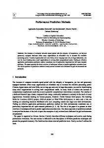
model of the communication cost for cubic domains is complex and the implementers of hypre have remarked that it would be unmanageably complicated for non-cubic domains. Further, Figure 1 indicates these parameters significantly impact performance: execution time varies by up to a factor of five under varying processor topologies for a fixed problem size. 2.2.2

High-Performance Linpack

HPL solves dense linear systems by performing an iterative LU decomposition followed by backward substitution [1]. The panel decomposition occurs recursively in a given iteration. A cyclic scheme distributes blocked data onto a two-dimensional grid of processors to ensure load balance and scalability. Table 3 shows the eight-dimensional input parameter space of our HPL experiments in which we hold the total matrix size (defined by N ) constant. N B is the matrix block size, which we vary between ten and eighty on BG/L and ten and a hundred on ALC and MCR. P and Q describe the processor topology in two dimensions (P ×Q = 512 on BG/L and 64 on ALC and MCR). BCAST specifies variants of broadcast algorithms with the first two parameters specifying increasing one ring virtual and modified topologies, the next two specifying corresponding two ring topologies, and the last two specifying long message variants. The panel and recursive factorization (P F ACT , RF ACT ) may each employ three variants: right-looking, left-looking, and Crout’s method. The number of sub-panels (NDIV) and number of columns in the recursive base case (NBMIN) are also tunable. Our HPL parameter space is large with over 900,000 points on BG/L. Figure 1 demonstrates HPL execution time varies significantly with data organization and processor topology. Although some guidance is available for parameter choices, it is generally in terms of probable impact and sampling is recommended. By using modeling, we can improve the value of that sampling. 2.3

Software Packages

We use R, a free software environment for statistical computing, to script and automate the statistical analyses described in Section 2.4 and Section 3.2. Within this environment, we use the Hmisc and Design packages implemented by Harrell [7]. We use the Stuttgart

180

80

160

70

140

50

Execution time (s)

Execution time (s)

60

40 30 20

120 100 80 60 40

10

20

0 0

100000

200000

300000

0

Working set size (Nx*Ny*Nz)

Experiments ordered by P, NB

Figure 1. 512-node BG/L performance of SMG2000 for varying workloads, processor topologies (L) and HPL for varying block sizes, processor topologies (R).

nz

nx

ny pz

py

px

0.4 0.6

tinit

0.8

tsolve

Clustering is a common statistical technique that classifies data elements based on a measure of similarity. A symmetric N ×N matrix S describes the similarity of N elements: S(i, j) quantifies the similarity between elements i and j. Hierarchical clustering iteratively identifies similar elements through the following algorithm:

tset

Hierarchical Clustering

1.0

2.4.1

0.2

Statistics

We illustrate statistical analyses for SMG2000 on BG/L based on data collected sparsely, uniformly at random from the parameter space. Similar techniques are applied to other applications and platforms. These techniques provide insight into the parameter space, revealing significant relationships between variables and characterizing observed trends.

Spearman ρ2

2.4

0.0

Neural Network Simulator (SNNS) to construct the networks described in Section 3.3. SNNS performs operations for learning and prediction for various network architectures [20].

Figure 2. Hierarchical clustering for SMG2000 on BG/L.

• Initialize: Create N unique single-element clusters. • Merge: Combine most similar pair of clusters into one cluster. • Iterate: Repeat merge until one N -element cluster is obtained.

The similarity between two clusters A and B is the maximum similarity between elements of each cluster: S(A, B) = max{S(x, y) : x∈A, y∈B}. Correlation is our measure of similarity between two parameters. Thus, hierarchical clustering provides insight into the relationships between parameters through their correlations. Figure 2 plots the clustered predictors and responses for SMG2000. The correlation between the processor counts in three dimensions is an artifact of our constraint: Px × Py × Pz = 512. The correlation between working set sizes in three dimensions results from constraining the total problem size to fit in memory. Lastly, the correlation between components of execution time are significant; solve time is highly correlated with initialization and setup time. Hierarchical clustering can also guide regression modeling to ensure redundant predictors are not included in the model when there are many potential predictors. If multiple predictors are highly correlated and classified into the same cluster, a single representative predictor can often capture its cluster’s impact on the response. Similarly, if multiple responses are highly correlated, a single model may be constructed for a representative response since correlated responses will likely trend with the modeled response.

For SMG2000, the correlation between execution time components leads us to a model that only predicts solve time since it should also be representative of the other smaller execution time components. Pruning the number of predictors is important as it controls the size of the model, not only by controlling the number of predictors but also controlling the number of potential interactions between predictors. A number of studies in which models are validated on independent data sets have shown a fitted regression model is likely reliable (no over-fitting) when the number of samples n is 20 times the number of predictors [7]. Thus, smaller models reduce the number of samples required to mitigate over-fitting risk. 2.4.2

Association Analysis

We can also examine each predictor’s association with the response to gain further insight into their importance. Scatterplots qualitatively illustrate the association between predictors and the response, revealing potential non-monotonicity or non-linearity. These plots may quickly reveal significant predictors by demonstrating, for example, a clear monotonic relationship with the response. Conversely, plots exhibiting low response variation despite a changing predictor value might suggest predictor insignificance. Thus, scatterplots allow the modeler to quickly understand the parameter space at a high level.

3.

Modeling Techniques

Given a set of sparsely collected performance measurements, we construct predictive models using two techniques in generalized non-linear regression: piecewise polynomial regression and neural networks. Piecewise polynomial regression emphasizes domainspecific knowledge and statistical analysis in model construction while neural networks emphasize usability and automation. 3.1

Figure 4. Correlation analysis for SMG2000 on BG/L.

Figure 3 plots predictor-response associations dividing the predictor domain into intervals. The average response of each interval’s samples are plotted. For example, Nz has a value between 102 and 506 for 248 of 1,000 samples. The average solve time for these samples is 35.0 seconds. These plots illustrate monotonic relationships for the working set sizes in the y- and z-dimensions, but non-monotonic relationships for the processor counts in three dimensions. The plot for Nz suggests a particularly strong relationship between Nz and the execution time. This is consistent with our domain-specific understanding of the semicoarsening multigrid algorithm. SMG2000 coarsens only in the z-dimension and the costly iterative relaxation in this dimension depends on Nz , requiring communication between x-y planes. 2.4.3

Correlation Analysis

Although we qualitatively observe marginal relationships between each predictor and the response in the previous scatterplots, we have not quantified the strength of these relationships. The relative strength of scatterplot relationships is quantified by the correlation between variables. Pearson’s correlation coefficient for random variables X,Y is a function of expectations µx ,µy and standard deviations σx ,σy for n observations. Non-parametric statistics are more robust if the distribution of X, Y are unknown. We prefer the Spearman Rank correlation coefficient of Equation (1) that can quantify association independently of variable distribution. The computationally efficient approximation only requires di , the difference in ordinal rank of Xi in X and Yi in Y . n X Xi Yi d2i ≈ 1 − 6 ” 1/2 P n(n2 − 1) n 2 2 i=1 i=1 Xi j=1 Yj

Pn

ρsp = “ Pn

i=1

(1)

Figure 4 ranks predictors by their correlation coefficients to support assessments of their relative significance. Predictors with higher rankings will require more flexible non-linear transformations than those with lower rankings since any lack of fit for these highly ranked predictors will negatively impact overall model accuracy more significantly. As in the association analysis, we find Nz and Ny most highly correlated with solve time, observing correlation coefficients of 0.145 and 0.031, respectively. All other predictors are less strongly correlated, if at all, with performance.

Configuration Sampling

The prohibitively high costs of exhaustive performance measurements for each point in our parameter space motivate a sparse sampling from the space. The performance of these samples, representing a particular application input set, is collected to produce observations. The approach to sampling for observations significantly impacts the accuracy of predictive models as exhaustive measurement becomes inefficient and impractical. Piecewise polynomial regression and artificial neural networks each utilize particular sampling techniques to improve accuracy. Sampling Uniform at Random: We propose sampling points uniformly at random (UAR) from the parameter space. This approach provides observations from the full range of parameter values and enables identification of trends and trade-offs between parameters. We may consider an arbitrarily large number of possible values for any given parameter since we decouple the number of measurements from the parameter space size via random sampling. Furthermore, samples obtained uniformly provide unbiased observations such that the parameter space is well represented in data used to construct regression models or neural networks. Stratification: Regression and neural networks optimize coefficients or edge weights to minimize sum of square errors. However, this objective may give undue emphasis to samples with larger performance measurements since their modeled absolute errors are likely larger. Conversely, samples with small performance values may be less influential in model construction due to their small absolute errors. Stratification mitigates this bias by giving additional weight to samples with small performance values, replicating each sample by a factor proportional to the inverse of its observed response. Targeting samples with small performance values that have large relative but small absolute errors, this technique reduces the divergence in relative error across the parameter space. Regional Sampling: A variant on UAR sampling, regional sampling formulates per-query regression models using only points most similar to the query. We quantify similarity by the Euclidean distance between vectors of normalized and weighted parameter values. Specifically, values are normalized by subtracting the mean and dividing by the standard deviation. They are also weighted according to their correlation with performance. This weighting emphasizes parameters that significantly impact performance in the distance calculation. Regional sampling incurs additional modeling costs as Euclidean distances are computed and regression models are formulated for each query. This technique is combined with regression for all data sets except those for HPL data collected on BG/L and MCR. In these two sets, sampling uniformly at random and stratification are sufficient to formulate effective models. 3.2 3.2.1

Regression Formulation

We consider a general class of regression models in which a response is modeled as a weighted sum of predictor variables plus random noise. For a space of interest, suppose we have a subset of n observations for which values of the response and predictor variables are known. Let y = y1 , . . . , yn denote the vector of observed responses. For a particular point i in this space, let yi denote its response and xi = xi,1 , . . . , xi,p denote its p predic-

Working Set Size

Processor Distribution N

nx

[ 10, 24) [ 24, 51) [ 51,127) [127,501]

● ● ● ●

250 252 248 250

[0,2) [2,4) [4,6) [6,9]

254 250 250 246

[0,2) 2 [3,6) [6,9]

257 243 252 248

[0,2) [2,4) [4,6) [6,9]

ny

● ● ● ●

339 270 201 190

py

[ 10, 24) [ 24, 51) [ 51,118) [118,505]

● ● ● ●

nz

[ 10, 23) [ 23, 45) [ 45,102) [102,506]

N

px

348 159 337 156

● ● ● ●

pz ● ● ● ●

Overall

● ● ● ●

329 268 222 181

Overall 1000

●

25

30

1000

●

35

24

tsolve

25

26

27

28

29

tsolve

N=1000

N=1000

Figure 3. Association plots for SMG2000 on BG/L. tors. These variables are constant for a given point in the space. Let β = β0 , . . . , βp denote the corresponding set of regression coefficients used in describing the response as a linear function of predictors plus a random error ei as in Equation (2). The ei are assumed independent random variables with zero mean and constant variance: E(ei ) = 0 and V ar(ei ) = σ 2 . f (yi ) = β·g(xi ) + ei = β0 +

p X

βj gj (xij ) + ei

(2)

j=1

Transformations f and g = g1 , . . . , gp may be applied to the response and predictors, respectively, to improve model fit by stabilizing a non-constant error variance or accounting for non-linear predictor-response relationships. 3.2.2

Interaction and Non-Linearity

In some cases, the effect of two predictors xi,1 and xi,2 on the response cannot be separated; the effect of xi,1 on yi depends on the value of xi,2 and vice versa. The interaction between two predictors may be modeled by constructing a third predictor xi,3 = xi,1 xi,2 to obtain yi = β0 + β1 xi,1 + β2 xi,2 + β3 xi,1 xi,2 + ei An assumption of linearity is often too restrictive and several techniques for capturing non-linearity may be applied. The most simple of these techniques is a polynomial transformation on predictors suspected of having a non-linear correlation with the response. However, polynomials have undesirable peaks and valleys. Furthermore, a good fit in one region of the predictor’s values may unduly impact the fit in another region of values. For these reasons, splines are a more effective technique for modeling non-linearity. Spline functions are piecewise polynomials. The predictor domain is divided into intervals divided by knots with different continuous polynomials fit to each interval. The number of knots can vary but more knots generally leads to better fits. Cubic splines are particularly effective as they may be smoothed at the knots by forc-

ing first and second derivatives to agree [7]. We perform regression on restricted cubic splines, constructing models with linear tails and interior piecewise cubic polynomials. The choice and position of knots are variable parameters when specifying non-linearity with splines. Placing knots at fixed quantiles of a predictor’s distribution is a good approach in most datasets, ensuring a sufficient number of points in each interval [17]. In practice, five knots or fewer are generally sufficient for restricted cubic splines. Fewer knots may be required for small data sets. As the number of knots increases, flexibility improves at the risk of over-fitting the data. In many cases, four knots offer an adequate fit of the model and is a good compromise between flexibility and loss of precision from over-fitting [7]. For example, regression models for SMG2000 predict solve time from processor topology and working set size. Predictor interactions are specified with domain-specific knowledge. We expect interaction between Pz and Nz because processor count in the z-dimension may impact solve time differently for different working set sizes in the z-dimension. Similarly, we specify interactions between predictors in different dimensions (e.g., Py and Pz ) to capture inter-dimensional trade-offs necessary to meet constraints on the total processor count and the total problem size. Restricted cubic splines are specified using four knots for all predictors except Nz , which uses five knots due to its significance observed in preliminary statistical analyses. 3.2.3

Construction

The method of least squares identifies coefficients that minimize the sum of squared deviations in Equation (3) for a given specification of predictors, interaction, and non-linearity and a given set of observations. This minimization requires solving a system of p + 1 partial derivatives of E with respect to βj , j ∈ [0, p]. Least squares often marks the midpoint in the model design process. Additional analysis of the new formulated model may examine fit to the ob-

Figure 5. Feedforward neural network with one hidden layer (p=3 and H=4).

Figure 6. Sigmoid function. tunable parameter in network construction. Let w = w1 , . . . , wH denote edge weights communicating outputs from the hidden layer b = b1 , . . . , bH into the output layer. Furthermore, assume all non-input neurons implement the same activation function f . For a three-layer network, the final output yˆ is computed by Equation (6) where bj is expanded with Equation (5) that computes hidden layer output from network inputs x.

served data and statistical significance of predictors and terms comprising the model [12].

E(β0 , . . . , βp ) =

n X

yi − β 0 −

i=1

3.2.4

p X

!2 βj xij

(3)

j=1

Prediction yˆ = f (w·b) = f

Once regression coefficients are determined by least squares, evaluating Equation (2) for a given xi will give the expectation of yi and, equivalently, the estimate yˆi for yi in Equation (4). This result follows from the additive property of expectations, the constant expectation of a constant and the zero mean of random errors. # " p p X X ˆ ˜ ˆ ˜ βj xij yˆi = E yi = E β0 + βj xij + E ei = β0 + j=1

j=1

3.3 3.3.1

Artificial Neural Networks Formulation

Artificial Neural Networks (ANNs) are a class of machine learning models that map predictors to a response using a network of neurons, simple processing elements, connected by weighted edges. As in regression, consider an observed sample with known predictor and response vectors x and y. For a particular neuron j in the network, let bj denote its output and a = a1 , . . . , ap denote its p potentially transformed versions of x. If the inputs arrive via edges with weights vj = vj,1 , . . . , vj,p , the neuron computes its output as a weighted sum of inputs in Equation (5). An activation function f may transform the weighted sum to increase the set of mappings the network is able to represent.

bj = f (vj ·a) = f

p X

! vj,k ak

(5)

k=1

Multi-layered neural networks increase this framework’s representational power and can approximate any function to arbitrary precision [15]. Neurons in the input layer implement the identity activation function, passing predictor values to the hidden layers. These layers pass inputs through successive linear combinations, transformations before computing the final network output. Consider the three-layer network illustrated in Figure 5 that implements a fully connected feedforward architecture in which every neuron in a layer is connected to all neurons in the previous layer. Suppose the input layer contains p neurons corresponding to the p predictors and the hidden layer contains H neurons where H is a

H X j=1

3.3.2

(4)

! wj bj

=f

H X j=1

wj f

p X

!! vj,k xk

k=1

Interaction and Non-Linearity

Predictor impact on the response is determined by the edge weights connecting the nodes. Since Equation (6) does not consider products of terms, the network does not provide a mechanism for automatically identifying predictor interaction in which the effect of two or more predictors on the response cannot be separated. Although such interactions may be captured by specifying inputs as products of predictors (e.g. x3 = x1 x2 in Figure 5), our results suggest the sigmoid function sufficiently captures interactions, eliminating the need for domain-specific knowledge. Non-linearity is modeled by activation functions f at each neuron. For our automated approach to neural network construction, we assume input neurons implement the identify function f (x) = x and non-input neurons implement the sigmoid function f (x) = 1/(1+e−x ) of Figure 6. More generally, non-input activation functions should be non-linear, monotonic, and differentiable [15]. 3.3.3

Construction

The edge weights of neural networks must be updated to capture trends in observed samples. Edge weights are initialized near zero and backpropagation updates weights by gradient descent to minimize squared error E between the n network predictions and observed sample responses. In particular, the weight Wi,j of an edge between neurons i and j is iteratively updated by Equation (8) where η specifies learning rate. A momentum term may help backpropagation avoid local minima by adding a fraction α of the weight changes from the previous iteration ∆Wi,j (t − 1). Momentum accelerates gradient descent in low-gradient regions and damps oscillations in highly non-linear regions. This work uses a three-layer neural network with a 16-neuron hidden layer, initial weights drawn uniformly from [-0.01,+0.01]. Values for the learning rate and momentum term are determined automatically with an adaptive variant of backpropagation, resilient backpropagation [16]. These values work well in practice for a few different parameter space studies and tuning the network design was unnecessary.

(6)

3.4.1 E(W )

=

n X (yi − yˆi )2

(7)

i=1

W (t)i,j

=

Wi,j −

! ∂E + α∆Wi,j (t − 1) η ∂Wi,j

(8)

Artificial neural networks may mitigate over-fitting risk by halting gradient descent before it converges to edge weights that minimize error on the training samples [5, 15]. In particular, a portion of the training samples is designated the early stopping set and gradient descent for the remaining samples is halted when the network’s squared error converges for the early stopping set. Early stopping reduces risk of over-fitting to observed data since the halting criterion does not utilize the full set of sampled observations. Since the early stopping set is used only for the halting criterion and not used in gradient descent, this technique reduces the number of samples available for network training. Cross validation mitigates the impact of fewer samples by constructing multiple neural networks trained on different subsets of the data. This technique divides the training samples into multiple, equally sized subsets. Consider cross validation with 10 subsets each containing 10% of the samples. A network is trained on subsets 1-8 using subset 9 for early stopping and subset 10 for validation. A second network is trained on subsets 2-9 using subset 10 for early stopping and subset 1 for validation. Repeating this process, cross validation will thus create ten networks. The ten corresponding outputs are averaged to produce the ensemble network output. Although only 80% of samples are used to train any one model, all samples are used to train eight of ten models in the ensemble. Thus, the ensemble performs similarly to a model using the full samples, yet reserves samples for the early stopping set. In practice, an average of multiple models may mitigate the risk of particularly high error variance in any one model. The mean and deviations of the ten model errors observed for the validation subsets are used to estimate ensemble error. Cross validation reduces error variance and improves estimates of ensemble accuracy at the expense of additional computation to train multiple models. 3.3.4

Prediction

Once backpropagation by gradient descent has converged, the network performs predictions by applying inputs to the network, evaluating Equation (6) for each prediction. Thus, a multi-layer neural network models the predictor-response relationship with nested non-linear weighted sums. Additional hidden layers can further increase the representational power by increasing the nesting depth. 3.4

Theoretical Comparison

Piecewise polynomial regression and neural networks both model a response as non-linear weighted sums of predictors. In both techniques, the weights are determined to minimize model error based on sampled observations of predictor-response tuples. However, the techniques differ in their approaches to specifying model form and optimizing model weights, illustrating more general differences between statistical inference and machine learning. Model formulation for statistical inference is often guided by domain-specific knowledge and statistical analyses of incompletely observed data. In contrast, machine learning use the same observed data to construct a model, minimizing criteria of fit by heuristic search in attempts to automate steps in model formulation. A theoretical comparison between piecewise polynomial regression and neural networks illustrates trade-offs between statistical understanding and automation while revealing differences in computational efficiency.

Statistics and Automation

Piecewise polynomial regression relies on clustering, association, and correlation analyses to identify relevant predictors and interesting predictor-response relationships. These statistical techniques are combined with domain-specific knowledge to guide the specification of predictor interactions and non-linearities. Additional statistical tests may be necessary after model construction to ensure model fit and a lack of systematic bias. Although these analyses require a modest background in statistics, they lead to a better understanding of the parameter space. In contrast, neural networks offer an automated approach by providing a flexible model specification (i.e., nested weighted sums on sigmoid activation functions). This framework assumes all predictors are relevant prior to network construction, relying on machine learning to assign appropriate weights to predictors based on their contributions to the sum of square errors. An untrained network has the potential to specify many functional forms of predictor-response relationships and the ultimate form is obtained automatically given training data. Thus, neural networks offer greater usability at the expense of greater statistical understanding of the parameter space. Regression is a relatively transparent technique, exposing predictor interaction and non-linearity to the user. The functional form of the predictor-response relationship is based on statistical analysis and domain-specific knowledge, ensuring consistency between the model and user intuition. Neural networks are often treated as an automated black box consuming predictor values to generate response predictions. The underlying mechanism generating these predictions is less open to interpretation since it incorporates no domain knowledge and predictor-response relationships may be obscured by the nesting of non-linear sums. Thus, regression offers greater transparency at the cost of greater statistical analysis while neural networks offer greater automation with some cost in statistical insight. 3.4.2

Computational Efficiency

Both piecewise polynomial regression and neural networks determine weights to minimize sum of square errors. After linearizing transformations, regression expresses this optimization as linear least squares that explicitly solves a linear system using a QR or Cholesky decomposition. In contrast, neural network edge weights are iteratively refined to reduce error, evaluating the network in every iteration of gradient descent to approximate a solution to least squares. The time to convergence in learning is usually larger than that required to solve least squares in regression numerically, especially if the predictor count is small. Given transformed predictors, regression computes the response as the weighted sum in Equation (4). Neural networks compute a nested weighted sum of predictors with multiple transformations. Specifically, Equation (6) expresses the output of a network with one hidden layer as a non-linear function (sigmoid at output layer) of a weighted sum (input to output layer) of non-linear functions (sigmoid at hidden layer) of a weighted sum of inputs (input to hidden layer). Thus, piecewise polynomial regression is more computationally efficient at the cost of additional statistical analysis before and after model formulation. Neural networks are less efficient, but rely less on domain knowledge and intuition. Assuming equally accurate predictions, the two techniques represent a choice between statistical effort and automation.

4.

Model Evaluation

4.1

Prediction Accuracy

Figure 7 presents boxplots of the error distributions for performance predictions of 100 validation points sampled UAR from the parameter space. The error is expressed as |obs−pred|/pred. Box-

plots are graphical displays of data that measure location (median) and dispersion (interquartile range), identify possible outliers, and indicate the symmetry or skewness of the distribution. Boxplots are constructed by 1. horizontal lines at the median and at the upper, lower quartiles 2. vertical lines drawn up/down from the upper/lower quartile to the most extreme data point within 1.5 IQR of the upper/lower quartile with horizontal lines at the end of the vertical lines 1 3. circles beyond the ends of vertical lines to denote outliers Figure 7(L) indicates piecewise polynomial regression achieves median errors between 2.2 percent (hpl-mcr) and 9.4 percent (smgmcr). 75 percent of predictions achieve error rates of 16 percent or less. HPL predictions (median errors of 2.2 to 5.2 percent) are more accurate than SMG predictions on the same platform (median errors of 6.3 to 9.4 percent) as regression leverages additional algorithmic predictors. Outlier error not shown includes three predictions for SMG on ALC with errors of 56.7, 62.6, and 98.0 percent. Figure 7(R) considers neural networks for the same predictions. Median error rates range from 3.6 (smg-alc) to 10.5 (hpl-alc) percent. Predictions are equally accurate for both applications with at most a 1 percent difference in median error between SMG and HPL predictions on the same platform. 75 percent of predictions achieve median error rates of 16.2 percent or less. Outlier error not shown includes two predictions for HPL with errors of 68.5 and 82.3 percent. Overall, regression and neural networks predict with similar median and outlier error rates. Examining the interquartile range, however, we observe a greater spread in SMG regression error relative to the spread in SMG network error. In particular, the difference between the 1st and 3rd quartile varies from 10.0 to 11.7 percent in SMG regression compared to a spread of 4.6 to 11.1 percent for SMG networks. Similarly, regression predictions tend to extend further from the 3rd quartile as illustrated by longer vertical lines above the boxes. We observe the opposite interquartile trends for HPL. The HPL regression is 4.5 to 12.0 percent compared to a spread of 9.6 to 11.7 percent in networks. This reversal for HPL regression is attributed to particularly low spread in regression error on ALC and MCR. These platforms are notable for their high system noise relative to the effectively noise-less BG/L. 4.2

Sampling Sensitivity

In addition to considering prediction accuracy with 600 samples, we assess median error sensitivity to varying sample sizes. The BG/L HPL data of Figure 8(L) demonstrates accuracy benefits from additional samples with median errors falling from 7.6 to 6.5 percent and from 8.4 to 4.8 for regression and neural networks, respectively. Similar trends are observed for SMG2000 on MCR. In contrast, BG/L SMG2000 data of Figure 8(R) illustrates significant improvements for regression (from 11.9 to 7.5 percent) and relatively flat trends for neural networks (from 5.9 to 5.5 percent). To further illustrate the difficulty of identifying an optimal sample size, we observe flat trends for HPL on MCR in Figure 9(L) and non-monotonic trends for SMG2000 on MCR in Figure 9(R). In the latter case, we observe improving regression accuracy (from 9.6 to 8.0 percent) and network accuracy (from 8.5 to 7.3 percent) as additional samples are used in model construction. However, we also observe spikes in error rates at 400 samples for regression and 700 samples for both techniques as we approach the lower error rates of 1,000 samples. These trends illustrate the difficulty of identifying, a priori, an optimal sample size. Better selection of sample sizes is potentially future work. 1 IQR:

interquartile range is the difference between first and third quartile.

5.

Related Work

Although regression and neural networks have been separately applied to predict application and microarchitecture performance, we present a comparison of these techniques and highlight their relative strengths and weaknesses. These techniques apply inference and learning for empirical performance modeling. We contrast our approaches with previous work in parameter space analysis and performance modeling. 5.1

Regression and Neural Networks

Lee and Brooks apply piecewise polynomial regression to a large uniprocessor design space of nearly one billion points to perform accurate predictions of performance and power [13, 12]. Ipek, et al., predict performance of memory, core, and CMP design spaces with artificial neural networks [9]. While Ipek, et al. also apply neural networks to predict the performance of SMG2000 [8], they do not consider statistical techniques for preliminary data analysis and do not consider piecewise polynomial regression. In contrast, we analyze regression and neural networks in both theoretical and experimental comparisons. 5.2

Statistical Significance Ranking

Joseph, et al., derive performance models using stepwise regression, an automatic iterative approach for adding and dropping predictors from a model depending on measures of significance [10]. Although commonly used, stepwise regression has several significant biases cited by Harrell [7]. In contrast, we use domain-specific knowledge of microarchitectural design to specify non-linear effects and interaction between predictors. Furthermore, the authors consider only two values for each predictor and do not predict performance, using the models only for significance testing. Yi, et al., identify statistically significant processor parameters using Plackett-Burman design matrices [19]. Given these critical parameters, they suggest fixing all non-critical parameters to reasonable constants and gathering more extensive observations by sweeping a range of values for the critical parameters. We use various statistical techniques to identify significant parameters, but instead of gathering further observations, we rely on regression models based on these parameters to explore the parameter space. Furthermore, Placket-Burman specifies only bounds on parameter values while the techniques we present are applicable to measurements at finer parameter resolutions. 5.3

Models for Parallel Applications

Marin and Mellor-Crummey semi-automatically measure and model program characteristics, using properties of the architecture, properties of the binary, and application inputs to predict application behavior [14] . Their toolkit predefines a set of functions and the user may add customized functions to this library if needed. In contrast to our work, the authors vary the input size in only dimension and their models cannot account for some important architectural parameters (e.g., cache associativity in their memory reuse modeling). Carrington, et al., develop a framework for predicting scientific computing performance and demonstrate its application for HPL and an ocean modeling simulation [3]. Their automated approach relies on a convolution method that maps an application signature onto a machine profile. Simple benchmark probes create machine profiles and a separate tool generates application signatures. Extending the convolution method enables models of full-scale HPC applications [4]. They must gather a trace for each point in the parameter space. Depending on trace sampling rates, their predictions achieve error rates between 4.6 percent and 8.4 percent. Full traces obviously perform best, but such trace generation can slow application execution by almost three orders of magnitude.

Figure 7. Boxplots of the performance error distributions obtained via regression (L) and neural networks (R).

Figure 8. Sensitivity to sample size for BlueGene/L

Figure 9. Sensitivity to sample size for MCR

Kerbyson, et al., present an accurate, predictive analytical model that encompasses the performance and scaling characteristics of SAGE, a multidimensional hydrodynamics code with adaptive mesh refinement [11]. Inputs to their parametric model come from machine performance information, such as latency and bandwidth, along with application characteristics, such as problem size and decomposition. They validate model predictive accuracy against measurements on two large-scale ASCI systems. In addition to predicting performance, their model can yield insight into performance bottlenecks, but the application-centric approach requires static code analysis and a separate, detailed model must be developed for each target application. Yang, et al., develop cross-platform performance translation based on relative performance between target platforms without program modeling, code analysis, or architectural simulation [18]. As in our work, their method targets performance prediction for resource usage estimation. They observe relative performance through partial execution of two ASCI Purple applications. The approach works well for iterative parallel codes that behave predictably (achieving prediction errors of 2 percent or lower) and enjoys low overhead costs. Prediction error varies from 5 to 37 percent for applications with variable overhead per time step. Likewise, reusing partial execution results for different problem sizes and degrees of parallelization renders their model less accurate.

6.

Conclusion

We present a series of robust techniques for understanding large application parameter spaces and constructing predictive models for these spaces. In particular, we illustrate the application of statistical techniques, including clustering, association, and correlation analysis, for identifying significant contributions to application performance. We construct effective piecewise polynomial regression models and artificial neural networks that predict application performance as a function of its input parameters. Median error rates range from 2.2 to 10.5 percent across both techniques. A comparative analysis of regression and neural networks illustrate trade-offs between techniques. Regression offers greater transparency and statistical understanding while neural networks offer greater usability and automation. As both techniques offer comparable accuracy, the appropriate technique depends on the needs of the modeler. Regression and neural networks represent two extrema in a continuum that trades statistical rigor with automation. Future work may explore intermediate techniques such as automating the statistical techniques required for regression with heuristics. Similarly neural networks may leverage statistical analyses to customize activation functions or neural network weights. Acknowledgements Part of this work was performed under the auspices of the U.S. Department of Energy by University of California Lawrence Livermore National Laboratory under contract No. W-7405-Eng-48 (UCRL-CONF-227097). This work is also supported by NSF grants CCF-0048313 and CCF-0444413 in addition to support from Intel and IBM. Any opinions, findings, and conclusions or recommendations expressed in this material are those of the author(s) and do not necessarily reflect the views of the U.S. Department of Energy, University of California, National Science Foundation, Intel or IBM.

References [1] A.Petitet, R.Whaley, J.Dongarra, and A.Cleary. HPL - A portable implementation of the high-performance LINPACK benchmark for distributed-memory computers. www.netlib.org/benchmark/hpl.

[2] P. N. Brown, R. D. Falgout, and J. E. Jones. Semicoarsening multigrid on distributed memory machines. SIAM Journal on Scientific Computing, 21(5), 2000. [3] L. Carrington, A. Snavely, X. Gao, and N. Wolter. A performance prediction framework for scientific applications. In International Conference on Computational Science Workshop on Performance Modeling and Analysis (PMA03), June 2003. [4] L. Carrington, N. Wolter, A. Snavely, and C. Lee. Applying an automatic framework to produce accurate blind performance predictions of full-scale hpc applications. In Department of Defense Users Group Conference, June 2004. [5] R. Caruana, S. Lawrence, and C. Giles. Overfitting in neural nets: backpropagation, conjugate gradient, and early stopping. In Neural Information Processing Systems (NIPS), November 2002. [6] R. Falgout and U. Yang. Hypre: A library of high performance preconditioners. Springer LNCS, 2331, 2002. [7] F. Harrell. Regression modeling strategies. Springer, 2001. [8] E. `Ipek, B. de Supinski, M. Schulz, and S. McKee. An approach to performance prediction for parallel applications. Euro-Par, Springer LNCS, 3648, 2005. ` [9] E. Ipek, S. McKee, B. de Supinski, M. Schulz, and R. Caruana. Efficiently exploring architectural design spaces via predictive modeling. In Architectural Support for Programming Languages and Operating Systems (ASPLOS XII), October 2006. [10] P. Joseph, K. Vaswani, and M. J. Thazhuthaveetil. Construction and use of linear regression models for processor performance analysis. In International Symposium on High Performance Computer Architecture (HPCA-12), February 2006. [11] D. Kerbyson, H. Alme, A. Hoisie, F. Petrini, H. Wasserman, and M. Gittings. Predictive performance and scalability modeling of a large-scale application. In IEEE/ACM Supercomputing, November 2001. [12] B. Lee and D. Brooks. Accurate and efficient regression modeling for microarchitectural performance and power prediction. In Architectural Support for Programming Languages and Operating Systems (ASPLOS XII), October 2006. [13] B. Lee and D. Brooks. Illustrative design space studies with microarchitectural regression models. In International Symposium on High-Performance Computer Architecture (HPCA-13), February 2007. [14] G. Marin and J. Mellor-Crummey. Cross-architecture performance predictions for scientific applications using parameterized models. In International Conference on Measurement and Modeling of Computer Systems (Sigmetrics), June 2004. [15] T. Mitchell. Machine Learning. WCB/McGraw Hill, 1997. [16] M. Riedmiller and H. Braun. A direct adaptive method for faster backpropagation learning: The RPROP algorithm. In IEEE International Conference on Neural Networks, May 1993. [17] C. Stone. Comment: Generalized additive models. Statistical Science, 1, 1986. [18] T. Yang, X. Ma, and F. Mueller. Cross-platform performance prediction of parallel applications using partial execution. In IEEE/ACM Supercomputing, November 2005. [19] J. Yi, D. Lilja, and D. Hawkins. Improving computer architecture simulation methodology by adding statistical rigor. IEEE Computer, 54(11), 2005. [20] A. Zell and et. al. Snns: Stuttgart neural network simulator, user manual, version 4.2. In User Manual, Version 4.2, University of Stuttgart.