SANDIA REPORT SAND96-2000 • UC-405 Unlimited Release Printed August 1996
MIG 0.0 Model Interface Guidelines: Rules to Accelerate Installation of Numerical Models Into any Compliant Parent Code.
R. M. Brannon, M. K. Wong Prepared by Sandia National Laboratories Albuquerque, New Mexico 87185 and Livermore, California 94550 for the United States Department of Energy under Contract DE-AC04-94AL85000 Approved for public release; distribution is unlimited.
Issued by Sandia National Laboratories, operated for the United States Department of Energy by Sandia Corporation. NOTICE: This report was prepared as an account of work sponsored by an agency of the United States Government. Neither the United States Government nor any agency thereof, nor any of their employees, nor any of their contractors, subcontractors, or their employees, makes any warranty, express or implied, or assumes any legal liability or responsibility for the accuracy, completeness, or usefulness of any information apparatus, product, or process disclosed, or represents that its use would not infringe privately owned rights. Reference herein to any specific commercial product, process, or service by the trade name, trademark, manufacturer, or otherwise, does not necessarily constitute or imply its endorsement, recommendation, or favoring by the United States Government, any agency thereof or any of their contractors or subcontractors. The views and opinions expressed herein do not necessarily state or reflect those of the United States Government, any agency thereof or any of their contractors.
Printed in the United States of America This report has been reproduced directly from the best available copy. Available to DOE and DOE contractors from Office of Scientific and Technical Information PO Box 62 Oak Ridge, TN 37831 Prices available from (615) 576-8401, FTS 626-8401 Available to the public from National Technical Information Service US Department of Commerce 5285 Port Royal Rd Springfield, VA 22161 NTIS price codes Printed copy: A08 Microfiche copy: A01
SAND96-2000 Unlimited Release Printed August 1996
Distribution Category UC-405
MIG Version 0.0 Model Interface Guidelines: Rules to Accelerate Installation of Numerical Models Into Any Compliant Parent Code Rebecca M. Brannon† and Michael K. Wong‡ †Computational
Physics and Mechanics Physics Research and Development Sandia National Laboratories Albuquerque, NM 87185-0820
‡Computational
Abstract A set of model interface guidelines, called MIG, is presented as a means by which any compliant numerical material model can be rapidly installed into any parent code without having to modify the model subroutines. Here, “model” usually means a material model such as one that computes stress as a function of strain, though the term may be extended to any numerical operation. “Parent code” means a hydrocode, finite element code, etc. which uses the model and enforces, say, the fundamental laws of motion and thermodynamics. MIG requires the model developer (who creates the model package) to specify model needs in a standardized but flexible way. MIG includes a dictionary of technical terms that allows developers and parent code architects to share a common vocabulary when specifying field variables. For portability, database management is the responsibility of the parent code. Input/output occurs via structured calling arguments. As much model information as possible (such as the lists of required inputs, as well as lists of precharacterized material data and special needs) is supplied by the model developer in an ASCII text file. Every MIG-compliant model also has three required subroutines to check data, to request extra field variables, and to perform model physics. To date, the MIG scheme has proven flexible in beta installations of a simple yield model, plus a more complicated viscodamage yield model, three electromechanical models, and a complicated anisotropic microcrack constitutive model. The MIG yield model has been successfully installed using identical subroutines in three vectorized parent codes and one parallel C++ code, all predicting comparable results. By maintaining one model for many codes, MIG facilitates code-to-code comparisons and reduces duplication of effort, thereby reducing the cost of installing and sharing models in diverse new codes.
Acknowledgment By providing numerous useful suggestions, the following people (listed in order from earliest to most recent involvement) have been instrumental in the development of MIG. Their time, patience, and encouragement is greatly appreciated. Paul Yarrington and Mike McGlaun: provided general comments and management support. Steve Attaway: helped shape the appearance and syntax of the ASCII data file. Pointed out the distinction between model and data units. Stressed the importance of data ordering in drivers. Paul Taylor: provided his version of the Steinberg-Guinan-Lund model as the first model to be “migized”. Acted as the first MIG developer to build a new model (Bammann-Chiesa) using MIG. Gene Hertel: provided comments and support. Was first to read and follow written instructions for installation of a MIG model into CTH. Gordy Johnson and Bob Stryk: provided much useful feedback and beta comments, especially improving the migtionary. Were first to install a MIG model (SGL) into a non-Sandia code (EPIC). Glenn Randers-Pehrson: meticulously read — and greatly improved — early drafts of the document. Pointed out issues regarding common block communication. Inspired developer’s code of honor. Was first to install a MIG model into Livermore-DYNA. Dave Benson: sparked interest in MIG within academia. Archie Farnsworth: acted as a developer retrofitting an existing model to MIG format; also developed MIG-compliant electromechanical models. Fred Norwood: offered many insightful editorial comments that greatly improved the version 0.0 guidelines.
ii
Contents Acknowledgment ....................................................................................................... ii Preface........................................................................................................................ vi Introduction................................................................................................................ 1 Scope.................................................................................................................... 2 How to use this document.................................................................................... 3 The Standard MIG model package ...................................................................... 5 Roles of the developer, architect, and installer .................................................... 7 The Model Developer ................................................................................................ 8 What constitutes a MIG model package? ............................................................ 8 ASCII data file ..................................................................................................... 9 Required routines ................................................................................................. 18 MIG utilities......................................................................................................... 27 Models with special needs ................................................................................... 28 Creating a MIG package step-by-step.................................................................. 29 Developer’s code of honor................................................................................... 30 The Parent Code Architect......................................................................................... 32 Automation .......................................................................................................... 33 Partial functionality.............................................................................................. 34 Sharing models between different parent codes .................................................. 34 ASCII data processing in general ........................................................................ 35 Required Routines................................................................................................ 35 Storage allocation in general................................................................................ 37 Interface drivers in general .................................................................................. 39 Processing migtionary terms................................................................................ 40 Summary .............................................................................................................. 41 The Model Installer.................................................................................................... 42 Model installation instructions for CTH .............................................................. 42 Model installation instructions for ALEGRA...................................................... 42 References.................................................................................................................. 43 APPENDIX A: MIG Primer ...................................................................................... A-1 Part 1: DEVELOPER’s Guide. ............................................................................ A-1 Part 2: ARCHITECT’s and INSTALLER’s Guide. ............................................ A-10 APPENDIX B: MIGTIONARY ................................................................................ B-1 Key to variable types ........................................................................................... B-3 The MIGtionary ................................................................................................... B-9 OPERATORS ...................................................................................................... B-38 APPENDIX C: Unit Keywords ................................................................................. C-1 APPENDIX D: Sample MIG package....................................................................... D-1 ASCII data file ..................................................................................................... D-1 Data Check Routine ............................................................................................. D-3 Extra Variable Routine ........................................................................................ D-6 Driver Routine ..................................................................................................... D-8 APPENDIX E: MIGCHK .......................................................................................... E-1 Getting started...................................................................................................... E-1
iii
Getting help.......................................................................................................... E-1 Using MIGCHK to create a model package ........................................................ E-2 STEP 1: Generate fill-in-the-blanks template for the ASCII data file................. E-3 STEP 2: Create the ASCII data file ..................................................................... E-7 STEP 3: Check and correct the ASCII data file................................................... E-8 STEP 4: Examine the “check” file output by migchk.......................................... E-9 STEP 5: Examine the “skeleton” file output by migchk...................................... E-11 STEP 6: Transform the skeletons into actual working subroutines..................... E-17 STEP 7: Deliver the completed MIG package to a model installer..................... E-21 Creating an unabridged migtionary ..................................................................... E-23 Creating an abridged migtionary ......................................................................... E-23 Adding terms to the migtionary ........................................................................... E-26 Checking an ASCII data file using an abridged migtionary ................................ E-26 Generating includes for rapid package installation.............................................. E-26 Testing the SGL model ........................................................................................ E-30 APPENDIX F: MIG-compliance of Particular Parent Codes.................................... F-1 ASCII data processing in CTH ............................................................................ F-1 ASCII data processing in ALEGRA .................................................................... F-2 Storage allocation in CTH ................................................................................... F-5 Storage allocation in ALEGRA ........................................................................... F-7 Interface driver for CTH ...................................................................................... F-8 Interface driver for ALEGRA.............................................................................. F-11 Processing migtionary terms in CTH (and migchk) ............................................ F-12 APPENDIX G: Development Log............................................................................. G-1 Unresolved Problems ........................................................................................... G-2 Resolved Problems............................................................................................... G-12 APPENDIX H: Viewgraphs ...................................................................................... H-1
iv
Figures Figure 1. Thumbnail sketch of the required data-check routine..............................
18
Figure 2. Thumbnail sketch of the required extra variable routine. ........................
21
Figure 3. Thumbnail sketch of the required model driver routine. .........................
24
Figure E-1.Taylor anvil benchmark geometry for the SGL model............................
E-30
Figure E-2.Yield stress as a function of time for both tracers from SGL benchmark calculations using parent codes (a) CTH and (b) ALEGRA. .................. E-31
Tables Table 1:
Ordered dimensions and associated units ................................................
v
14
Preface The model interface guidelines (MIG) originated on July 3, 1994, when members of the computational physics groups 1431 and 1432 (now 9231 and 9232) at Sandia National Laboratories posed the following challenge: Devise a way for our physics codes to all possess equivalent constitutive modeling capability, but do it in such a way that we need not maintain different versions of each material model for each parent code. The problem seemed simple enough, and we knew that such a capability would save much time in the long run. However, our physics codes were very different. The code with the most extensive selection of constitutive models was a vectorized finite-difference code written in FORTRAN. Another of our codes was built for world class parallel platforms, and was written in C++. Another possessed special data structures for the arbitrary LagrangeEulerian (ALE) method of solving the governing field equations. Clearly, to meet our challenge in a timely manner, we were going to have to avoid grandiose panaceas and concentrate only on primitives. What, we asked, was the absolute minimum to be done to use the same constitutive subroutines in all of our codes? At our first official meeting on July 19, 1994, we identified reasons why it was so hard to retrofit a material model from one code for use in another code. The obstacles were simple, but overwhelmingly abundant. For example, existing numerical models tended to contain common blocks and subroutine calls that depended on the parent code in which that model was originally installed. The scientist retrofitting the model for a new code would generally have to spend considerable time learning about the model physics in order to identify precisely what coding was science and what was merely parent code taskwork. Then the scientist would have to figure out how to replace the coding from the old parent code with equivalent coding for the new parent code. Similar delays resulted when the original model ran only on selected computer platforms, or only with specific compiler options, or only with a particular set of physical units. Another delay in retrofitting models from one code to another resulted from simple miscommunication (such as erroneous comment lines stating, for example, that a variable was a strain rate when in fact is was a strain increment). At our first meeting in the Summer of 1994, there was no dearth of obstacles to sharing models among our codes. Our charter was to devise workarounds (inelegant if necessary) for each impediment. The early result was what we then called SICOM (Standard Interface for COnstitutive Models). It was soon renamed MIG (Model Interface Guidelines) to emphasize that our concept wasn’t limited to only material models. Over the last two years, MIG has been continually modified to incorporate solutions to an incessant (but relenting) stream of snags. Fortunately, the rate of resolution of problems has exceeded the rate of creation of problems, and the current MIG has matured to a nearly stable state. We now offer this preliminary, still pliable, version to the scientific community specifically to solicit suggestions for improvement. Rebecca Brannon, Mike Wong, August 8, 1996
vi
[email protected] [email protected]
MIG 0.0
Introduction
MIG Version 0.0 Model Interface Guidelines: Rules to Accelerate Installation of Numerical Models Into Any Compliant Parent Code
Introduction This document is version “zero” of the Model Interface Guidelines, or “MIG” for short. Being neither software nor hardware, MIG is a set of standardizing rules that specify how developers can “package” fundamental model components (such as input/output lists, precharacterized model data, physics routines, model units, etc.) so that any MIG-compliant model may be rapidly installed into diverse parent codes* without having to modify the model subroutines. Advantages of such standards include: •Reduced model development time. The theorist may focus on properly capturing the model physics, spending less time on code-dependent taskwork such as establishing storage, reading inputs, etc. •Reduced installation time. By standardizing primitive model needs, less effort is required to install new material models into parent codes. MIG is designed so that all information needed to install a model may be found in the standardized package. The uniform structure of all standardized MIGmodels permits optional development of automated installation. •Model portability. Installation “hooks” (required, for example, to read material input data, reserve storage, etc.) can be added cleanly and automatically, thereby avoiding invasive installations which can hinder porting the model to different codes or computer platforms. •Model maintenance and code-to-code consistency. Model standards allow a single version of a model to be used in multiple codes, thus accelerating dissemination of model enhancements and guaranteeing fair code-to-code comparisons. Being “version zero,” this edition of the Model Interface Guidelines must be regarded as a preliminary or beta standard, subject to extensive revision and correction without notification and probably without support in later versions. Readers are strongly encouraged to offer suggestions and corrections during this development phase. Before doing so, however, please review Appendix G, which chronicles most of the resolved and unresolved problems addressed since the inception of these standards. * that is, programs (finite-element, finite-difference, particle, element-free, etc.) that have been suitably modified to accept MIG models.
1
Introduction
MIG 0.0
Scope In this document, a “model” is defined as a “black box” that requires a specific set of quantifiable inputs and provides a specific set of quantifiable outputs. This definition spans a purposely general range. A model could be a material plasticity rule that requires the stress and velocity gradient as input and supplies an updated yield stress as output. A model could be an electrochemical rule that requires magnetic flux and rate of reaction as inputs and supplies temperature as an output. A model could be a socioeconomic rule that requires the inflation rate as input and supplies an unemployment rate as output. A model could even be a more grandiose black box containing, say, an entire finite element code that requires element sizes as input and supplies convergence rates as output. In this early phase of the development of MIG, we have limited specific examples to material models of the sort commonly seen in large thermomechanical structural or physics codes, but the guidelines are designed to naturally accommodate other applications. Streamlining the process of model installation and maintenance is an ambitious charter for which MIG is only a first step. To skirt a spectrum of special or unpredictable code requirements, MIG standardizes only model primitives, that is, only tasks that all models generally share. For example, MIG specifies how the model developer (who knows the model physics and packages it in numerical form) must list user input requirements, unit dependencies, special storage requests, and many other fundamental model needs. MIG also specifies where (on an argument list) the model should supply promised model output. For the most part, MIG does not restrict what a model may request as input or supply as output. Nor does MIG dictate how the model computes its output. This is not to say that such guidelines wouldn’t be useful; they are simply not covered under MIG. The model developer only states (in a standardized way) what is needed from the parent code; actually acquiring and supplying these needs is the responsibility of the code architect who modifies a particular parent code to run MIG-compliant models. MIG standardizes the “hooks” extending from any MIG model, but not the way in which they are to be used. MIG does not standardize how the code architect must run a MIG model. Because MIG models only specify needs, the architect is free to satisfy these needs in any manner (most likely consistent with the way such needs are handled for the non-MIG models in a given code). Hence, the parent code architect may ensure that the user interface for MIG models looks and feels identical to the interface for all the non-MIG models already installed in the code.
2
MIG 0.0
Introduction
Because all MIG models are structured similarly, the code architect will probably begin to recognize repetitive tasks when installing models. For example, the architect may notice that the user input list is always in the same place for each MIG model and that these inputs are acquired from the code users via a parent code fragment that is similar in structure for all MIG models. The code architect initially creates these code fragments by hand (as for non-MIG models), but the constancy of MIG models may eventually prompt the architect to write utility scripts to generate the required code fragments for the simplest model primitives. One vision of the legacy of model guidelines is that a parent code’s useful installation scripts and instructions may slowly coalesce into a streamlined model installation process. Ideally, this process could be performed rapidly by any model installer who knows how to run the scripts but who need not be so intimately familiar with either the parent code or the model. MIG does not demand or guarantee the existence of time-saving installation procedures — MIG merely enables their eventual development at the discretion of each parent code’s architect.
How to use this document MIG’s beta testers (working with one or more of the production thermomechanics codes CTH [1], ALEGRA [2], EPIC [3], and LLNL-DYNA [4,5]) have reported that initial exposure to MIG — whether as a developer, code architect, or installer — entails a fairly steep learning curve. The main MIG documentation is only 43 pages long, but roughly 150 pages of appendices containing sample coding, keyword lists, etc., can make MIG an occasionally imposing tome (see item #15 on page G-10). As you read the guidelines, you may become aware that models require much more bookkeeping information than might seem evident. Learning a standard procedure for each task is unavoidably time consuming and demands significant commitment to our ultimate goals of reducing installation time and easily sharing models among codes. Fortunately, it has been the nearly unanimous experience of beta testers that once the initial learning hurdle is conquered, subsequent applications of MIG are straightforward and expeditious. To help you pass swiftly up the MIG learning curve, the following lists provide “navigation” suggestions for model developers, code architects, and installers:
3
Introduction
MIG 0.0
If you are a model developer wishing to package a MIG-compliant model... 1. Read the definition of a standard MIG model “package” on page 5 to learn roughly what constitutes a MIG-compliant model. 2. If you are familiar with linear elasticity, the MIG primer in Appendix A should give you an idea of the steps you will need to “migize” your own model. 3. Read the extremely important guidelines for the model developer beginning on page 8. This section contains the “meat” of MIG. Keep in mind that some of the discussion might not apply to your model. If you find yourself wondering why specific tasks in MIG are designed the way they are, you might find answers in MIG’s beta development log in Appendix G. 4. Review the “Sample Package” in Appendix D for an example of a complete MIG model that is less trivial than the one in the MIG primer. 5. Skim the lengthy migtionary* beginning on appendix page B-9 to identify technical terms relevant to your own area of expertise. 6. Before you actually begin retrofitting your model to conform to MIG, you should find out if you have access to a utility like “migchk” discussed in Appendix E. Even if such a utility is not available, the migchk appendix is nevertheless useful because it documents another example MIG-package. 7. Having read the above items, you are now ready to create your own MIGcompliant model package. If a utility like “migchk” (Appendix E) is available, use it. Otherwise, you can follow the step-by-step instructions on page 29. 8. Read the developer’s code of honor on page 30. If you are a code architect wishing to prepare your code to run MIG models... 1. Carefully read everything recommended above for the developer, including the primer. Formulate a plan for how you would modify your parent code to be able to handle MIG models. 2. Read advice for the parent code architect on page 32. 3. Consider installing the straightforward Steinberg-Guinan-Lund model (documented in Appendix E) into your code. For a more challenging task, install the example package in Appendix D. 4. Prepare instructions for installers (see page 42). *A portmanteau word of “MIG” and “dictionary.”
4
MIG 0.0
Introduction
If you are a model installer wishing to hook a MIG model to a MIGcompliant parent code... 1. Lightly skim everything recommended above for the developer. 2. Read the responsibilities of the model installer on page 42. 3. Contact your parent code architect for further instructions.
The Standard MIG model package A MIG model package is the set of files, subroutines, and documents that must be provided by the model developer for making the model work on a MIG-compliant parent code. The MIG package is created and maintained by the model developer. With a properly prepared model package, a model installer will be able to quickly install the package into a parent code without having to consult with the model developer and without having to know details about the model itself. Minimally, a MIG package consists of two required files (described in much greater detail later): 1. Ascii database text file.This important item provides a wealth of critical information about the model. Inputs and outputs of the model are specified by keywords selected from a special MIG dictionary (“migtionary”) of technical terms. The ASCII database file also provides a list of model input parameters along with adjustable input sets (if any) for specific materials that have been precharacterized. As much information as possible is provided in this ASCII file to relieve some of the burden on the model developer and to make MIG as language-independent as possible. 2. MIG library. This file contains three required routines: (i) Data-check routine. This required routine is called by the parent code after the parent code has read all user input for the model. The data-check routine provides an opportunity to validate model input, as well as to perform other tasks if desired. The data-check routine will always be the first of the three required routines called by the parent code. Constants derived from the input values may be calculated and stored by the datacheck routine. (ii) Extra variable routine. An extra variable is any field variable that is not listed in the MIG dictionary (“migtionary”) of technical terms. Such a variable is typically peculiar to the model (i.e., it is not in common use in the literature). The extra variable routine defines names, plot labels, physical dimensions, advection options, and initial values for each extra variable, if any. All user input is available to the extra-variable routine. The parent code is responsible for allocating enough storage for the model’s extra variables and, if applicable, advecting them.
5
Introduction
MIG 0.0
(iii) Model driver routine. This routine performs the physical calculations for the model. It is called every cycle during the main calculation. The routine receives arrays containing all userinput material values, all global and derived constants, and all field values requested in the ASCII data file. In short, this routine receives all of the information it needs to apply the model physics and return promised output arrays back to the calling parent code.
Model developers may also choose to include any of the following supplemental items in their model packages:
3. Model library (optional). This file contains supplemental physics routines [other than MIG utilities of page 27] that perform model-specific tasks such as iterating to a yield stress. These routines are accessed by a calling tree that originates in one of the above three required routines — they are never called directly by the parent code. 4. Utilities library (optional). This file contains supplemental utility routines that perform non-model specific tasks such as zeroing out array or inverting a matrix. The ability to segregate utility and model routines is provided in anticipation of future refinements of MIG to permit general utility libraries such as LINPACK. 5. MIG model documentation (optional). This document describes the purpose of the model and the meanings of its inputs, outputs, and extra variables, referencing relevant detailed literature. If necessary, the document also outlines any special needs of the model that are not accommodated within the MIG framework.
Every item in a MIG package must be independent of the parent code. The model developer is therefore liberated from code-dependent programming tasks such as acquiring user input, allocating memory, etc. These tasks are handled by the parent code architect based on information in the ASCII data file. Thus, the developer is free to focus on physics, leaving the odious task of book-keeping to the parent code’s MIG interface.
6
MIG 0.0
Introduction
Roles of the developer, architect, and installer The code architect establishes “hooks” that permit rapid installation of any MIG package into a particular parent code. While a model has only one developer, each parent code on which that model is to be run will have a code architect who ensures that the code will be able to: • parse the ASCII data file to extract necessary information about the model such as user input keywords, • read user input and provide it to MIG required routines, • reserve storage space for user inputs, global parameters, and derived constants, • reserve storage for extra variables (if any), • compute and deliver all requested field input variables, • extract output field variables, • advect extra variables (if applicable), and • output results in a plot-ready form.
The architect designs the MIG interface in a general way, deciding how the parent code will acquire information it needs to accomplish the above tasks for any generic MIG model. That is, the parent code architect decides how the model’s ASCII data file and required routines (supplied by the developer) will be processed for the particular parent code. In principle, there is no direct contact between the model developer and the architect. The model installer forms the bridge between the architect and the developer. The model installer is the individual who actually connects a particular model package to the hooks established by a particular code architect. Every parent code will have a model installer (or team of installers). The model installer will usually review a newly-submitted MIG package to verify that it conforms to the guidelines. If there is anything wrong with the package, the installer returns the package to the model developer for corrections. The developer should expect the installer to aggressively attempt to crash the model. These are conceptual roles. The architect, installer, and sometimes even the model developer might be one-and-the-same person, especially during a first exposure to MIG.
7
The Model Developer
MIG 0.0
The Model Developer The model developer knows the physics of the model and creates the MIG “package” for the model. The package is a collection of basic information about the model together with all source code required to perform the model physics. Ideally, an installer may hook a MIG-compliant package into any MIG-compliant parent code without having to examine the model routines and without having to consult the developer. This chapter is the most important part of the MIG documentation. A clear understanding of what constitutes a MIG package is imperative not only for model developers, but for code architects and installers as well. This chapter describes a MIG package in terms of a material model, but MIG could equally well be used for other types of models.
What constitutes a MIG model package? Minimally, a MIG model package consists of two files: 1. ASCII data file: contains ASCII text that specifies basic model information such as required input, data for pre-characterized materials, etc. 2. MIG library: contains the three FORTRAN routines that are required for any MIG model. These required routines (which are called directly by the parent code) are: (i) input check routine: Checks user input values (ensuring, for example, that the initial density is positive). If desired, this routine also permits the calculation of derived constants. (ii) extra variable routine: Requests supplemental field variables that are peculiar to the model and not, therefore, already allocated storage by the parent code. Most simple models will not require extra variables. (iii) driver routine: Performs the model physics.
The argument lists must conform to a specific format, as detailed later in this chapter. With few exceptions (e.g., page 27), any subroutine that is accessed by a call from a required routine must be provided in either the model library or the utilities library. A MIG model package may also contain optional library files. 3. Model library: contains supplemental model-specific routines. 4. Utilities library: contains supplemental non-model-specific routines. Here a “model-specific” routine is one that performs a task unique to or specialized for the model. For example, a routine that computes a compliance
8
MIG 0.0
The Model Developer
probability integral for all possible material grain orientations would likely be model-specific, whereas a simple matrix inversion routine would be non-model specific. The model and utilities libraries are optional only if none of the required MIG routines call other routines. Finally, a good MIG package will come with (optional) 5. Written documentation: details the physical theory and the meaning of each user input parameter. Also provides benchmarking tests.
ASCII data file The remainder of this chapter details the above items that comprise a MIG package. The most important package item is the ASCII data file, which provides a wealth of information such as the model’s input and output (by standard keyword), keywords for material constants required by the model, etc. The way in which this file is processed will vary from code to code. It is easiest to describe the format in terms of the following sample ASCII data file.* The numbers at the right of some lines refer to the numbered list immediately following this sample listing. !SCM MIG0.0 version: 19940928c Descriptive model name: Statistical Crack Mechanics of J.K.Dienes (
[email protected]) extended by R.M.Brannon (
[email protected]) Short model name: Statistical Crack Mechanics Theory by: John Dienes (LANL) and Rebecca Brannon (SNL) Coded by: Rebecca Brannon (
[email protected]) Caveats: The coding for this model was done at Sandia National Laboratories; Sandia is not responsible for any damages resulting from its use. MIG library: ftp://machine.company.suf/pub/mig/scmmig.f model library: ftp://machine.company.suf/pub/mig/scmlib.f utilities library: ftp://machine.company.suf/pub/mig/scmutl.f input check routine name: CHKSCM extra variable routine name: SCXTRA driver routine name: ELSCM
(1) (2) (3) (4) (5) (6) (7) (8i) (8ii) (8iii) (9i) (9ii) (9iii) (10)
alias: SCM_DAMAGE=EXTRA~1 ROD=RATE_OF_DEFORMATION COMPLIANCE_REDUCTION=SCRATCH~10
(11)
input: CYCLE GEOM TIME TIME_STEP DENSITY ROD VORTICITY EDIT input and output: BACK_STRESS SCM_DAMAGE EXTRA~2THRU4 TEMPERATURE STRESS output: YIELD_IN_SHEAR POROSITY GLOBAL_ERROR COMPLIANCE_REDUCTION SCRATCH~1THRU9 model units: consistent data units: centimeter gram second eVt item
*This sample ASCII data file is for illustration purposes only. Most models will have far simpler entries. The genuine ASCII data file for statistical crack mechanics is different in many respects.
9
(11) (11)
(12) (13)
The Model Developer
MIG 0.0
(10)
alias: TZERO=ABSOLUTE_TEMPERATURE~0
(14)
control parameters: FINIT IOPT L1 TZERO(0,0,0,1) control parameter defaults: 0.00000E+00 5.00000e+00 5. 0.25680E-01
NOCOR ZIGN(1)
PAMB(-1,1,-2) ITRSCM
1.00000E+00 0.00000E+00
0.00000E+00 0.00000E+00
VARMOD (15) 1.00000E+00 (16)
material constants: ALPH AMU
"Number of crack intersections permitted" =ISOTHERMAL_ELASTIC_SHEAR_MODULUS
• • • SCFCRO CKPVOL DYDP HD2YDP YLS YLDSTS remark:
(-.5,1,-2) "Slowdown stress concentration factor open cracks" (-3,,,,1) "Number of cracks per unit (initial) volume" "Linear coef in yield as fnt of pressure" (1,1,-2) "half the second derivative of yield wrt pressure" (-1,1,-2) "Min flow stress at high temperature" (-1,1,-2) =YIELD_IN_TENSION
For readability, the data to follow are tabulated in this form:(21) ALPH ANU CD EXPOO MODY CKPVOL
AMU ANUATM CDS FF RHOZ DYDP
4.000E+00 2.310E-01 2.000E+05 1.000E+01 2.000E+00 6.283E+06
AMUBS BKSTMX ESUBL GROWTH SCFCRC YLS
AMUV CBARZ EXPOC GRU SCFCRO YLDSTS
0. 0. 0. 0. 0. 0.
0. 0. 0. 0. 0. 0.
1.e99 0. 0. 0. 0. 0.
2.600E-01 3.000E+10 1.070E+11 5.000E+03 1.000E+00 0.000E+00
2.600E-01 0.200E+09 1.000E+12 -9.0 1.0000-99 1.000E+08
1.000E+20 5.000E-04 1.000E+01 1.000E+00 1.0000-99 3.500E+10
(17)
material constants data base: USER 0. 0. 0. 0. 0. 0. 0. 0. 0. 0. 0. 0. AD995-Al_Oxide
AMUBD BKH CV SURFE S HD2YDP
1.517E+12 1.000E+10 4.000E+04 5.000E+00 3.890E+00 5.000E-03
note: The input constant SCRN=(number of cracks per unit volume per unit(21) solid angle) which was used in previous versions has been eliminated in favor of the more intuitive CKPVOL=(cracks per volume)=SCRN*2pi. max number of derived constants: max number of global constants: max number of extra variables:
40 0 28
(18i) (18ii) (18iii)
Calls MIG models: (19) Objective terms in a PMFI rate using a specified skew-symmetric tensor Decomposition of 4th-order tensor in limited dimension sym space benchmarking: See the document "CTHSCM User's Guide" for description of a benchmark experiment. This document is available in postscript form at special needs: none done: 3/21/95
10
(20)
(22) (23)
MIG 0.0
The Model Developer
Syntax of the ASCII data file. The format of the ASCII data file is rather free form. Text preceding a colon (:) is called a “key phrase”, which identifies a particular model attribute. Key phrases always start on a new line. The attribute value (text following the colon) may begin on the same or any subsequent line. Key phrases may be used in any order, except as noted below. For the most part, entries in the data file are case insensitive (the notable exception being file names). Any text in quotes (") or tics (') is case-sensitive. Any key phrase that does not apply to a particular model may be omitted.
Information contained in the ASCII data file. The ASCII data file contains as much information as possible about the model. The italic numbers on the right-hand side of the sample listing refer to the following list: 1. The model keyword and MIG version. In the above example, the keyword is “SCM”. It is preceded by an exclamation point (!) to demark the beginning* of a MIG database set. Most parent codes will use the model keyword in their input decks to signify the beginning of input data for the model. The second word, “MIG0.0”, on this line is the version of MIG that was used to create the ASCII data file. 2. Model version. The model version may be any string of letters or characters that identifies the package. In the example, the package creation date was used as the version string, but something like “4.3b” or “distribution8” would be perfectly acceptable as well. The model version is provided for the developer’s record keeping purposes; it is generally ignored in MIG installations, other than for occasional output messages. 3. Descriptive model name. This is a long, case-sensitive, string that uniquely distinguishes the model from other MIG models (uniqueness may be ensured by including, say, the developer’s electronic mail address). At the discretion of the parent code, this string will be written to output files. 4. Short model name. This is simply a shorter, case-sensitive, string that briefly (not cryptically) identifies the model. Some architects might use the short model name in generated code or in output. 5. Model theorist(s). This is the person (or team) who developed the theory for the model. Suppose, for example, the model is a numerical implementation of the famous equation, E=mc2. Then the model theorist would be “Albert Einstein,” while the coder (item 6, below) would be some lesser-known person. The list of model theorists may permissibly contain contact information such as an e-mail address or affiliation information such as the sponsoring company. 6. Code writer. This is the person (or team) who created the subroutines implementing the model physics as well as the routines and *The “!keyword” demarks the beginning of data; it need not be on the fist line.
11
The Model Developer
MIG 0.0
data file required to conform to MIG. Code writer address and/or affiliation information may be optionally supplied. Often, the coder and theorist are one-and-the-same. 7. Caveats. This case-sensitive string contains any legal statements the developer needs to add. Caveat statements might be written to output files for some parent codes. 8. Library names. Recall that a MIG package consists of the ASCII data file and the model physics encoded in computer source code. The source code for any package is assumed to be packed into up to three files whose names are provided in the ASCII data file as follows: ASCII
(i) Name of the MIG library file that contains the three required MIG routines (i.e, the routines that are called directly by the parent code — see item #9, below). The suffix follows the traditional UNIX convention. In the example, “.f ” indicates that the file is uncompiled FORTRAN source. (ii) Name of the file that contains model library (i.e., supplemental model routines not called directly by the parent code). The key phrase “model library” may be omitted if there is no model library. (iii) Name of file containing additional non-model-specific utility routines. Here, a utility routine is one that performs a task that is not an integral part of the model per se. For example, a routine that returns the symmetric part of a matrix would be a utility routine. The key phrase “utility library” may be omitted if there is no utility library.
One fundamental principle of MIG is that model developers should be responsible for upgrading and maintaining their own models, which means that the models should reside on the developer’s host machine where they may be readily updated. Hence MIG package file names should adhere to the complete URL standard. Of course, some developers may be working at sites that are not accessible via the internet. In this case, developers may omit the URL information, citing simple file names (presumably, the files would be shipped on tape or disk with the ASCII data file). 9. MIG routine names. Item 8i above gives the name of the MIG library file itself; the ASCII data file also explicitly cites the names of routines contained in that file, namely, (i) Name of the data-checking and derived-constants routine. (ii) Name of the extra variable routine. (iii) Name of the model driver routine.
10. Aliases. The ASCII data file contains lists of field input/output. To ensure that all models use identical definitions of terms, these lists draw from specific keywords listed in the MIG dictionary — or “migtionary” for short — in Appendix B. Terms that contain a tilde
12
MIG 0.0
The Model Developer
(~) are standard migtionary entries combined with standard operations defined on appendix page B-38. Terms in the migtionary might not coincide with terms that the developer would prefer to use. The alias key phrase allows model developers to define aliases to the standard variable names. For example, a developer might define STRAIN_RATE = VELOCITY~GRADIENT~SYM. One model developer might define YIELD = YIELD_STRESS_IN_TENSION, while another might define YIELD = YIELD_STRESS_IN_SHEAR. Any number of “alias” key phrases are allowed. However, an alias term must always be defined before used. 11. Input/output lists. The input/output needs of the model are specified by using the following three key phrases: • input • input and output • output
Each of these key phrases is followed by a list of standard migtionary variable names or terms that are aliased to migtionary names [see, for example, “ROD” in the sample ASCII data file]. For the most part, items listed under the input/output key phrases are conventional field variables such as stress along with perhaps a few global variables (i.e., those that don’t vary from cell to cell) such as the time step. To ensure that parent codes provide precisely the desired input and to ensure that they interpret the output correctly, all input/output keywords come from the migtionary (Appendix B). While the migtionary is an extensive list of engineering variables, it is not exhaustive. When a model requires an input/output variable that is not listed in the migtionary, it may be defined in the model’s extra variable routine as discussed on page 21. As explained on appendix page B-14, a model can place its extra variables (if any) in the ASCII data file input/output lists by using the keyword EXTRA~1 for the first extra variable, EXTRA~2 for the second, or even EXTRA~3THRU7 for the third through seventh extra variable (such a form might be used for a deviatoric tensor, which has five scalars). Some models may require the use of temporary working arrays, which may be requested in a similar manner by using the keyword SCRATCH defined on appendix page B-30. 12. Model units. If the input and output between the parent code and the model driver must be phrased in terms of a particular set of units, those units are defined in the ASCII database with the “model units” key phrase. The syntax is described below for “data units”. If model units are not specified or are declared to be “consistent”, then the model is unit independent — i.e., it requires only that the input and output be in any consistent set of units. Use of model units is strongly discouraged. If the model uses universal dimensional constants (such as the speed of light), but is otherwise dimensionally consistent, one of the three options* described on page 19 must be followed.
13
The Model Developer
MIG 0.0
13. Data units. Any and all data listed in the ASCII data file will be interpreted in the specified units. If data units are not specified, the SI system of units is assumed. Even if the model units are consistent, data units ordinarily need to be defined because numerical data must be stated in some unit system. The table below lists some permissible base units, with the SI default in italics.
Table 1: Ordered dimensions and associated units Base Dimension
SI keyword
Other Keywords
length
meter or m
centimeter, kilometer, foot
mass
kilogram or kg
gram or gm, slug, u
time
second or s
millisecond or ms, year
temperature
Kelvin or K
eVt, Rankine or R
mole
kg-mol, cg-mol, item
ampere or amp
milliamp
discrete amount electric current luminous intensity
candela
Appendix C lists other admissible non-SI keywords as well as definitions of the ones listed here. If a keyword does not exist for the base unit used in the model, the unit may be defined by multiplying any same-type unit by an appropriate factor. For example picoseconds could be defined by writing “1.e-12*second”. Derived units such as “Newtons” are always expressible in terms of the above seven base units [6]. 14. Control parameter keyword list. Control parameters are (real) user inputs that are not material properties. For example, in the sample ASCII data file, FINIT controls whether or not to use finite deformation kinematics and PAMB specifies the an ambient crack pressure. The keywords listed under this key phrase do not come from the migtionary or any other standard list — they are invented by the model developer. The parent code — not the model developer — is responsible for actually acquiring values for these user inputs. Incidentally, the “control parameters” listed in the sample ASCII data file on page 10 employ the same syntax as described later for “material constants.” This particular developer has listed more than one control parameter per line and has forgone descriptive phrases, which is acceptable but perhaps cryptic. The entry could be improved by listing control parameters like this: *preferably option #3
14
MIG 0.0
The Model Developer control parameters: FINIT IOPT NOCOR PAMB (-1,1,-2) VARMOD L1 TZERO (0,0,0,1) ZIGN (1) ITRSCM
"Finite deformation flag" "Plastic flow option" "Skip cmpl. correction yes-1/no-0" "Ambient crack pressure" "Variable modulus yes-1/no-0" "Ign. location" =TEMPERATURE~0 "Characteristic ignition length" "Crack tracer"
In the sample ASCII data file, some keywords are followed by a list of numbers in parentheses. These numbers are the exponents on the ordered list of seven base dimensions given in Table 1 on page 14. For example, the sample data file establishes an “ambient crack pressure” by the keyword PAMB followed by (–1,1,–2) to indicate that pressure has the dimensions –2 ( length ) –1 ( mass ) 1 ( time ) This way of specifying physical dimensions is admittedly somewhat awkward, but it is much more straightforward for code architects to implement than a scheme that uses more natural symbolic expressions of units (e.g., N/m^2). Future versions of MIG will undoubtedly permit such an enhancement, but the exponent list is the only acceptable way to specify variable dimensions at this time. IMPORTANT: Control parameters which are also standard variables in the migtionary should be so indicated with an alias. This allows the installer to ensure that all user inputs are consistent. The alias may be defined using the alias key phrase or directly in the control parameter list. In the sample data file on page 10, TZERO is aliased to be the initial temperature. Parenthetical dimensions in the control parameter list are not necessary for keywords which are aliased to standard variables, but may be included for clarity. Note how the above alternative control parameter list defines the TZERO alias directly in the list, reducing the chance of oversight at installation time. 15. Control parameter defaults. These (real) values are the defaults for the control parameters and are listed in the same order as the control parameter keywords. 16. Material constants keyword list. This entry defines keywords available to the user for supplying or changing material constants. Just like “control parameters,” any word under the key phrase “material constants” that starts with an alpha (a-z, A-Z) is interpreted as a keyword. Any word that starts with a left parenthesis is the start of a dimensions list for the most recent keyword. Anything enclosed in double quotes ( " ) is a descriptive phrase for the most recent keyword. Alternatively, anything that starts with an equal sign (=) defines an alias for the most recent keyword. Note, for example, that the sample ASCII data file states that AMU is an alias for shear modulus. According to the migtionary convention,
15
The Model Developer
MIG 0.0
this alias — being a material constant — should technically end in the initial value operation (~0); however, the parent code will interpret aliases defined in “material constants” lists to be initial values even without the “~0” suffix. 17. Material constants database. Input data sets for precharacterized materials (if any) are supplied. All data must be supplied in the units cited under the key phrase “data units” (or in SI if no “data units” are explicitly specified. For each precharacterized material, a name for the material (e.g., MILD_STEEL) is given and then the material data for that material are listed in the same order as the material constants keyword list. The very first material is always the so-called “USER” material. Values cited for the USER material are defaults for user-defined materials. 18. Upper bound specifications. To allow the parent code to allocate sufficient space for the model, the following information is provided in each model’s ASCII data file: (i) Max number of derived constants. This integer specifies the amount of space that must be available to store material constants that are computed from user input constants and stored in the DC array discussed on page 21. (ii) Max number of global constants. This integer is an upper bound on the number of dimensional parameters such as the universal gas constant that are computed in the data check routine and stored in the GC array discussed on page 20. (iii) Max number of extra variables. This integer is an upper bound on the number of extra variables (NX) specified in the extra variable routine discussed on page 21.
The above integers are used by the parent code for dimensioning purposes — actual values permissibly may be smaller. 19. List of MIG models that are called by the current model. Of course, the (ambitious) option of being able to construct MIG models that call other MIG models is not available at this early stage in the development of the guidelines. However, the entry in the example illustrates how such an option might be invoked in later versions of MIG. Each MIG model is identified by its descriptive name followed by a carriage return. 20. Benchmarks. The database should contain a description of (or reference to) one or more benchmark problems. A good benchmark involves only a single material [see, e.g., page E-30]. 21. Remarks and notes. Comments about the model may be interjected anywhere in the ASCII text file following the key phrase “remark” or “note.” Such comments may be useful to the model developer to, say, state the range of validity of the model, or to provide references documenting the model in greater detail, or to list acknowledgments, etc.
16
MIG 0.0
The Model Developer
22. Special Needs. The MIG guidelines are intended to be very general. However, if the model has some special need that is not accommodated under MIG, the model developer may use the “special needs” key phrase to describe the problem in detail along with how it is to be addressed. Special needs must be explained clearly enough so that they can be handled by the model installer without having to contact the model developer. For example, a special needs entry might look like this: special needs: This model requires special tabular utilities that do not seem accessible under the MIG framework. We employ special utilites built especially for the xyz code. To help you replace these utilities with equivalent utilities for your own code, we have enclosed all nonMIG-compliant parts of our source code in braces of this form: C
xyz{
C
}xyz
All other coding is fully MIG-compliant.
Here is a different example: special needs: This ASCII data file, the data check routine, and the extra variable routine are all fully MIG-compliant. However, the driver has not yet been fully “migized” because it still contains non-ANSI constructs and references to the original parent code.
And another example: special needs: The extra variables ERAT and JJJ are “logicals” (i.e., they have the values of either zero or one). Consequently, this model may perform poorly on Eulerian codes (or rezoning Lagrangian codes) that must “mix” field variables. The installer should contact the developer for ideas about how to generalize this model to Eulerian implementations, should the need arise.
Special needs should be used only as a last resort since they require potentially time-consuming human intervention in the installation process. However, if the model developer wishes to relay critical installation instructions to the installer, the special needs section is an appropriate place to do it. 23. Termination. The very last line in the ASCII data file should read done: Date of last modification
where Date of last modification is when the ASCII data file was last modified.
More sample ASCII data files are on appendix pages A-3, D-1, and E-7.
17
The Model Developer
MIG 0.0
Required routines The ASCII data file is only one part of the MIG package. The other part consists of three required routines: • Data check routine. Checks validity of user inputs. Also provides a location to compute dimensional parameters derived material constants. • Extra variable routine. Defines and requests storage for supplemental field variables not listed in the migtionary (Appendix B). • Driver routine. Performs the model physics over a range of computational cells provided by the parent code. The meaning of the term “cell” depends on the parent code. In the driver, a cell should be regarded abstractly as a collection of inputs for which an output set is computed.
At present, MIG demands that the required routines be written in FORTRAN-77*. Undoubtedly, the guidelines will be later extended to FORTRAN-90 and other languages such as C or C++. Such an enhancement will simply entail syntactical rules for the argument lists; the ASCII data file won’t be affected since subroutine languages may be determined by the traditional UNIX suffixes on the required library name (see item #8 on page 12). Only the required routines must be FORTRAN-77, and they may permissibly serve as “wrappers” that call utilities written in other languages. Such an approach is, however, discouraged during this early development phase of MIG since many code architects may not be prepared to handle mixed-language libraries. A “thumbnail” sketch of the qualitative structure of each required routine accompanies detailed discussions below. Samples of actual working subroutines are provided in Appendices A, D, and E.
Data Check routine C
C
SUBROUTINE DCHK ( UI, GC, DC ) IMPLICIT DOUBLE PRECISION (A-H,O-Z) DIMENSION UI(*),GC(*), DC(*) compute universal constants (store in GC) PLANK=6.63D-34 * DC(1)**2 * DC(2) / DC(3) GC(1)=PLANK ... check user inputs IF(UI(1).LT.0.0)CALL FATERR('DCHK','bad UI1') IF(UI(4).GT.5.0)CALL FATERR('DCHK','KVAR out bound') ... calculate derived constants DC(1)=function of UI RETURN END
Figure 1.
Thumbnail sketch of the required data-check routine.
*To learn the impetus of this requirement, see item 1 on page G-2.
18
MIG 0.0
The Model Developer
The data check routine (Fig. 1) is called after all material constants have been read. The data check routine is always the first model routine called by the parent code, and it is always called upon restarts (if applicable). A single array, called UI, contains the user inputs in the same order that they were specified in the ASCII data file under the key phrases “control parameters and material constants.” Although Fig. 1 shows direct manipulation of the UI array, it is certainly acceptable to enhance the readability of the routine by transferring the values in UI to variables with more descriptive names (see, for example, lines 28-31 on appendix page A-6). An array called DC will also be sent from the parent code to the model’s data check routine. Upon entry to the data check routine, the DC array contains the factors that convert each of the seven base units from SI to the parent code units: DC(1) DC(2) DC(3) DC(4) DC(5) DC(6) DC(7)
converts meter converts kilogram converts second converts Kelvin converts mole converts ampere converts candela
to parent length unit to parent mass unit to parent time unit to parent temperature unit to parent discrete amount unit to parent electric current unit to parent luminosity unit
For example, if a particular parent code is running in cgs units, then that parent code will send DC(1)=100 because there are 100 centimeters in a meter, DC(2)=1000 because there are 1000 grams in a kilogram, and DC(3)=1. More often than not, this information about the parent code units will not be needed and may be safely ignored. However, the parent code units are useful if the model employs non-dimensionless universal constants, but is otherwise consistent (i.e., were it not for the dimensional parameters, the model could be run using any consistent set of units). Suppose, for example, that the model’s theory requires the Boltzmann constant (1.38×10⁻²³ J/K) and the permittivity constant (8.85×10⁻¹² Farad/m). Further suppose that the data check routine must ensure that the eighth user input — a density — not exceed a maximum value of, say, 5 g/cm3. The model developer has three options: 1. Define model units in the ASCII data file. In this case, the parent code will be obliged to convert all data and input/output to the model units before calling any of the model subroutines. Advantage: Simple solution. Disadvantage: Can result in costly computational overhead, especially since the parent code will have to convert all input and output to the model units before calling the model driver. Might result in cumulative roundoff errors.
2. Add universal constants to control parameter list. Here, the universal constants could simply be listed in the ASCII data file as part of the control parameters, with their values specified under the key phrase “control parameter defaults”. Then the
19
The Model Developer
MIG 0.0
task of converting the variables to parent code units would be performed by the parent code’s MIG interface. Advantage: Simple solution. Disadvantage: The user would be able to change the universal constants because, by definition, control parameters are user-adjustable. This solution would permit the user to, say, change the speed of light! Furthermore, the parent code would have to maintain separate copies of the universal constants for each material even though the constants are supposed to have the same value for all materials.
3. Convert model parameters to the parent code units (preferred solution). In this scenario, the model must be consistent (i.e., there are no model units). The entry values of the DC array are used to convert the dimensional parameters to the parent code units. The converted constants are then saved in the global constants array, GC, which is owned by the parent code and need never to be touched again. Advantage:
Eliminates conversion overhead because the parameter conversion need be done once only and the model — especially the driver — is thereafter consistent. Disadvantage: More complicated, somewhat confusing.
To clarify option #3, let’s return to the example in which the model requires the Boltzmann constant, the permittivity constant, and a density cutoff constant. The first step is to write these constants in terms of the seven ordered base SI units (see Table 1 on page 14): Boltzmann constant = 1.38 × 10 –23 m 2 kg 1 s –2 K –1 Permittivity constant = 8.85 × 10 –12 m –3 kg –1 s 4 A 2 Density cutoff = 5000 m –3 kg 1 Then, at the top of the data check routine, these constants are converted to the parent code units and stored to the GC (global constants) array: SUBROUTINE DCHK(UI,GC,DC)
• • • BOLTZM = 1.38D-23 *DC(1)**2 *DC(2) /DC(3)**2 /DC(4) PERMTV = 8.85D-12 /DC(1)**3 /DC(2) *DC(3)**4 *DC(6)**2 RHOMAX = 5.00D3 /DC(1)**3 *DC(2) GC(1)=BOLTZM GC(2)=PERMTV GC(3)=RHOMAX IF(UI(8).GT.RHOMAX)CALL FATERR(IAM,'density out of range')
Note how the exponent on DC(1) is the same as the exponent on “meters”, and the exponent on DC(2) is the same as the exponent on kilograms, etc. Being universal constants, BOLTZM, PERMTV, and RHOMAX are the same
20
MIG 0.0
The Model Developer
for all materials and need be computed only once. The procedure of converting and saving universal constants is not necessary for dimensionless constants, which may be defined more efficiently by using conventional parameter statements. Another example of option #3 may be found on page E-18. Upon output, the DC array contains model derived constants (if any). These derived constants should begin at DC(1); that is, the unit conversion factors contained upon input in DC(1) through DC(7) should be overwritten. The data check routine must not compute any more derived constants than the max number of derived constants specified in the ASCII data file (see item #18i on page 16). Further examples of data check routines may be found on appendix pages A-6, D-4, and E-17.
Extra variable routine
C
C
SUBROUTINE XTRA (UI, GC, DC, & NX, NAMEA, KEYA, RINIT, RDIM, IADVCT, ITYPE) IMPLICIT DOUBLE PRECISION (A-H,O-Z) CHARACTER*1 NAMEA(*), KEYA(*) DIMENSION UI(*),GC(*),DC(*),ITYPE(*) DIMENSION RINIT(*),IADVCT(*),ISCAL(*),RDIM(7,*) NX=0 first extra variable NX=NX+1 NAME(NX) = 'my special variable' KEY(NX) = 'MYVAR' IADVCT(NX) = 1 RDIM(1,NX) = 2.0 ... RDIM(7,NX) = 0.0 ITYPE(NX)= 1 RINIT(NX)= 0.0 next extra variable ... CALL TOKENS(NX,NAME,NAMEA) CALL TOKENS(NX,KEY,KEYA) RETURN END
Figure 2.
Thumbnail sketch of the required extra variable routine.
The migtionary (Appendix B) is an extensive list of variables commonly encountered in engineering and physics, but it is certainly not an exhaustive list. An extra variable is any field variable used by the model that is not listed in the migtionary. These variables are typically esoteric model-specific internal state variables with occasionally peculiar definitions like “crack curvature times the number of cracks per unit mass” or “smoothen double tempered exponent.” Occasionally, a model developer might not like the way that a variable is defined in the migtionary; in that case, the developer would simply define an extra variable using the preferred definition. Typically, an extra variable is both input and output of a model. Because the migtionary contains so many standard engineering terms, models rarely even need to define extra variables. Models that don’t use extra
21
The Model Developer
MIG 0.0
variables need only make a “dummy” extra variable routine that simply returns (note, however, that even a dummy routine must have eleven placeholders in the calling argument list). The extra variable routines on appendix pages A-8 and E-18 are dummy routines. For models that do use extra variables, the required MIG extra variable routine specifies storage requirements, plot labels, physical dimensions, and advection options for each extra variable. The parent code processes the information provided by the extra variable routine, reserving appropriate storage and writing relevant information to its output for plotting. Referring to Fig. 2, the extra variable routine receives the following inputs: • UI: the user input array, containing valid user inputs (which have already been checked by a previous call to the model’s data check routine). • GC: the global constants array, containing the GC values (if any) computed in the data check routine. • DC: the derived constants array, containing the DC values (if any) computed in the data check routine.
The extra variable routine returns the following outputs: • NX: The actual number of extra variables. The extra variable routine is responsible for defining no more extra variables than the maximum number specified in the ascii data file (see item #18iii on page 16). Default: NX=0 • NAME/A: A string array giving descriptive extra variable names (e.g., “crack curvature”), presumably to be used as plot labels. Default: NAME = ‘ ’. NAME is converted to NAMEA by a call to TOKENS, defined on page 28. • KEY/A: A string array giving plot variable keywords (e.g., “CKDENS”). These keywords are invented by the developer and used (at the discretion of the parent code) to identify the variable for plotting requests. Default: KEY = ‘ ’. KEY is converted to KEYA by a call to TOKENS. • RINIT: A real array giving the initial value for each extra variable. Values in the UI, GC, and/or DC arrays are often used to set initial values. [Default: RINIT=0.0] • RDIM: Real array specifying the dimensions of each extra variable by giving the exponents on each of the seven base dimensions listed in Table 1: LENGTH, MASS, TIME, ELECTRIC CURRENT, THERMODYNAMIC TEMPERATURE, AMOUNT OF A SUBSTANCE, LUMINOUS INTENSITY. Suppose, for example, the Kth extra variable has units of pressure, that is, (length)–1(mass)1(time)–2. Then RDIM(1,K)=-1., RDIM(2,K)=1., and RDIM(3,I)=-2., and the other RDIM are zero, which need not be specified explicitly because the default is: RDIM=0.0 • IADVCT: An integer array giving the advection option for each extra
22
MIG 0.0
The Model Developer
variable (this information is used by Eulerian codes or Lagrangian codes that rezone) “1” advect by volume-weighted averaging. “2” advect by mass-weighted averaging [Default = 2] • ITYPE: Integer indicating the variable type. If an extra variable is a scalar (not vector, tensor, or special), then specification of ITYPE may be omitted (by default, the parent code will assume the variable is a scalar). Permissible values for ITYPE are 1: scalar [default] 2: special 3: vector 4: 2nd-order skew-symmetric tensor 5: 2nd-order symmetric deviatoric tensor 6: 2nd-order symmetric tensor 7: 4th-order tensor 8: 4th-order minor-symmetric tensor 9: 2nd-order tensor 10: 4th-order major&minor-symmetric tensor 11: 2nd-order symmetric tensor 6d 12: 4th-order minor-symmetric tensor 6d 13: 2nd-order deviatoric tensor 14: 2nd-order symmetric deviatoric tensor 6d 15: 3rd-order tensor 16: 4th-order major&minor-symmetric tensor 6d These variable types are defined in detail on page B-3 (in the migtionary preface). The parent code defaults ITYPE =1, so only variables of a different type need to have an ITYPE specification. Most parent codes will ignore information about variable type. However, such information is necessary if the parent code performs a coordinate rotation. For these codes, tensorial information is required to properly transform the extra variables. Furthermore, for multi-scalar variables (vectors, tensors) all components must be defined as extra variables. It would be illegal, for example, for a model to define an extra variable for only the x-component of a vector but not the other components. Each of the scalars of any multiscalar extra variable must be requested individually in the extra variable routine in the standard variable order defined in the migtionary. The first scalar will set ITYPE to the appropriate value; the remainder must set ITYPE to the negative of that value to indicate continuation of the same variable type. Default: ITYPE=1
Instead of directly returning the string arrays NAME and KEY, the extra variable routine first converts these arrays to single character streams NAMEA and KEYA as seen at the bottom of Fig. 2. This procedure is performed (by the two calls to TOKENS*) to permit MIG packages to be processed by non-FORTRAN parent codes. Important: Extra variables are delivered to the model physics routines as *See page 27.
23
The Model Developer
MIG 0.0
an item on the model driver’s calling argument list. The location of the extra variables on the argument list must be specified in the ASCII data file by using the migtionary keyword “EXTRA”. Developers may request each extra variable individually by using the component extraction operator, ~n, defined on Appendix page B-42. For example, under the key phrase “input and output” in the example ASCII data file on page 9, SCM_DAMAGE is an alias for EXTRA~1, which is the first extra variable, and EXTRA~2THRU4 represents the 2nd through 4th extra variables (such a form might be used, for example, for a vector extra variable) Appendix page D-6 gives a nontrivial example of an extra variable routine.
Model driver routine SUBROUTINE DRIVER(MC,NC,UI,GC,DC, FV1,FV2, GV1, FV3 ← input/output list) DIMENSION UI(*),GC(*),DC(*) DIMENSION FV1(MC,*),FV2(MC,*),FV3(MC,*) DO 100 I=1,NC C field output = fnt of UI,GC,DC, and field input FV3(I,3) = FV2(I,1)+GV1*FV1(I,5) 100 CONTINUE RETURN END &
Figure 3.
Thumbnail sketch of the required model driver routine.
The model driver routine — where the model physics is actually applied — is called every computational cycle. The driver applies the model physics over several input sets, or “cells.” The meaning of the term “cell” depends on the nature of the parent code: for example, a cell could be an Eulerian finite-difference cell, a Lagrangian finite-element, or even just an integration point. The first five arguments of the driver are the same for all MIG models. Namely, referring to Fig. 3, the first argument, MC, is used to dimension field variables as discussed below. The second argument, NC, is the number of cells to process (NC will always be less than or equal to MC). The next three arguments, UI, GC, and DC, contain the user input, global constants, and derived constants, respectively. The developer may assume that the parent code will place appropriate values into these arrays before calling the driver. In this listing, the UI, GC, and DC arrays are dimensioned “star” for convenience. If array bound checking is desired, the model developer may of course give the dimensions explicitly, so long as they don’t exceed the upper bounds given in the ASCII data file. All of the remaining items on the argument list are the standard (migtionary) field inputs and outputs ordered exactly as they were in the ASCII data file under the input/output key phrases. Hence, for example, the driver corresponding to the sample ASCII data file on page 9 might look like this:
24
MIG 0.0
The Model Developer SUBROUTINE SCDRVR (MC,NC,UI,GC,DC,
C C C C C C
← first 5 arguments always the same ← listed under the key phrase “input” in the ASCII data file on page 9.
input ----$ ICYCLE,IGEOM,TIME,DT, $ RHO,ROD,W,IEDIT,
input and output ← listed under the key phrase “input and output.” ---------------$ BCKSTS,SCMDMG,CKVECT,TMPR,SIG,
C C C
output ← listed under the key phrase “output” in the ASCII data file. -----$ YLDSHR,PORO,GERR, $ CMPLR,CKDAT ) C*********************************************************************** C REQUIRED MIG DRIVER ROUTINE for Statistical Crack Mechanics C Loops over a gather-scatter array. C C MIG input Obligatory (all MIG models have this input) C --------C MC: Upper bound on number of cells (dimensioning const) C NC: Number of gather-scatter "cells" to process C UI: user input array C GC: model global constants array C DC: derived material constants array C C MIGtionary input and/or output From input/output keyphrases in C -----------------------------the ASCII data file. C ICYCLE: CYCLE (global) C IGEOM: GEOM (global) C TIME: TIME (global) C DT: TIME_STEP (global) C RHO: MASS_DENSITY C ROD: VELOCITY~GRADIENT~SYM (aka, rate of deformation) C W: VELOCITY~GRADIENT~SKEW (aka, vorticity) C IEDIT: EDIT C BCKSTS: BACK_STRESS C SCMDMG: EXTRA~1 (SCM damage parameter) C CKVECT: EXTRA~2THRU28 (Crack factors) C TMPR: ABSOLUTE_TEMPERATURE C SIG: CAUCHY_STRESS C YLDSHR: YIELD_IN_SHEAR C PORO: POROSITY C GERR: GLOBAL_ERROR (=0 if no error) (global) C CMPLR: SCRATCH~10 (temp work array, compliance reduction) C CKDAT: SCRATCH~1THRU9 (temporary orientation arrays) C*********************************************************************** IMPLICIT DOUBLE PRECISION (A-H,O-Z) DIMENSION UI(*),GC(*),DC(*) DIMENSION ← only field variables $ RHO(MC),ROD(MC,6),W(MC,3),IEDIT(MC) require dimensioning, $,BCKSTS(MC,5),SCMDMG(MC),CKVECT(MC,*),TMPR(MC) not global variables $,SIG(MC,6),YLDSHR(MC),PORO(MC),CMPLR(MC),CKDAT(MC,*) like GEOM or TIME C LOGICAL NOCOR PARAMETER (ZERO=0.0D0) CHARACTER*6 IAM PARAMETER(IAM = 'SCDRVR') C------------------------------C For readability, transfer user input to variables C with more descriptive names: C FINIT = UI(1) Compare this coding with the IOPT = INT(UI(2)) lists of “control parameters” NOCOR = (UI(3).GT.ZERO) and “material constants” in PAMB = UI(4) the ASCII data file on page 10. VARMOD = UI(5) L1 = INT(UI(6)) TZERO = UI(7) ZIGN = UI(8) NBIN = INT(UI(9))
25
The Model Developer
MIG 0.0
ALPH AMU
= UI(10) = UI(11) • • • SCFCRO = UI(34) CKPVOL = UI(35) DYDP = UI(36) HD2YDP = UI(37) YLS = UI(38) YLDSTS = UI(39) C ___________________________________________________________________ C / gathered loop over the cells \ C/ \ DO 100 I=1,NC • • Compute promised output for each cell. • 100 CONTINUE C\ / C \___________________________________________________________________/ C C RETURN END
Note that field variables (like the density RHO) are dimensioned MC. Multiscalar field variables, like the stress SIG, are dimensioned MC by the number of scalars (or star, if array boundary checking is not important). Global variables like the time step DT that do not vary from cell to cell are not dimensioned (global and field variables are distinguished in the migtionary by the sign of the number of scalars, as explained in item #2 on appendix page B-2). Note how the sample driver on page 25 transfers the user inputs from the UI array to variables with more descriptive names. The user inputs are arranged in exactly the same order they were cited in the ASCII data file under the key phrases “control parameters” (if any) and “material constants”. Even though each UI is a floating point number, note how the sample driver converts the 2nd, 6th, and 9th user inputs (IOPT, L1, and NBIN) into integers and the third user input (NOCOR) into a logical. To summarize, the driver calling arguments are defined as follows: • MC is the leading dimension of field variables. Many parent codes will simply call MIG drivers with MC=NC. • NC is the number of “cells” to be processed. Here, the term “cell” could refer to a finite element or an integration point within a finite element or a computational cell in an Eulerian code. A cell is simply an entity to which the model physics is to be applied. To enhance performance on a vector machine, the driver routine receives several cells at a time.* The driver applies the physics of the model in a loop over the cells. • UI is an array containing the user input. The user inputs are stored in this array in the same order that they were defined in the ASCII data file under the key phrases “control parameters” and “material constants”. *This approach does not trash cache performance in scalar/parallel implementations; such codes call drivers in a scalar mode (MC=NC=1) — see appendix page F-11 and item #8 on page G-15.
26
MIG 0.0
The Model Developer
• GC contains global constants (if any) stored in the same order that they were defined in the required MIG data check routine. • DC contains derived constants (if any) stored in the same order that they were defined in the required MIG data check routine. • input/output list: FORTRAN variable names (of the developer’s creation) for each of the model’s input and output variables. These appear in the argument list in exactly the same order as listed in the ASCII data file.
The structure of the top of the driver is dictated by MIG, but the driver may compute the promised output in whatever way is most convenient (and preferably most efficient). Usually this is done by one or more loops over the “cells” within which the physics is performed. The driver may call supplemental subroutines so long as those subroutines are packaged into the model or utilities libraries (Exception: if the routine is one of the standard MIG utilities discussed below, it does not belong in the model or utility libraries.) Appendix pages A-9, D-8, and E-19 show other examples of model drivers.
MIG utilities All parent codes that support MIG will (architects read: “must”) have the following routines available for use by any MIG package. In the list below, the arguments to the utilities are underlined if they are input, overlined if they are output (both if they are both). Overlined utility names are functions. In the list, CALLER, is a character string containing the name of the calling routine. MESSAGE is a character string message.
BOMBED (MESSAGE) Writes the catastrophic failure MESSAGE and then immediately terminates the calculation. This utility should be used, for example, when an imminent division by zero is detected. By calling bombed, the parent code will have a chance to gracefully close files, run statistics, etc., before termination. Example: CALL BOMBED('Negative energy detected in subcycle')
FATERR (CALLER, MESSAGE) Writes a fatal error MESSAGE and increments a counter of fatal errors. The parent code will not terminate immediately; instead, it will continue to run up until a certain point where it terminates only if the fatal error counter is non-zero. FATERR should be used, for example, to detect errors in user input, where continued execution up to a point (the end of input processing) will not crash the code catastrophically. This way, the user can be informed of more than one input error at a time. Example: CALL FATERR('MYDCHK', 'Invalid user input for xct')
FATRET(NERR) Returns the number of calls to FATERR in the integer NERR. This can be used to check whether the calculation has been errorfree up to the current moment. Example:
27
The Model Developer
MIG 0.0
CALL FATRET(NERR) IF(NERR.NE.0)THEN CALL LOGMES('task delayed until errors corrected') RETURN END IF
LOGMES(MESSAGE) Writes MESSAGE to the output log file. This utility may be used, for example, to issue (non-fatal) warnings or to alert the user that an input constant has been reset to a different value. Example: CALL LOGMES('rate dependence disabled')
SPRINT (STRING) Prints STRING to the parent code’s output. This routine should be used in lieu of all direct writes to output files. Of course, this requirement forces very awkward programming, but it is necessary to enable porting the model to various parent codes which may handle input/output in ways quite different from standard FORTRAN (77 or 90). Example: WRITE(JNKSTR,'(''Num. of iterations was ''I4)')NITER CALL SPRINT(JNKSTR)
The difference between LOGMES and SPRINT is that LOGMES writes the string to the calculation’s log file whereas SPRINT writes the string to the model’s output file (for some parent codes, these files may be identical). Use LOGMES for short messages to the user and SPRINT for lengthy output. TOKENS (NUM,LIST, STREAM) Takes a LIST of NUM tokens (character strings) and converts it to a STREAM of characters (CHARACTER*1 array). This subroutine is needed to interface with non-FORTRAN parent codes. In particular, this subroutine must be called at the end of the extra variable routine to create character streams for the extra variable names and keywords. Examples of proper usage are in the extra variable subroutines on pages 21 and D-6. For parent code architects, further details may be found on page 36 in the Architect section.
Models with special needs MIG does not presently support models that require, say, tabular functions or the velocity at specific locations. From time to time, other unusual or unanticipated model features will undoubtedly crop up that simply do not seem to fit under the MIG umbrella. However, even if a model is not perfectly suited to MIG, surely it’s at least partially suited. As discussed in item #22 on page 17, the ways in which the model fails to fall into the MIG framework can be explicitly discussed in the special needs section of the model’s ASCII data file; then special arrangements can be made by the code architect to accommodate the model’s special needs.
28
MIG 0.0
The Model Developer
Creating a MIG package step-by-step It is easiest to create a package by using a syntax-checking source-generating tool such as the MIGCHK utility described Appendix E. However, if such a tool is unavailable, the following steps (similar to those in Appendix A) should lead to successful package creation: STEP 1. Create an ASCII data file (see, for example, page 9 or appendix pages A-2, D-1, and E-7). STEP 2. Create dummy input check, extra variable, and driver routines that have the proper number of place-holders in the calling arguments, but which simply stop the calculation by calling BOMBED. STEP 3. At this point, you have a very basic (non-functioning) MIG package, which should be installable into any MIG-compliant code. Have a MIG installer install the dummy package into a parent code. STEP 4. Run the parent code with the newly installed package. If necessary, debug the ASCII data file or the installation until the parent code runs all the way to the dummy input check routine where the first BOMBED is encountered. STEP 5. Replace the dummy input check routine with a genuine input check routine that examines the user input for unacceptable values (see, for example, appendix pages A-6, D-3, and E-17). STEP 6. Recompile the parent code (this need not involve the installer since the hooks established in STEP 3 are still in place). STEP 7. Run the parent code. Debug if necessary until the code stops from the call to BOMBED in the dummy extra variable routine. STEP 8. Replace the dummy extra variable routine with a genuine extra variable routine that requests the supplemental field variables (if any) for your model (See, for example, appendix pages A-8, D-6, and E-18). STEP 9. Recompile the parent code. STEP 10. Run the parent code. Debug if necessary until the code reaches the call to BOMBED in the driver routine. STEP 11. Replace the dummy driver routine with a genuine driver routine that applies your model’s physics (see, for example, appendix pages A-9, D-8, and E-19). STEP 12. Recompile the parent code. STEP 13. Run and debug the code until the model is performing the physics correctly. At that point, the MIG package is complete. If possible, test it on other parent codes.
29
The Model Developer
MIG 0.0
Developer’s code of honor The success of MIG depends heavily on developers accepting the responsibility to maintain their own models. Developers must be willing to rectify any MIG violations or theory mistakes in their model in a timely manner. Otherwise, multiple versions of the model will quickly develop and code-to-code portability will be lost.
FORTRAN guidelines All FORTRAN routines in a MIG package must satisfy the following restrictions: 1.
FORTRAN
must conform to ANSI 77 standards (see item #1 on page
G-2.) 2. Coding must contain reasonable detection of and protection against floating point exceptions such as division by zero. This is not to say that the coding should come with IEEE handlers (which are machine-dependent and therefore not MIG-compliant). Rather, the logic of the algorithm should include tests for, say, imminent square roots of negative numbers, overflow, etc. Usually a carefully written user input data checking routine is sufficient to avoid these types of problems. 3. In anticipation of later extension of MIG to FORTRAN90, common blocks are discouraged. If used, however, all common blocks must be “owned” by the model. That is, no model common is to be accessed, supplied, created, or modified by the parent code. 4. All common blocks must be “saved” (i.e., every common block must be preceded by a save statement like this SAVE /MYCOMN/ COMMON /MYCOMN/ VAR1, VAR2
5. Each common block must be “dedicated to its segment”. A MIG package is segmented into three distinct phases: (1) data check, (2) extra variables, and (3) driver. Each of these segments has one required MIG routine which, at the discretion of the developer, may call deeper routines. MIG permits the parent code to segment its calculation (i.e., run up to three separate calculations) according to the natural MIG segments. Therefore, each common block must be “dedicated to its segment”, meaning that it must appear in the required MIG routine for the segment and may permissibly appear in any routine below the segments’s required routine, but must not appear in any routine for any other segment. 6. No variable may be used before defined (i.e, don’t assume the compiler will initialize all variables to zero). 7. Never use the FORTRAN write (or print) command. Instead use the MIG utility SPRINT (or LOGMES) of page 28.
30
MIG 0.0
The Model Developer
C/C++ guidelines While MIG presently demands that the three required routines be written in FORTRAN, it is certainly permissible for those routines to in turn call nonFORTRAN routines. All C or C++ routines in a MIG package must satisfy the following restrictions: 1. C or C++ must conform to ANSI standards. 2. Global variables should not be used. 3. Enumerated types should be contained within file or class scope. 4. C++ classes must be sane upon completion of a constructor - all data members of the class must be set. 5. C++ class hierarchies and C++ friend functions and classes must be contained within the MIG package with the exception of standard functions and classes and the MIG tools package.
31
The Parent Code Architect
MIG 0.0
The Parent Code Architect The parent code architect is the individual (or team) who knows a particular parent code well enough to ready it for installation of MIG-compliant models. Each parent code will have an architect (or team of architects) with the following responsibilities: • Modify the parent code to be able to process MIG packages. • Handle special needs for particular material models. • Accommodate periodic enhancements of the MIG standards. • Provide written guidelines and technical support to installers.
Since each parent code is unique, the hooks required to accommodate MIG models will vary among codes. Making a parent code “MIG compliant” requires a rather substantial initial effort (~one month full time) on the part of the code architect. This one-time effort is spent becoming familiar with the guidelines and prioritizing which tasks to automate (if any). MIG liberates installers from searching unknown depths to find information necessary to retrofit a model for a new parent code. Hence, initial time invested to make a parent code MIG-compliant can be recouped by time saved in the longer run. The code architect is presumed to know “everything” about the parent code. The short term objective of the code architect is to acquire a thorough knowledge of MIG standards and to develop a simple plan for installing MIG models by hand. Hence, the short term activities should not be much different from the way models are currently installed. The difference is that the next MIG model will be structured exactly like the previous MIG model and the one before that. Hence, the MIG standardization (1) makes hand installation tasks similar for all models and therefore (2) makes automated model installation possible. The primary purpose of MIG is to standardize the basic features common to any model (model input and output lists, model units, etc.). Such standards make automatic installation ultimately possible. MIG is a first step: an evolution, not a revolution. MIG is not designed to make life easier on the code architect — on the contrary, MIG provides a means for the code architect to simplify tasks of the model installer.* The architect’s long term (and unavoidably burdensome) objective is to automate as many model installation tasks as possible. If the code architect writes quality utilities that can process arbitrary MIG models to prepare them for installation into the parent code, then the installer’s duties could conceivably (in the very long run) degenerate into simply typing a command like “install new_model.dat”. Writing such quality utilities will generally require a significant initial effort from the code architect, but this is a one-time investment†, paid off by on-going savings in model installation and model sharing between codes. *who, of course, is the architect in many cases, especially during early efforts. †modulo periodic maintenance.
32
MIG 0.0
The Parent Code Architect
The tasks of the parent code architect vary. This chapter discusses fundamental issues in general, usually followed by specific examples of how those issues were handled in the Sandia codes, CTH [1] and ALEGRA [2] — other codes* use different approaches.
Automation As an architect reads the guidelines for the first time, it becomes clear that a great many tasks may have to be performed by the installer for any given model. For each potential task, it is the job of the architect to decide whether to handle it by hand or automatically. Probably the best approach is to handle frequently encountered tasks automatically and other tasks by the status quo (i.e., by hand). A fundamental task, for example, is determining what inputs are required. This task must always be performed for any model, MIG or not. However, for non-MIG models, the only way to find out what inputs are required is to either 1.ask the model developer, or 2.read the coding.
One problem with asking the developer is that different people use the same terms to mean different things. The term “the yield stress”, for example, might mean yield-in-tension to one developer and yield-in-shear to another. Another problem with non-MIG models is that the developer rarely provides a complete list of the input requirements. The developer might remember the inputs on the calling arguments, but forget those passed via common blocks. In short, asking the developer rarely leads to accurate results. The second option (reading the model coding to determine the model input) requires considerable physical understanding (not to mention time) on the part of the installer. By contrast, the advantages of a MIG model are • The list of required inputs is easy to find (in the ASCII data file under the key phrase “input”). • The list of required inputs is exhaustive (i.e, complete). • The meaning of any input is always unambiguous because the migtionary defines terms uniquely. • Where to place the inputs in the call to the model driver is always clear (because MIG standardizes it). • All input is passed via calling argument, not via common.
Consequently, the time and effort required to identify and supply model inputs is considerably less with MIG than without MIG, even if this task is done by hand. The code architect may optionally decide to write a utility that locates the input list in the ASCII data file and automatically generates a code fragment to be inserted into the parent code to transfer requested input from the particular code’s data arrays into arguments in a call to the model’s driver. *For example, EPIC [3] and LLNL-DYNA [4,5].
33
The Parent Code Architect
MIG 0.0
Some tasks can be expected to occur so infrequently that simply performing them by hand on a case-by-case basis may be the more prudent approach.* For example, the code architect for a shock-physics code might decide not to support installation of models that are not in cgs or consistent model units (conventionally used in shock-physics problems). What would this architect do on the occasions that a model comes along in other units? The architect would just handle it by hand, the way models were handled before MIG existed. The MIG model installer may confidently and quickly determine if special units handling is required because information about units will always be found in the same place for any MIG model (in the ASCII data file under the key phrase “model units”). Again, even a task performed by hand will likely be accomplished faster for a MIG model than for a non-MIG model.
Partial functionality The architect must carefully read the guidelines to ensure that all things promised to the model developer will indeed be available. Importantly, it is not really necessary to enable all capabilities all at once — it would probably be folly to attempt to do so. The best example is the migtionary. Surely most parent codes would never need every term in the migtionary. A mechanics code, for example, might never employ a model that uses EXTENT_OF_REACTION. The code architect may therefore wish to establish an “abridged” migtionary containing only those migtionary terms that the parent code understands. The code architect may even wish to establish a parent code “dialect”, defining alternative aliases for terms in the migtionary, and parent code “slang” defining terms that are not in the migtionary but are treated as though they were. With such a structure, the architect could merely expand the parent code’s vocabulary on an as-needed basis. This “abridged migtionary” approach is discussed briefly on page E-23.
Sharing models between different parent codes Another important goal of MIG is to provide a way for very different codes (such as Eulerian and Lagrangian codes) to run the same model using identical model subroutines. Naturally, to accomplish such a goal, one or both of the parent codes will incur some overhead. For example, a model optimized to run well on an Eulerian code might not run as well on a Lagrangian code, and vice versa. Therefore, the code architect must work closely with the code installer to decide exactly what is wanted out of any particular model. If single-code performance is desired and portability is not a concern, the code architect may decide to actually modify the model’s subroutines to suit the parent code. This may involve, for example, adjusting requested inputs to exactly match what’s available in the parent code, or it may involve modifying the routines to perform tasks differently (for example, large-rotation kinematics might be moved from the model to the parent code). The code architect must accept the prices *This is especially true during MIG’s “moving-target,” version-zero, development phase.
34
MIG 0.0
The Parent Code Architect
paid for modifying a MIG model routine, namely: (1) the model will no longer freely port, (2) honest code-to-code comparisons will become impossible, and (3) the original developer will no longer be obligated to maintain the model.
ASCII data processing in general Probably the first job of the code architect is to decide how information in the ASCII data file will be used. The ASCII data file contains the vast majority of information about the nature of the model. The way in which the ASCII data file is processed is entirely up to the parent code architect. The data file might be simply copied into a large collection of such files which is processed by the parent code during each calculation. Alternatively, the model data file may be pre-processed to generate, say, source code or binary data files written in a format preferred by the parent code. These decisions are left entirely to the whimsy of the architect. Examples of particular approaches to ASCII data processing are provided on appendix pages F-1 and F-2.
Required Routines Page 27 of the developer section of MIG promises that developers will always have certain routines available to them. These routines (LOGMES, BOMBED, FATERR, FATRET, etc.) perform tasks such as recording and reporting error messages and terminating the calculation in a graceful way. The ways in which these tasks are accomplished will vary from parent code to parent code. For example, one parent code’s version of BOMBED might write restart files and perform diagnostics before stopping the calculation, while another parent code’s version of BOMBED might simply stop without even printing out a message — it is entirely up to the code architect. Shown below are examples of the simplest forms that the required routines might take. Architects should feel free to use these routines as a starting point, perhaps enhancing them to suit their code’s unique needs. SUBROUTINE LOGMES(MESAG) PARAMETER (ILOG=12) CHARACTER*(*) MESAG PRINT*,MESAG WRITE(ILOG,*)MESAG RETURN END -------------------------------------------SUBROUTINE SPRINT(MESAG) PARAMETER (IOUT=33) CHARACTER*(*) MESAG WRITE(IOUT,*)MESAG RETURN END -------------------------------------------SUBROUTINE BOMBED(MESAG) CHARACTER*(*) MESAG PRINT*,MESAG PRINT*,'----ABORTING CALCULATION!----' STOP END
35
The Parent Code Architect
MIG 0.0
-------------------------------------------SUBROUTINE FATERR(CALLER,GRIPE) CHARACTER*(*) CALLER,GRIPE SAVE NERR DATA NERR/0/ NERR=NERR+1 PRINT*,'fatal error detected by routine ',CALLER PRINT*,GRIPE RETURN C ENTRY FATRET(KNTERR) KNTERR=NERR RETURN END -------------------------------------------SUBROUTINE TOKENS(N,SA,CA) C*********************************************************************** C This routine converts the array of strings SA to a single character C stream with a pipe (|) separating entries. For example, suppose C C sa( 1) = 'first string ' C sa( 2) = ' a witty saying ' C sa( 3) = ' ' C sa( 4) = 'last ' C C Then the output of this routine is C C CA = 'first string| a witty saying||last|' C input C ----C N: number of strings in SA (i.e., the dimension of SA) C SA: array of strings C C output C -----C CA: single character stream of the strings in SA separated by pipes. C C BEWARE: it is the responsibility of the calling routine to dimension C CA at least as large as N*(1+LEN(SA)). C*********************************************************************** C calling arguments: INTEGER N CHARACTER*(*) SA(N) CHARACTER*1 CA(*) C local: CHARACTER*1 PIPE,BLANK PARAMETER (PIPE='|',BLANK=' ') INTEGER I,KNT,NCHR,ICHR KNT=0 DO 502 I=1,N DO 500 NCHR=LEN(SA(I)),1,-1 500 IF(SA(I)(NCHR:NCHR).NE.BLANK) GO TO 7 7 DO 501 ICHR=1,NCHR KNT=KNT+1 CA(KNT)=SA(I)(ICHR:ICHR) 501 CONTINUE KNT=KNT+1 CA(KNT)=PIPE 502 CONTINUE RETURN END
The rather obtuse routine TOKENS converts an array of strings to a stream of characters, as explained in its prologue. It would normally be called in MIG extra variable routines. TOKENS is necessary to accommodate parent codes written in C or C++, which cannot handle string arrays. For parent codes written in FORTRAN, the following routine (not required) may be used to convert the character stream back to a string array:
36
MIG 0.0
The Parent Code Architect
SUBROUTINE PARTOK(N,CA,SA) C*********************************************************************** C This routine reverses the operation of subroutine tokens C C input C -----C N: number of strings in to be extracted from CA C CA: single character stream separating strings in SA by pipes. C C output C ----C SA: array of strings C C*********************************************************************** C calling arguments: INTEGER N CHARACTER*(*) SA(*) CHARACTER*1 CA(*) C local: INTEGER IS,KNT,M,I,MLS CHARACTER*1 PIPE PARAMETER (PIPE='|') CCCCCCCCCCCCCCCCCCCCCCCCCCCCCCCCCCCCCCCCCCCCCCCCCCCCCCCCCCCCCCCCCCCCCCCC C set upper bound on last needed character in CA C worst case: each SA is packed. MLS=LEN(SA(1)) M=(MLS+1)*N C IS=1 IF(IS.GT.N)RETURN KNT=0 SA(IS)=' ' C DO 100 I=1,M IF(CA(I).EQ.PIPE)THEN IS=IS+1 IF(IS.GT.N)RETURN KNT=0 SA(IS) = ' ' ELSE IF(KNT.LT.MLS)THEN KNT=KNT+1 SA(IS)(KNT:KNT)=CA(I) END IF 100 CONTINUE RETURN END
Storage allocation in general The parent code has four basic storage allocation responsibilities. Namely, • User input. The parent code must read and save the user inputs specified in the ASCII data file. • Global constants. The parent code must supply the parent code’s physical units (for the given calculation) to the model’s data check routine in the DC array. Upon output, the GC array contains dimensional constants (if any), which must be stored by the parent code throughout the duration of the calculation. • Derived constants. The parent code must allocate sufficient space for the model to store material constants that are derived from the user inputs. • Extra variables. The parent code must allocate space for extra field variables (if any) requested from the model’s extra variable routine.
37
The Parent Code Architect
MIG 0.0
The parent code is manages the database (including restarts if applicable) for the above four model storage requirements, each of which is discussed in greater detail now.
The USER INPUT The parent code is responsible for reading user input (using keywords or descriptive phrases indicated in the model’s ASCII data file) and storing the input into parent code arrays. Typically, the parent code will allocate one such user input array for each material that uses the model. The user input array is always passed to the model through the calling arguments of the required routines.The parent code must keep and save the user input arrays for as long as the model might need them. Therefore, it is the parent code’s responsibility to write user input to restart files (if applicable).
The Global Constants The global constants should be regarded as dimensional universal parameters. By “dimensional,” we mean that they have physical units associated with them. By “universal”, we mean that they do not vary from material to material. Examples include the speed of light and other physical constants, as well as constants that are peculiar to the model such as pressure cutoff limits. If these variables were dimensionless, the developer could simply define them with a parameter statement. However, since they have dimensions, the developer must convert their values to whatever units the parent code is using (see item #3 on page 20). For parent code storage of global constants, a single array could be saved for each model. However, architects may find it more expedient to simply “piggyback” global constants behind the user inputs, making sure that copies of these constants are made for each material in the problem.
The Derived Constants The derived constants may be stored in essentially the same way as user input constants. The parent code must allocate enough space to store the max number of derived constants (if any) requested in the ASCII data file. Before calling any data check routine, the parent code must store unit conversion factors into the derived constants array, as mentioned on page 19. The derived constants array is passed into the model’s data check routine, where values of the derived constants are computed (overwriting the unit conversion factors), usually using values in the user input array. As with the user input, the parent code must save the derived constant array as long as the model might need it.
The Extra Variables Most developers will find the variables they need already listed in the migtionary. However, more exotic models might use peculiar field variables for which special-purpose storage must be allocated. By calling the model’s extra
38
MIG 0.0
The Parent Code Architect
variable routine, the parent code learns exactly how many extra variables are required. The parent code must allocate storage for each extra variable in basically the same way it would for any other field variable such as temperature. That is, for each extra variable, one floating point number per cell must be allocated, where (recall) the meaning of “cell” could be a finite element, an integration point, or other entity depending on the nature of the parent code. The parent code is also responsible for storing extra variable plotting information such as the variable name. Of course, the parent code architect always has the option of ignoring plot information (though they would be denying users the opportunity to visualize the evolution of extra variables). The architect will likely write a subroutine — lets call it SETXD — to set extra variable defaults to the values promised on page 22 of the developer section of MIG. SETXD would be called just before any call to a MIG extra variable routine. The architect will also likely write a routine — lets call it SAVXV — that would be called immediately after any MIG model’s extra variable routine and which would save (allocate) space in the parent code’s field arrays for each requested extra variable. With these two routines written (a one-time effort), the architect may formulate a plan for handling MIG extra variable needs: 1. Read the ASCII data file to determine the name of the extra variable routine — for illustration suppose it’s called MDLXV. 2. Generate (automatically or by hand) a code fragment of the form CALL SETXD(...) CALL MDLXV(...) CALL SAVXV(...)
← parent code sets extra variable defaults ← model specifies extra variable requirements ← parent code meets extra variable requirements
3. Insert the code fragment into the section of the parent code where storage requests are processed.
Examples of particular approaches to storage allocation are provided on appendix pages F-5 and F-7.
Interface drivers in general Of the three required MIG routines (data check, extra variable, driver), the most important is, of course, the driver. This routine performs the physics behind the model. Unlike the other routines that are called only once (per material), the driver routine is called every computational cycle and the physics is applied for every computational “cell” (finite element, integration point, etc.). If the parent code is running in a vectorized mode, cells are processed in groups of size equal to the driver’s second argument NC, which stands for “number of cells.” NC is often set to, say, 512, for optimal vectorized performance, though some parent codes [see, for example, appendix page F-8] may simply set NC to equal the number of cells in the current row. If, on the other hand, the parent code is running in scalar mode (as for parallel implementations), the physical data are probably stored in a cache-optimum order that requires both NC and the dimensioning argument MC to be
39
The Parent Code Architect
MIG 0.0
set equal to unity [see, for example appendix page F-11 and item #8 on page G-15]. As mentioned on page 24, the first five arguments of any MIG driver are always the same. The first argument, MC, is used in the driver to dimension field variables — especially those such as vectors and tensors that have more than one associated scalar. If the parent code happens to store stress in an array dimensioned SIG(IMAX,6), but the parent code is processing only the cells from IBEGIN through IEND (with IEND0 and that – 1 < ν < 1 ⁄ 2 . A well-written code should abort if either of these conditions fails. While negative values of Poisson’s ratio are possible (for reentrant microstructures), they are certainly unusual, and a good programmer might wish to log an alert if a negative Poisson’s ratio is encountered.
A-5
Appendix A: MIG Primer
MIG 0.0
The DATA CHECK routine User input sanity checks and the computation of derived material constants are performed in the required “data check” routine. Our ASCII data file says the name we gave this routine is “HCHK”. The data check routine is generally the first routine you will write whenever you create a MIG-compliant implementation of your model. Here is the data check routine for our simple Hooke’s law: 1 2 3 4 5 6 7 8 9 10 11 12 13 14 15 16 17 18 19 20 21 22 23 24 25 26 27 28 29 30 31 32 33 34 35 36 37 38 39 40 41 42 43 44 45 46 47 48 49 50 51 52 53 54 55 56 57 58
SUBROUTINE HCHK ( UI, DUM, DC) C****************************************************************** C REQUIRED MIG DATA CHECK ROUTINE C Checks validity of user inputs for Hooke's Law C Calculates and stores derived material constants. C C input C ----C UI: user input as read and stored by parent code. C C output C -----C UI: user input array C DUM: dummy placeholder (no model global constants) C DC: constants derived from the user input. C C author: Jane Hacker C************************ abc mm/yy ******************************* IMPLICIT DOUBLE PRECISION (A-H,O-Z) ← Mandatory PARAMETER (HALF=0.5D0,ZERO=0.0D0,ONE=1.0D0,TWO=2.D0) DIMENSION UI(*), DC(*) CHARACTER*6 IAM PARAMETER( IAM = 'HCHK' ) ← Name of this routine. C ~~~~~~~~~~~~~~~~~~~~~~~~~~~ C Transfer values from the user input array to variables with C descriptive names (same order as listed in ASCII data file). C Ec = UI(1) ←Compare this coding with the list of user inputs rNUc = UI(2) in the ASCII data file on page A-3 under the key Et = UI(3) phrase “material constants” rNUt = UI(4) C C ~~~~~~~~~~~~~~~~~~~~~~~~~~~ For bad inputs call the MIG utility FATERR C Check validity of user input described on MIG page 27. For unusual but permissible input, call LOGMES. IF(Ec.LE.ZERO)CALL FATERR(IAM,'Neg. compressive Modulus!') IF(Et.LE.ZERO)CALL FATERR(IAM,'Neg. tensile Modulus!') IF(rNUc.LE.-ONE.OR.rNUc.GE.HALF)THEN CALL FATERR(IAM,'Bad value for compressive Poisson ratio') ELSE IF(rNUc.LT.ZERO)THEN CALL LOGMES('Neg. compressive Poisson? [okay, but unusual]') END IF
C C
C
IF(rNUt.LE.-ONE.OR.rNUt.GE.HALF)THEN CALL FATERR(IAM,'Bad value for tensile Poisson ratio') ELSE IF(rNUt.LT.ZERO)THEN CALL LOGMES('Neg. tensile Poisson? [okay, but unusual]') END IF ~~~~~~~~~~~~~~~~~~~~~~~~~~~ Compute derived constants (do so only if user input is good) CALL FATRET(NERR) ← NERR = # calls made to FATERR. IF(NERR.NE.0)RETURN (if nonzero, abort remainder of routine) --compressive and tensile shear moduli-rMUc=Ec/(TWO*(ONE+rNUc)) rMUt=Et/(TWO*(ONE+rNUt))
A-6
MIG 0.0 59 60 61 62 63 64 65 66 67 68 69
Appendix A: MIG Primer C C
C
--compressive and tensile lame moduli-rLAMc=Ec*rNUc/((ONE+rNUc)*(ONE-TWO*rNUc)) rLAMt=Ec*rNUt/((ONE+rNUt)*(ONE-TWO*rNUt)) DC(1)=rMUc ← Store derived constants into the DC array. DC(2)=rMUt DC(3)=rLAMc DC(4)=rLAMt ~~~~~~~~~~~~~~~~~~~~~~~~~~~ RETURN END
The parent code is responsible for reading all your user inputs and storing them into the UI array in the same order that you define them in the ASCII data file. The ASCII data file says the user inputs are Ec, NUc, Et, and NUt. Thus, the UI array contains those values in that order. In lines 28-31, the user inputs have been stored into variables with more descriptive names simply to make the code more readable. By permitting the parent code to handle all reading of user input, different parent codes may use the same MIG model without forcing their users to learn a new input syntax. Furthermore, storage of the user input is the responsibility of the parent code. You may assume that the user input will always be available to you via the UI calling argument. As explained on page 20 of the main MIG documentation, the second argument to the above data check routine would ordinarily be an array for dimensional global constants (i.e., parameters such as the universal gas constant or the speed of light that have physical units and cannot, therefore, be defined with a parameter statement). Since this model uses no dimensional global constants, its second argument is just a dummy placeholder. In lines 35-50, the user inputs are checked to ensure they have reasonable values. If a value is deemed bad, the routine calls a utility called “FATERR”. This fatal error utility is not written by you (the developer), but you may always assume that it is available to you, as discussed on page 27 of the main MIG documentation. Likewise, you may assume that the message passing routine “LOGMES” is always available to you. Note how FATERR was used to report bad values, while LOGMES was used to report unusual, but permissible, input. The last task performed in the data check routine is the calculation of constants that are derived from the user input values. In lines 51-66 in the above listing, the equations (A.2) and (A.7) are applied using the compressive and tensile Young’s moduli and Poisson’s ratios. The results are stored in the DC array. Later on, in the driver routine, these values may be accessed whenever needed without having to be recalculated. You, the developer, don’t have to worry about allotting enough storage for the contents of the DC array. The parent code is responsible for all database management. The information it needs is provided in your ASCII data file under the key phrase “max number of derived constants”, which tells the parent code how much space it must reserve for your derived constants. Incidentally, suppose the user wrongly inputs a Poisson’s ratio ν of 1/2. A-7
Appendix A: MIG Primer
MIG 0.0
Then you would not want to compute the Lamé modulus λ of Eq. (A.7); doing so would cause division by zero. Of course lines 40 and 46 in the above listing would have detected the bad user input, but, as explained on page 27 in the developer section of the main MIG documentation, a call to FATERR does not halt the calculation. Lines 53-54 in the data check routine query whether any calls have been made to FATERR; if so, the routine merely returns.
The extra variable routine For our simple Hooke’s law model, all needed field variables (STRAIN_ and STRESS) may be found in the migtionary. More complicated models might use bizarre or specialized field variables not conventional enough to appear in the migtionary. Such models would handle these exotic field variables by using “extra variables”, which are explained on page 21 of the main MIG documentation. Hooke’s law uses only conventional variables already listed in the migtionary, so it does not require any extra variables. Hence, its extra variable routine is just this dummy routine (named HXT as promised in the ASCII data file):
RATE,
70 71 72 73 74 75 76 77 78 79
SUBROUTINE HXT(DUM1,DUM2,DUM3, & DUM4, DUM5, DUM6, DUM7, DUM8, DUM9, DUM10, DUM11) C****************************************************************** C REQUIRED MIG EXTRA VARIABLE ROUTINE C This implementation requires no extra variables, C so this is just a dummy routine. C IMPLICIT DOUBLE PRECISION (A-H,O-Z) ← Mandatory RETURN END
Since this is a dummy routine, the arguments are dummy arguments. MIG extra variable routines always have exactly eleven arguments.
The driver The final required MIG routine is the driver, which performs the physics of the model. The ASCII data file indicates that we decided to name this routine “HLDRVR”. The first five arguments of any MIG driver are always the same, namely, • MC used for dimensioning field arrays, • NC the number of cells to process, • UI the user inputs, • GC the global constants (not used for this simple model), and • DC the derived constants computed in the data check routine. The remaining arguments are just the input and output variables in the same order as listed in the ASCII data file (page A-3) under the key phrases “input” and “input and output”. Here is the driver for our simple Hooke’s Law:
A-8
MIG 0.0 80 81 82 83 84 85 86 87 88 89 90 91 92 93 94 95 96 97 98 99 100 101 102 103 104 105 106 107 108 109 110 111 112 113 114 115 116 117 118 119 120 121 122 123 124 125 126 127 128 129 130 131 132 133 134 135 136 137 138 139 140 141 142 143 144 145 146 147 148
Appendix A: MIG Primer
SUBROUTINE HLDRVR (MC,NC,UI,GC,DC, ← first 5 arguments always the same. & DT,STNRT,SIG) ← input/output as listed in the ASCII data file. C****************************************************************** C REQUIRED MIG DRIVER ROUTINE for Hooke's Law C Loops over a gather-scatter array. C C MIG input ←Obligatory (all MIG models have this input) C --------C NC: Number of gather-scatter "cells" to process C UI: user input array C GC: model global constants array (dummy) C DC: derived material constants array C C MIGtionary input and/or output ← From input/output keyphrases in C -----------------------------the ascii data file. C DT: TIME_STEP [input] C STNRT: VELOCITY~GRADIENT~SYM (the strain "rate") [input] C SIG: CAUCHY_STRESS [both input and output] C C author: Jane Hacker C************************ abc mm/yy ******************************* IMPLICIT DOUBLE PRECISION (A-H,O-Z) ← Mandatory PARAMETER (ZERO=0.0D0,TWO=2.D0) DIMENSION UI(*),GC(*),DC(*) DIMENSION STNRT(MC,6),SIG(MC,6) ← Only field variables require C ~~~~~~~~~~~~~~~~~~~~~~~~~~~ dimensioning, not the global C Transfer values from the derived constants variable TIME_STEP, which is C array to variables with more descriptive names: the same for all cells. C rMUc = DC(1) These derived constants are retrieved rMUt = DC(2) from the DC array in exactly the same rLAMc = DC(3) order they were computed in the rLAMt = DC(4) data-check routine on page A-6. C C ______________________________________________________________ C / Compute promised output (STRESS) for each cell \ C/ \ DO 100 I=1,NC C Use stress at the beginning of the time step to decide if C the material is in compression or tension. SIGSUM=SIG(I,1)+SIG(I,2)+SIG(I,3) C C Use compressive moduli if under compression, C tensile moduli otherwise. C IF(SIGSUM.LT.ZERO)THEN TWOMU=TWO*rMUc TERM2=rLAMc* ( STNRT(I,1)+STNRT(I,2)+STNRT(I,3) ) ELSE TWOMU=TWO*rMUt TERM2=rLAMt* ( STNRT(I,1)+STNRT(I,2)+STNRT(I,3) ) END IF C
Apply Hooke's law SIG(I,1)=SIG(I,1) SIG(I,2)=SIG(I,2) SIG(I,3)=SIG(I,3) SIG(I,4)=SIG(I,4) SIG(I,5)=SIG(I,5) SIG(I,6)=SIG(I,6)
(equation A.6 in the theory) + + + + + +
DT* DT* DT* DT* DT* DT*
( ( ( ( ( (
TWOMU*STNRT(I,1)+TERM2 ) TWOMU*STNRT(I,2)+TERM2 ) TWOMU*STNRT(I,3)+TERM2 ) TWOMU*STNRT(I,4) ) TWOMU*STNRT(I,5) ) TWOMU*STNRT(I,6) )
100 CONTINUE c\ / C \______________________________________________________________/ C C RETURN END
A-9
Appendix A: MIG Primer
MIG 0.0
For code readability, lines 109-112 transfer values from DC to variables with more descriptive names. Then, in lines 118-132, the trace of the stress tensor is examined to decide whether to use the compressive elastic moduli or the tensile moduli. Finally, in lines 135-140, Hooke’s law (eqn A.6) is applied. Note how the stress and strain tensor are not stored as 3×3 arrays. Being symmetric tensors, they are stored as 6 dimensional arrays whose values are the 11, 22, 33, 12, 23, and 31 components, respectively. (This ordering is established on page B-4 of the MIGtionary Appendix.) Hence, SIGSUM from line 120 is the trace of stress, which is positive in tension and negative in compression.
Finish up! You, the developer, are responsible only for delivering your promised outputs. It is the job of the parent code architect to actually use the output of your MIG model. Now that we have completed our ASCII data file and three required routines for Hooke’s law, we are essentially finished. The completed MIG model consists of the ASCII data file (you might want to give this file a descriptive name such as “hooke.dat”) together with the MIG library file, hooke.f, the name of which we cited in the ASCII data file. This file (hooke.f) is just the concatenation of all 148 lines of the three required routines described above. If you are working at a remote site, you might want to make the two MIG package files (hooke.dat and hooke.f) available via ftp or the world wide web. Remember, though, that it is your responsibility to thoroughly check your work by running your model on your own home-grown parent code and by checking it for compliance with the main MIG documentation [see, for example, the checklist on page E-22].
Part 2: ARCHITECT’s and INSTALLER’s Guide. How to modify your parent code to run a MIG model. Let’s say you are the architect for a particular parent code. That means you are tasked to modify your physics code to be able to utilize MIG-compliant material models. Assuming you are at the beginning of the MIG learning curve, you would be well advised to act as both architect and installer for a while. As an installer, you connect specific MIG models (such as the linear elasticity model of the previous section) to your parent code. Initially, you should simply install the model as you would any other non-MIG model with the key difference that you must resist the temptation to examine the model’s source code. Always assume the model is fully MIG-compliant. It can and should be treated as a “black box.” You must have faith, for example, that it will not con-
A-10
MIG 0.0
Appendix A: MIG Primer
tain, say, common blocks from some other parent code. You must rest assured that its input needs and output deliverables can be determined without having to look at the source code. This information and more is available to you from the ASCII data file that comes with any MIG-compliant model.
Your first MIG model installation. Suppose you have just received the Hooke’s law MIG model developed in the preceding section, and you wish to install it in your code. It is your first MIG model. Actual tasks vary from parent code to parent code, but here is a rough sketch of what you will need to do: 1. As you would with any model (MIG-compliant or not), determine what user inputs are needed. Because the model is a MIG model, you know exactly where to find this information: in the ASCII data file on page A-3, under the key phrase “material constants”. You see that this model requires four user inputs: Et, NUt, Ec, and NUc. 2. As you would with any model (MIG-compliant or not), examine the model to see what kind of storage you will need to set aside for material data. Because the model is a MIG model, you know exactly where to find this information: in the ASCII data file on page A-3. Counting the number of entries under the key phrase “material constants”, you already know that you will need to reserve space for four constants per material. Save this space in such a way that it may be passed to the model as a single array. In your code, for example, this array might be dimensioned CONSTM(MAXCON,NUMMAT), where MAXCON would be the max number of constants (in this case, at least four) and NUMMAT would be the number of materials. This array could be used by all material models in your code, not just the Hooke’s law model your are currently installing. The ASCII file key phrase “max number of derived constants” demands that you also save space for four derived constants per material. You could simply “piggyback” these constants in your CONSTM array if you increase MAXCON appropriately. 3. As you would with any model (MIG-compliant or not), modify your parent code to be able to read the user inputs. Don’t get fancy — just make these modifications as you would for a nonMIG model. If you decide to define the CONSTM array suggested above, your coding would look (qualitatively) like this: print*,’Enter Young’’s modulus in compression’ read(*,*)CONSTM(1,MAT) print*,’Enter Poisson’’s ratio in compression’ read(*,*)CONSTM(2,MAT) ... etc.
A-11
Appendix A: MIG Primer
MIG 0.0
Note how the phrase “Young’s modulus in compression” comes directly out of the ASCII data file — there is no need for guesswork or even physical understanding of the user input. Of course, you should modify the above coding so that you read user inputs for the new MIG model in exactly the way you read inputs for all the other (nonMIG) models in your code. Your users should perceive no difference between MIG and nonMIG models. If applicable for your code, it is your responsibility to ensure that the user input and derived constants survive a code restart. 4. As you would with any model (MIG-compliant or not), check the validity of values input by the user. Because the model is a MIG model, you know precisely how to do this: via the data check routine. Just insert a call to the model’s data check routine, which you know (from the ASCII data file on page A-3) is called “HCHK”. The calling arguments for data check routines are the same for any MIG model, namely: • user inputs, • global constants, • derived constants. Your call will look like this: CALL HCHK(CONSTM(1,MAT),DUMY,CONSTM(5,MAT))
For each material, the user input is stored in the first four positions in the CONSTM array suggested in step 2. Derived material constants are simply stored in the subsequent positions, starting at CONSTM(5,MAT). Again, you may wish to handle your data storage differently — that’s your prerogative. Note that the second argument is a dummy placeholder. Ordinarily, the second argument would be for dimensional global constants (like Boltzmann’s constant). You know that the Hooke’s law model has no dimensional constants because its data file does not have an entry under the key phrase “max number of global constants”. For models that do have global constants, see page 38 of the main MIG documentation. 5. Check the ASCII data file for the key phrase “max number of extra variables”. If the phrase is missing (or if the max number is specified as zero), the model has no extra variables. If there were extra variables, you would need to call the model’s extra variable routine to establish storage for them (see page 38 in the main MIG documentation). The simple Hooke’s law model has no extra variables. 6. As you would with any model (MIG-compliant or not), determine what kind of storage you will need to establish for field variables.
A-12
MIG 0.0
Appendix A: MIG Primer
Because the model is a MIG model, you know exactly where to find this information: in the ASCII data file on page A-3. Look under the key phrase “input”. The entry TIME_STEP is defined in the migtionary. Look up the definition to be absolutely certain that the definition in the migtionary is equivalent to what you mean when you say “time step”. The migtionary also states that the time step is a global variable, meaning it does not change from computational cell to cell [see item #2 on page B-2]. Hence it requires only one real space in memory. Since your parent code undoubtedly already has a time step variable, you don’t need to establish any new storage for TIME_STEP. The second entry under the key phrase “input” is STRAIN_RATE. Recall that all entries under this key phrase must be defined in the migtionary, but when you go to look up “STRAIN_RATE”, it isn’t there! Go back to the ASCII data file on page A-3 and look for the key phrase “alias”; you will see that the term “STRAIN_ RATE” was invented by the model developer and is to be interpreted as VELOCITY~GRADIENT~SYM, which is well-defined in the migtionary (symmetric part of the velocity gradient). Now you must decide whether you need to allot any new storage for this variable. Again, you must carefully examine the precise definition of the term. If you don’t already have a strain rate, then you must establish storage for it. 7. As you would with any model (MIG-compliant or not), modify your code to be able to provide all required input to the main model driver. Because the model is a MIG model, all required inputs are precisely defined in the migtionary. This precision of language is one great advantage of MIG models; when the developer says a model requires, say, yield stress, you aren’t left wondering if that’s yield in shear or yield in tension — all terms are defined in the migtionary. Your modifications should probably be placed in the subroutine that will call the model driver, i.e., in your code’s subroutine that calls material constitutive laws. You will need to be sure that the time step is available in that routine. Less trivially, you will need to be sure that the strain rate (symmetric part of the velocity gradient) is available. If you know the velocity field, your code must somewhere have lines like these that compute the symmetric part of the velocity gradient: SVLGRD(I,1)= SVLGRD(I,2)= SVLGRD(I,3)= SVLGRD(I,4)= ... etc.
( VX(I)-VX(I-1) )/DX ( VY(J)-VY(J-1) )/DY ( VZ(K)-VZ(K-1) )/DZ 0.5* ( ( VX(J)-VX(J-1) )/DY + ( VY(I)-VY(I-1) )/DX )
A-13
Appendix A: MIG Primer
MIG 0.0
More than likely, your parent code’s constitutive subroutine already has the strain rate available, so lines like these might already be in place. However, some codes compute only the deviatoric part of the strain rate. If this is the case for your code, you will have to add lines that also compute the isotropic part (i.e., the dilatation) so that you will be able to construct the total strain rate required by the model. Components of the symmetric part of the velocity gradient (i.e., the strain “rate”) must be computed and stored in precisely the same order as defined in the migtionary. If your code’s ordering is different, you may need to do a software gather into a scratch array with the right ordering. 8. Recall that you are supposed to accomplish all of these steps without looking at the MIG model’s source code. Consequently, the only way that you can check whether all necessary subroutines are available is to now compile and link your executable. Indeed, since this is your first MIG installation, you will probably be alerted of unsatisfied externals for two subroutines called FATERR and LOGMES. If you look at the main MIG documentation on page 27, you will find that these two routines must be written by you, the code architect. Use the examples on page 36 of the main documentation as a guide to write your own FATERR and LOGMES. Don’t forget to insert a call to FATRET somewhere in your parent code (perhaps after all user input has been processed) to check whether you should abort the calculation due to fatal errors. 9. As you would with any model (MIG-compliant or not), insert a call to the model’s main driver. Because the model is a MIG model, you will find the information you need in the ASCII data file on page A-3. For any MIG model, first five arguments are always MC, NC, UI, GC, and DC, as defined on pages 24 and 26 in the developer section of the main MIG documentation. The remaining arguments are the inputs and outputs listed in the same order as given in the ASCII data file (again, the ASCII data file is giving you all the information you need to correctly place arguments on your call line). Your call to the Hooke’s law driver might look like this: CALL HLDRVR(IMAXC,IEND,CONSTM(1,MAT),DUMY,CONSTM(5,MAT), & DT,SVLGRD,STRESS)
Note how your CONSTM array (suggested in step 2) is used: the first four positions in CONSTM contain the user input, and the remaining positions contain the derived constants. Depending on how your code is structured, you may be able to use the output (an updated value of STRESS) exactly as is, or you may need to extract the output and convert it in a form required by your par-
A-14
MIG 0.0
Appendix A: MIG Primer
ent code; for example, some codes might immediately decompose the stress into its deviatoric and isotropic parts. 10. As you would with any model (MIG-compliant or not), extensively check your model installation by running benchmark problems. Suppose you install the model and it does not work correctly. If this is the first time this model has been installed in any code, the problem could lie anywhere and you will simply have to search for it in the traditional way. If this model has been earlier installed and tested in other parent codes, you can rule out errors in the fundamental physical theory — you will know that the problem is either (i) your installation, or (ii) some nontheory-related bug in the coding. The only thing you can do is carefully debug the model just as you would if it were a nonMIG model. Since you know the theory itself is sound, you can narrow your search to seek errors typical of MIG models that have been tested in a limited number of environments. The developer might have violated MIG by assuming that the compiler would initialize all variables to zero. The developer might have violated MIG by using some parameter that had physical dimensions (in this case your answers will be wrong if you use a system of units different from those used to originally develop the model). If you discover that the problem comes from a developer’s violation of MIG, then you should not correct the error! You should send the model back to the developer (i.e., the person/s listed under the key phrase “coded by:” in the ASCII data file) reminding them of the “developer’s code of honor” (MIG page 30). Tell them to fix it.
Refining your installation procedures. By now you’ve surely noticed that most of the above steps began with the phrase “As you would with any model.” MIG is no code developer’s panacea. Nothing about MIG eliminates tasks normally required to get a model up and running in a parent code. MIG simply standardizes these tasks. There may even be a few extra steps involved during the early stages. Then what’s so great about MIG? Answer: portability, automaticity, and accountability.
Portability. None of the above steps required you to touch or even examine the model’s source code.* MIG forces developers to follow good portability rules such as passing information via calling arguments instead of parent code common blocks. All user input acquisition and all database management is put squarely in the hands of the parent code architects. These standards make MIG models much more portable from parent code to parent code. *You might have to globally replace all “double precision” with “real”, but no major modifications — especially not ones that require intimate knowledge of the model — should ever be needed.
A-15
Appendix A: MIG Primer
MIG 0.0
Automaticity MIG prescribes how material constants, required inputs, and other critical aspects of a model are to be handled. Consequently, after installing three or four MIG models, you (the code architect) will begin to detect patterns. You will begin to see that all MIG models have certain things in common during installation. You may realize, for example, that no matter what kind of MIG model you get, you will always need to generate a user input code fragment like the one in step 3 on page A-11. The information that you need to generate that code fragment is always found in the ASCII data file under the key phrase “material constants”. This consistency and repetition among MIG models might prompt you to write a little script or utility that will read the ASCII data file and automatically generate the desired code fragment. With a couple more MIG installations, you will likely enhance your utility to automatically perform other parts of the MIG installation. You may add optional enhancements such as utilizing precharacterized material data (if any). Your best approach would be to automate only those tasks that you find yourself doing repeatedly.
Accountability One common delay in installing and maintaining models occurs when it is unclear who is responsible for the model. If a problem is discovered in the user input section of the code, who is supposed to fix it? Who should update the numerical installation to reflect enhancements in the theory? MIG clearly segregates different components of a model according to who is responsible for them. The developer must state (in the ASCII data file) what user inputs are required, but the parent code architect is responsible for actually acquiring and storing the user inputs. Suppose that a model is installed in a new code and it is discovered that it will not work in, say, English units. Then the developer must correct the problem unless the ASCII data file restricts the installation to those particular “model data units”. In that case, the installer is responsible for failing to accommodate the model’s clearly stated needs.
The distinction between ARCHITECT and INSTALLER At some point, the utilities/procedures that you write to automatically install MIG models may reach a level of sophistication that permits them to be used by someone with a much less intimate knowledge of your code or of the physics of the models that go into your code. At that point, you anoint yourself “architect,” and pass on the job of actual MIG model installation to other team members (the “installers”). In order for this delegation of duty to go smoothly, you (the architect) must write detailed instructions that permit your installers to effectively use your MIG utilities. You will never be completely out of the MIG loop. Your architect skills will be needed on a regular basis as your parent code’s “vocabulary” expands to include more and more migtionary field variables needed by newer, more advanced, MIG models.
A-16
MIG 0.0
Appendix B: MIGTIONARY
APPENDIX B MIGTIONARY The “migtionary” is a special dictionary of technical terms. It is a list of keywords followed by specific definitions of the physical variables that they represent. The migtionary allows all developers to use a common vocabulary when specifying the input and output needs of their models. Any standard variable appearing in the migtionary satisfies these basic criteria: • its definition is unique, • it is in reasonably common use in the literature, • it is “quantifiable.” The last bullet requires that the term can be expressed as a number or a set of numbers (e.g., as a scalar, vector, tensor, etc.). Rules, principles, and abstract concepts (such as “inner product”, “first law of thermodynamics”, “distributed programming”, etc.) do not appear in the migtionary because they are not quantifiable objects. Importantly, the migtionary does not discriminate against “non-physical” or ad-hoc variables (e.g. “damage”). If the variable is well-defined and in common use, then it belongs in the migtionary, regardless of whether the variable is of any real scientific value. Here is a typical migtionary entry:
➀
➈
➁
➂
➃
➄
CAUCHY_STRESS: 6 (-1,1,-2) [SIG] { σ } The Cauchy stress components σij are the traction [force per area] on the j face in the i ˜ direction. Less heuristically, if the traction t on a plane is assumed to be a function of the plane’s unit normal n, then a Cauchy tetrahedron argument leads to the conclusion that the traction is a linear function of the unit normal. Consequently, there exists a second-order tensor σ — ˜ termed the CAUCHY_STRESS — such that t i = σ ij n j . 941101.1 STRESS:= CAUCHY_STRESS VELOCITY:= DISPLACEMENT~RATE
➆
➉ ➇ B-1
➅
Appendix B: MIGTIONARY
MIG 0.0
The numbered items are...
➀ Variable keyword, a unique alphanumeric string with no spaces. ➁ Number of scalars associated with the variable. Usually this number represents the number of independent scalars. Occasionally, however, the scalars are not independent (see, for example, POLAR_ROTATION). If positive, the keyword represents a field variable (such as temperature). If negative, the keyword represents a global variable (such as time).
➂ The variable type controls the order and/or format of the independent scalars. A key to variable types is provided on page B-3.
➃ (Physical dimensions) The dimensions are specified using the MIG ordered list of exponents on seven base dimensions, namely, (length, mass, time, temperature, amount, current, and luminosity) In the example, stress = force/area = (length)-1(mass)1(time)-2 Non-specified dimension exponents are defaulted to zero.
➄ [FORTRAN name]. This shortened (and therefore more cryptic) variable name is provided only as an aid to code architects who may wish to use ASCII versions of the migtionary to generate source code templates. The FORTRAN name is not required to be unique (i.e., two different standard variables might use the same FORTRAN name).
➅ Definition. The definition generally starts with a heuristic (simpler) definition and concludes with a rigorous definition (often necessarily more abstract to make it unique). Well-known equations involving the variable will often be provided.
➆ Equivalence or alias. On the left hand side of the “:=” is an alternative keyword for the migtionary term shown on the right hand side.
➇ Operations. Whenever a migtionary term contains one or more tildes (~), only the part of the term to the left of the first tilde is explicitly defined in the migtionary. Text to the right of the tilde is an operation. For example, in the term “DISPLACEMENT~RATE”, DISPLACEMENT is a standard MIG term whose definition is given in the migtionary and RATE is a standard operation whose meaning is defined at the end of the migtionary on page B-42, where the distinction between “~RATE” and “_RATE” is emphasized.
➈ Conventional symbol. Provided only for recognition purposes, this is the symbol (or symbols) most commonly used for this variable in the literature. Defining equations will use this symbol. As with fortran names, the symbol is not intended to be unique for all migtionary entries.
➉ Most definitions end with something like “960821.7”. The first six digits represent the date the definition was last modified (in this example, August 21, 1996) and the digit after the decimal is the contributor number listed at the end of the migtionary on page B-44 (contributor #7 in this example). Questions about any migtionary definition should be directed to the contributor.
B-2
MIG 0.0
Appendix B: MIGTIONARY
Key to variable types Listed below in angled brackets are all of the variable types recognized in MIG. These include scalars, vectors, and tensors up to fourth-order. The variable type dictates the number of scalars associated with the variable (e.g., STRESS, being a symmetric second-order tensor, has six scalars associated with it). The variable type also dictates how the scalars transform upon a change in basis. Immediately following each variable type key is a parenthetical “(ITYP=n)”, which simply assigns a unique integer to each variable type. These integers are used by some developers to indicate variable type in MIG extra variable routines. (ITYP=1) Scalar (invariant under a rigid rotation).
941101.1
(ITYP=3) Vector. The “engineering” definition of this term is adopted. That is, a vector always has three components referenced to physical (laboratory) space, and these components satisfy the vector transformation rules under a rigid rotation. The three scalars associated with the vector are ordered 1, 2, 3
(That is, v 1, v 2, v 3 )
where 1, 2, and 3 represent three mutually orthogonal directions appropriate for the geometry of the calculation (see the term GEOM on page B-17). Vector components are relative to the orthogonal (but possibly curvilinear) coordinate system associated with the geometry of the problem (see the definition of GEOM). The i component of a vector v is defined
vi ≡ v•ei where ei is the ith orthogonal base vector (as defined by GEOM on page B-17) and the raised dot (•) denotes the vector inner product. BEWARE: The variable type applies only when the three scalars are actual components of the vector relative to the orthogonal basis appropriate for the geometry (see GEOM). Any other interpretation of the three scalars would require the use of the variable type (see, for example, POSITION, where the three scalars are coordinates rather than components). “Mathematical” vectors (e.g., higher-dimensional vectors) may be defined by using the variable type . 941101.1 (ITYP=9) General second-order tensor, nine independent components, ordered 11, 21, 31, 12, 22, 32, 13, 23, 33 The ij component of a second-order tensor A is defined Aij ≡ ei•A•ej = A : (ei⊗ej) , where ⊗ represents dyadic multiplication and the colon (:) denotes the secondorder tensor inner product (i.e., for any second-order tensors G and H, G:H = G ij H ij , where repeated indices are summed from 1 to 3). Note that the components of a 2nd-order tensor are ordered so that they may be interpreted in subroutines as 3×3 matrices:
B-3
Appendix B: MIGTIONARY
MIG 0.0
11 12 13 21 22 23 31 32 33
941101.1
(ITYP=6) six independent components, ordered 11, 22, 33, 12, 23, 31 The off-diagonal components are ordered 12, 23, 31, contrary to the traditional “missing index” ordering (23, 31, 12) to improve efficiency of calculations of twodimensional problems, which conventionally occur in the 12 plane with the 23 and 31 components of second-order tensors being zero. The nontraditional ordering permits nonzero components of 2nd-order tensors to take up four contiguous pieces of memory,. For 2-D calculations, linear operations (4th-order minor-symmetric tensors) on symmetric tensor space, reduce to 4×4 matrices, resulting in significant computational savings over the 6×6 form for manipulations such as 941101.1 inverses. The ordering causes no change in 3-D performance. (ITYP=13) eight independent components, ordered 11, 21, 31, 12, 22, 32, 13, 23
941101.1
(ITYP=5) five independent components, ordered 11, 22, 12, 23, 31
941101.1
(ITYP=14) same as except the off-diagonal components are multiplied by 2 . 11, 22,
2 *12,
2 *23,
2 *31
The square roots are explained below.
941101.1
(ITYP=11) ordered
six
independent
components,
11, 22, 33, 2 *12, 2 *23, 2 *31 Here, the fourth entry, 2 *12, means that the fourth scalar is equal to the 12component of the tensor multiplied by 2 . The fifth and sixth entries are interpreted similarly. In other words, the components are sent in the same order as for the , except the off-diagonal components are multiplied by 2 . This 6-d vector interpretation preserves the Euclidean inner product. That is, if A and B are symmetric tensors and {a} and {b} are their associated 6-d vector arrays, then the inner product 3
A:B =
3
∑ ∑ i=1j=1
may be computed by
B-4
A ij B ij
MIG 0.0
Appendix B: MIGTIONARY 6
A:B =
∑
aK bK ,
K =1
The 6d vector representation is often used in models that never reconstruct an actual 3×3 symmetric matrix. A more mathematical explanation of the 2 relies on the fact that the set of all symmetric second-order tensors is itself a six-dimensional vector space. With this view, the scalars for the are just the components with respect to the orthonormal basis b1 = e1 ⊗ e1 b2 = e2 ⊗ e2 b3 = e3 ⊗ e3 b4 = ( e1 ⊗ e2 + e2 ⊗ e1 ) ⁄ 2 b5 = ( e2 ⊗ e3 + e3 ⊗ e2 ) ⁄ 2 b6 = ( e3 ⊗ e1 + e1 ⊗ e3 ) ⁄ 2 Any symmetric tensor A may be written in terms of either basis as 3
A =
6
3
∑ ∑
A ij e i ⊗ e j =
i=1j=1
∑
aK bK
K =1
Double-dotting both sides of this equation by b4 shows a 4 = 2 A 12 . Thus it 941101.1 becomes clear that the 2 is a simple consequence of normalization. (ITYP=4) three independent components, ordered 32, 13, 21 These are also the components of the axial vector (which explains the seemingly haphazard ordering). As a matter of fact, this variable type should be regarded as type whenever operations are employed. For example, VORTICITY~GRADIENT should be regarded as the gradient of the vorticity vector (not the vorticity 941101.1 tensor); so the result is a , not a 3rd-order tensor. (ITYP=15) 21 independent components, interpreted as 3×3×3 array. The component ordering increments indices from left to right. That is, the components of a are ordered 111, 112, 113,
211, 212, 213,
311, 312, 313,
121, 122, 123,
221, 222, 223,
321, 322, 323,
131, 132, 133,
231, 232, 233,
331, 332, 333 941101.1
(ITYP=7) 81 independent components, interpreted as 9×9 matrix with rows and columns corresponding to the ordering for a . The components are ordered column by column:
B-5
Appendix B: MIGTIONARY 1111, 1121, 1131, 1112, 1122, 1132, 1113, 1123, 1133,
2111, 2121, 2131, 2112, 2122, 2132, 2113, 2123, 2133,
MIG 0.0 3111, 3121, 3131, 3112, 3122, 3132, 3113, 3123, 3133,
1211, 1221, 1231, 1212, 1222, 1232, 1213, 1223, 1233,
2211, 2221, 2231, 2212, 2222, 2232, 2213, 2223, 2233,
3211, 3221, 3231, 3212, 3222, 3232, 3213, 3223, 3233,
1311, 1321, 1331, 1312, 1322, 1332, 1313, 1323, 1333,
2311, 2321, 2331, 2312, 2322, 2332, 2313, 2323, 2333,
3311, 3321, 3331, 3312, 3322, 3332, 3313, 3323, 3333
The ijkl component of a fourth-order tensor U is defined
Uijkl ≡ (ei⊗ej):U:(ek⊗el), where (ei⊗ej) and (ek⊗el) are dyads and the double dot (:) is the second-order ten941101.1 sor inner product (i.e., indices are summed pairwise). (ITYP=8) The components satisfy the minor symmetries U ijkl = U jikl = U ijlk . Such a tensor may be represented by a 6×6 matrix with row and column ordering corresponding to the ordering defined for 2nd-order symmetric tensors. The components are sent column by column: 1111, 1122, 1133, 1112, 1123, 1131,
2211, 2222, 2233, 2212, 2223, 2231,
3311, 3322, 3333, 3312, 3323, 3331,
1211, 1222, 1233, 1212, 1223, 1231,
2311, 2322, 2333, 2312, 2323, 2331,
3111, 3122, 3133, 3112, 3123, 3131
The rows and columns of the above matrix conform to the ordering convention for 2nd-order symmetric tensors. Since (recall) 2nd-order symmetric tensor ordering is nontraditional, the above ordering for 4th-order minor-symmetric tensors may differ from ordering often seen in the literature. The 6×6 matrix representation of a 4th-order minor-symmetric tensor must be handled with extreme caution to make proper connection with the 3×3×3×3 representation of that tensor. Consider, for example, linear elasticity in which the linear dependence of stress σ on strain ε is described via a fourth-order tensor E as
˜
˜
3
σ ij =
3
∑ ∑ Eijkl εkl . i=1j=1
Explicitly incorporating minor symmetry of E, this expression may be written 3
σK =
∑
6
E KL ε L +
L=1
∑
2E KL ε L
L=4
where the upper-case subscripts, K and L, range from 1 to 6 representing the components 11, 22, 33, 12, 23, and 31 (these are called “Voigt” indices*). The above expression may be written *See the definition of regarding the component ordering.
B-6
MIG 0.0
Appendix B: MIGTIONARY
6
σK =
∑
ξ KL ε L ,
ξ KL
where
L=1
E KL = 2 E KL
if
L
≤3
if
L
≥4
If E possesses major symmetry; note that ξ does not. Importantly, Whenever a is requested as a standard migtionary variable, the 36 scalars will be the EKL components, not the ξKL.
While Eijkl is a 4th-order tensor, the associated matrix EKL is not a (Euclidean) tensor. One important ramification of this fact concerns fourth-order tensor inverses. Suppose Cijkl is the inverse of Eijkl. If FKL are the components of the inverse of the matrix EKL, then the matrix CKL associated with the tensor Cijkl is
C KL =
F 11
F 12
F 13
F 14 ⁄ 2
F 15 ⁄ 2
F 16 ⁄ 2
F 21
F 22
F 23
F 24 ⁄ 2
F 25 ⁄ 2
F 26 ⁄ 2
F 31
F 32
F 33
F 34 ⁄ 2
F 35 ⁄ 2
F 36 ⁄ 2
F 41 ⁄ 2
F 42 ⁄ 2
F 43 ⁄ 2
F 44 ⁄ 4
F 45 ⁄ 4
F 46 ⁄ 4
F 51 ⁄ 2
F 52 ⁄ 2
F 53 ⁄ 2
F 54 ⁄ 4
F 55 ⁄ 4
F 56 ⁄ 4
F 61 ⁄ 2
F 62 ⁄ 2
F 63 ⁄ 2
F 64 ⁄ 4
F 65 ⁄ 4
F 66 ⁄ 4
A final caution concerns lab measurements. Consider again the linear elasticity example. Suppose the ε12 strain is varied in the laboratory (holding the other five independent strains constant), and the resultant stresses are measured. Then the slope of σ11 vs. ε12 is 2E1112 (the factor of 2 comes from the fact that ε12 cannot be varied in the laboratory without also varying ε21). Hence, the components ξKL are measured in the laboratory, and these must be converted to EKL components to correspond to the components of a . 941101.1 (ITYP=12) This is the same as the 4thorder minor-symmetric tensor except that the fourth-order tensor components having an off-diagonal first pair are multiplied by 2 , and components having an off-diagonal second pair are multiplied 2 . Hence, components having both are multiplied by 2. Here, “off-diagonal first pair” means the first two indices are 12, 23, or 31. For example, 1311 has an off-diagonal first pair, but not an off-diagonal second pair. Thus, the components are sent in the same order as for the non-6d representation except they are adjusted by factors of 2 or 2 as follows: 1111, 1122, 1133, 2 *1112, 2 *1123, 2 *1131,
2211, 2222, 2233, 2 *2212, 2 *2223, 2 *2231,
3311, 3322, 3333, 2 *3312, 2 *3323, 2 *3331,
2 *1211, 2 *1222, 2 *1233, 2*1212, 2*1223, 2*1231,
2 *2311, 2 *2322, 2 *2333, 2*2312, 2*2323, 2*2331,
2 *3111, 2 *3122, 2 *3133, 2*3112, 2*3123, 2*3131
Mathematically, the above matrix represents the components of the fourth-order
B-7
Appendix B: MIGTIONARY
MIG 0.0
tensor when viewed as a second-order tensor in the six-dimensional space spanned by the Euclidean basis {b1,...,b6} defined on page B-5 for the variable type. That is, any fourth-order tensor U may be written in terms of either basis as 3
U =
3
3
6
3
6
∑ ∑ ∑ ∑ U ijkl ei ⊗ e j ⊗ ek ⊗ el = ∑ ∑
U MN b M ⊗ b N
M = 1N = 1
i = 1 j = 1k = 1l = 1
This representation is especially convenient when used to compute transformations of second-order symmetric tensors. Consider, for example, the computation A=U:B (i.e., Aij = UijklBkl), where A and B are symmetric tensors and U is a fourth-order minor-symmetric tensor. With the 6d representation, this computation becomes a simple matrix-vector multiplication {a} = [U]{b}, where {a} and {b} are the 6-d representations of A and B. Likewise, the quadratic form, A:U:B is easily and intuitively computed by {a}T[U]{b}. Major symmetries (if any) of U imply analogous major symmetries of its 6-d representation [U]. This preservation of symmetry properties greatly reduces the computational cost of many kinds of matrix manipulations. The 6d representation of a fourth-order tensor is itself a second-order Euclidean tensor. Hence this representation has the advantage that the 6d matrix associated with the inverse of a fourth-order tensor is just the matrix inverse of the 6d matrix for the original fourth-order tensor — there are no 941101.1 awkward factors of 2 or 4 like those seen in the non-6d representation. (ITYP=10) The components satisfy both the minor symmetries U ijkl = U jikl = U ijlk and the major symmetry U ijkl = U klij . The minor symmetries permit a 6×6 matrix description of the tensor as described above. The major symmetry implies that the matrix is symmetric. The twenty-one independent components are sent in the following order: 1111, 1212, 1112, 1123, 1131,
2222, 2323, 2212, 2223, 2231,
3333, 3131, 3312, 3323, 3331
1122, 1223,
2233, 2331,
3311, 3112,
941101.1
(ITYP=16) This is the same as the except the off-diagonal pairs in components are multiplied by 2 . The twenty-one independent components are therefore: 1111, 2*1212, 2 *1112, 2 *1123, 2 *1131,
2222, 2*2323, 2 *2212, 2 *2223, 2 *2231,
3333, 2*3131, 2 *3312, 2 *3323, 2 *3331
1122, 2233,3311, 2*1223,2*2331,2*3112,
(ITYP=2) The variable is a special type. The interpretation and ordering 941101.1 convention is specified in the definition itself. If the variable type is not specified or is blank, the variable is if the number of scalars equals 1 (or –1) and otherwise.
B-8
MIG 0.0
Appendix B: MIGTIONARY
The MIGtionary This dictionary is under continual development. Many variables may be missing (or vaguely defined). If the variable you need is missing and it satisfies the basic migtionary criteria on page B-1, contact the lexicographer
[email protected]. Report errors to the appropriate contributor (listed at the end of the migtionary). 1ST_PIOLA_KIRCHHOFF_STRESS: = LEFT_PIOLA_KIRCHHOFF_STRESS 2ND_PIOLA_KIRCHHOFF_STRESS: 6 (-1,1,-2) [PK2STS] { s } Second Piola-Kirchhoff stress, s , defined by s –T ----- = F –1 • σ --˜- • F , ρo ρ where σ is the CAUCHY_STRESS, ρ is the MASS_DENSITY, ρo is the MASS_ ˜ DENSITY~0, and F is the DEFORMATION_GRADIENT. The second PiolaKirchhoff stress is conjugate to the LAGRANGE_STRAIN~RATE, ε˙ ; i.e., the ˜ SPECIFIC_STRESS_POWER may be written s:ε˙ -------˜- , ρo where ρo is the MASS_DENSITY~0.
941101.1
ABSOLUTE_TEMPERATURE: 1 (,,,1) [TMPR] {T, θ} The measure of the “hotness” of a body postulated by the zeroth law of thermodynamics. The existence or definition of temperature for dynamic deformations is questionable; however, if it is nevertheless used, it is usually regarded as the temperature associated with an accompanying “constrained equilibrium” state that would be attained if the material were isolated at its current strain and stress with the dynamic changes 941101.1 arrested. ACCELERATION: =VELOCITY~RATE BACK_STRESS: 5 (1,1,-2) [BCKSTS] { S˜ } Back stress is the off-set tensor S˜ associated with an axisimilar (kinematic) yield surface. In the most general situation, a stress-based yield criterion states that yield occurs when F( σ , β, t) = 0, where σ is the STRESS, t ˜ or more other state ˜ is time, and β symbolically represents one variables on B-9
Appendix B: MIGTIONARY
MIG 0.0
which the yield surface might depend. For the most general back-stress model, the yield function F may be cast in an axisimilar form ˜ ( p, β, t ) S–S F ( σ, t ) = f ---------------------------------- k ( p, β, t ) ˜ where S is the STRESS~DEVIATOR, p is the PRESSURE, t is TIME, S˜ is the BACK_STRESS (which is deviatoric), and k is a material function. The function f must be specified by the model developer. This general back stress yield function may be interpreted geometrically as follows: In the deviatoric plane (i.e., in the plane defined by p=0), the yield surface has a certain prescribed shape such as a Huber-Mises circle, a Tresca hexagon, etc. This shape is displaced from the deviatoric-plane origin by the back stress S˜ . For planes parallel to the deviatoric plane (i.e., for planes defined by p=constant), the yield function has exactly the same shape, but is contracted or expanded by an amount dictated by the material function k, which allows pressure-dependence of yield. The center of contraction is the back stress ˜ , and the yield surface is “axisimilar.” For a generalized Huber-Von Mises S d d yield model, the function f is simply f ( ξ ) = 1--2- ξ : ξ – 1 , where ξ d is the ˜ ˜ is said to be˜ axisym˜ symmetric deviatoric part of ξ , and the yield surface ˜ is circular. If neither S˜ nor k varies with metric because its cross-section time, the material is said to be “non-hardening”. If k varies with time, then the material is said to harden “isotropically” (if k or S˜ varies with pressure, then the yield function is pressure-dependent). If S˜ varies with time, the material is said to harden “kinematically”. 941101.1 BULK_MODULUS: =
ISOTHERMAL_ELASTIC_BULK_MODULUS
CAUCHY_STRESS: 6 (-1,1,-2) [SIG] {} The Cauchy stress components σij are “the traction (force per area) on the j face in the i direction”. Less heuristically, if the traction vector t on a plane is assumed to be a function of the plane’s unit normal n, then a Cauchy tetrahedron argument leads to the conclusion that the traction is a linear function of the unit normal. Consequently, there exists a secondorder tensor σ — termed the CAUCHY_STRESS — such that t i = σ ij n j . ˜ 941101.1 CAUCHY_GREEN_DEFORMATION_TENSOR: 6 () [C] {} Symmetric, positive-definite reference tensor defined FT•F, where F is the DEFORMATION_GRADIENT. This tensor is the metric for convected coordinates. It is also related to the FINGER_TENSOR by a material rotation. 941101.1
B-10
MIG 0.0
Appendix B: MIGTIONARY
COURANT_TIME_STEP: -1 (,,1) [DTC]. {} Maximum time step based on the Courant sound speed criterion. If this variable is requested as input to a model, it represents the maximum time step for the current cycle. If this variable is provided as output of a model, 941101.1 it represents the maximum allowable time step for the next cycle. CYCLE: -1 () [ICYCLE] {} Cycle number in a computation. This variable may be requested as model input only — it may not be part of a model’s output. Furthermore, it may be used only for diagnostic information. It should not be used to determine whether to perform local initialization tasks such as setting model constants; such tasks should be done during data check or in the driver 941101.1 using the standard input variable RESTART. DAMAGE: 1 () [DAMAGE] {φ} Fracture pressure degradation parameter (always lies between 0 and 1). If P 0f is the VIRGIN_FRACTURE_PRESSURE, then the FRACTURE_ PRESSURE of the “damaged” material is given by P f = P 0f ( 1 – φ ) where φ is the DAMAGE. Models that define DAMAGE differently, must use an extra variable rather than this standard variable. More often than not, damage parameters are not physically-based, but are nevertheless commonly used as an ad-hoc way to qualitatively capture 941101.1 fracture strength degradation. DENSITY: =MASS_DENSITY DEFORMATION_GRADIENT: 9 () [DEFGRD] {} This tensor is the partial derivative of particle POSITION with respect to POSITION~0 holding time constant. That is, a mapping function χ is assumed to exist such the current position x of a particle may be expressed as a function of the particle’s initial position X and time: x = χ(X,t) The DEFORMATION_GRADIENT F is then F≡
∂χ ( X, t ) ∂X
or
∂x i F ij = ∂ X j t
Incidentally, this definition of the deformation gradient is more restrictive than the definition usually found in continuum texts where X is regarded merely as a particle label, not necessarily the initial particle position, or even a position ever achieved by the particle. A particular interpretation of 941101.1 X is required to make the definition unique.
B-11
Appendix B: MIGTIONARY
MIG 0.0
DEVIATORIC_STRESS_POWER: 1 (-1,1,-3) [SPWRD] {} The distortional work “rate” per unit volume. If S is the TOR and D is the RATE_OF_DEFORMATION, then 3
3
DEVIATORIC_STRESS_POWER =
∑ ∑
3
S ij D ij =
i=1j=1
STRESS~DEVIA3
∑ ∑ Sij Dij′ i=1j=1
where D´ is the deviatoric part of D. The second expression follows because the inner product of any deviatoric tensor with the identity tensor is always zero. Also see STRESS_POWER.
941101.1
DIELECTRIC_TENSOR: 6 (-3,1,4,,,2,) [DIELEC] The dielectric tensor, ε ij , relates the Electric Displacement (electric flux 960215.2 density), D, to the ELECTRIC_FIELD vector, E: D i = ε ij E j DILATATION: 1 () [DILTN] {} Natural log of SPECIFIC_VOLUME/SPECIFIC_VOLUME~0: v DILATATION = ln ----- vo For small volume changes, the dilatation is approximately equal to the 941101.1 change in volume divided by the volume. DILATATION~RATE: = VELOCITY~GRADIENT~TRACE [DILDOT] { v˙ ⁄ v } This variable is the rate of change of specific volume divided by specific volume: v˙ DILATATION~RATE = --v As implied in the definition, the dilatation rate equals the trace of the velocity gradient, which for a Cartesian system is DILATATION~RATE =
∂v x ∂v y ∂v z + + ∂x ∂ y ∂z
DISLOCATION_DENSITY: 1 (,-1,,,1) [DLCDNS] {} Number of dislocations per unit mass.
941101.1
DISPLACEMENT: 3 (1) [DSPLMT] {} The DISPLACEMENT is the directed line segment from a particle’s location at TIME=0 to its current location. The mathematical definition of displacement is complicated by the possibility of different origins. Namely, the DISPLACEMENT u is
B-12
MIG 0.0
Appendix B: MIGTIONARY u(t) = x(t) – x(0) + R(t) – R(0) ,
where x(t) denotes the particle POSITION and R(t) denotes the ORIGIN_ POSITION. Many analysts assume that the origin is stationary, in which case the last two terms cancel. However, such an assumption is generally unnecessary since displacement is a free vector. Any model that critically depends on an assumption of a stationary origin (most don’t) must so indicate in the “special needs” section of the ASCII data file. DISPL
ACEM E
x(0)
NT
u(t)
_P
O
SI
TI O
N~
0
POSITION~0
N
x(t) R(t)
inertial reference
ORIGIN_POSITION
ITIO
R(0)
POS
O
RI
G
IN
(Dashed vectors are fixed in time.)
When rate quantities are supplied to the model, the components are always with respect to an inertial origin instantaneously coincident with 941101.1 the current origin. DISPLACEMENT~RATE: 3 (1,,-1)[VEL] {} Material velocity. The displacement rate is the material time derivative of displacement. It equals POSITION~RATE + ORIGIN_POSITION~RATE. 941101.1
DISTORTIONAL_WORK: 1 (-1,1,-2) [DISTWK] {} Integral from TIME=0 to the current time of the DEVIATORIC_STRESS_ POWER. 941101.1 DISTORTIONAL_WORK_INCREMENT: = {}
DEVIATORIC_STRESS_POWER~*DT 941101.1
DT: = TIME_STEP DYNAMIC_VISCOSITY: 1 (-1,1,-1) [DVISCO] {µ} Proportionality factor defined for materials whose shear stress is linearly related to the shear strain rate. If S is the STRESS~DEVIATOR and D' 960715.1 is the VELOCITY~GRADIENT~SYM~DEVIATOR, then S = 2µ D' . EDIT: 1 () [IEDIT] {} Field flag directing whether or not to write an edit (if applicable) for the cell. Values are: 0 1
No edit Short edit
B-13
Appendix B: MIGTIONARY
MIG 0.0
2 Long edit The definition of “short” or “long” edit is up to the model developer. This variable is a field variable: it may specify edits for any number of cells in a gather-scatter array (compare with EDIT1). The edit field input merely permits the user to control edits in the way that is conventional for the parent 941101.1 code. EDIT1: -1 () [IEDIT1] {} Flag naming a single cell number to edit. This variable is a simple global alternative to the more general field variable EDIT. The value of EDIT1 is zero if no cell is to be edited, positive for a full edit, and negative for just a short edit. The absolute value of EDIT1 is the number of the cell to edit. ELASTIC_STRAIN_RATE_TENSOR: 6 (,,-1) [EEDOT] {} The elastic term when STRAIN_RATE ε˙ is decomposed additively into elastic and plastic parts. There are many instances when this is not a true 941101.1 rate. ELECTRIC_FIELD: 3 (1,1,-2,,,-1,) [EFLD] {E} The electric field E is the force acting on a charge at a point in space. It 960215.2 is the negative of the electric potential gradient. ENTROPY: =SPECIFIC_ENTROPY EQUIVALENT_PLASTIC_STRAIN: 1 () [EQPLS] {} Integral over time of the SCALAR_PLASTIC_STRAIN_RATE.
941101.1
ERROR: =ERROR_FLAG ERROR_FLAG: 1 () [IERR] {} Flag indicating whether an error occurred for the cell. Values are 0 No error ≠0 Error The interpretation of non-zero errors is up to the model developer.
941101.1
EXTRA: varies (vary) [XTRA] {} This special array contains the extra variables (if any) defined in a MIG model’s extra variable routine. EXTRA~1 is the first extra variable, EXTRA~ 2 is the second one, and so on. MIG models receive the extra variable arrays in their driver routine’s calling arguments just like other conventional field variables found in the migtionary. The placement of the extra variables on the driver routine’s argument list is governed in the usual way by where the keyword “EXTRA” appears under the key phrase “input and output” in the model’s ASCII data file. If the model developer requests the entire extra variable array as one lumped array, then the model driver must dimension the extra variables XTRA(MC,NX), where MC is the usual
B-14
MIG 0.0
Appendix B: MIGTIONARY
dimensioning parameter for field variables, and NX is the number of extra variables (or * if array bound checking is not desired). As with other field variables, the developer may alternatively request extra variables pieceby-piece. Suppose, for example, that a particular model’s extra variables are one scalar and one vector. Then the entry under the ASCII data file key phrase “input and output” could contain EXTRA~1 and EXTRA~2THRU4. Then the driver would have two distinct arguments, say SVAR and VVAR, dimensioned SVAR(MC) and VVAR(MC,3) representing the scalar and the 941101.1 vector. EXTENT_OF_REACTION: 1 () [EXRCTN] {φ} Scalar ranging from zero for no reaction to unity for complete reaction. A partially completed reaction (with fully depletable reactants), is sometime written A→(1-φ)A + φB where A represents the reactants and B represents the products.
941101.1
FIELD_ERROR: =ERROR_FLAG FINGER_TENSOR: 6 () [B] {B} Symmetric, positive-definite spatial tensor defined F•FT, where F is 941101.1 the DEFORMATION_GRADIENT. FRACTURE_PRESSURE: 1 (-1,1,-2) [PFRAC] { P f } The value of PRESSURE at which the material is said to have “failed”. Some codes may insert void or “destroy” elements once a material has “failed”. The FRACTURE_PRESSURE is usually a large negative number. See 941101.1 also: DAMAGE, FRACTURE_SPHERICAL_STRESS. FRACTURE_SPHERICAL_STRESS: 1 (-1,1,-2) [TFRAC] {} The negative of FRACTURE_PRESSURE. This is the maximum tensile spherical stress that a material can sustain before failing. Typically, parent codes will not allow the mechanical pressure to become more negative than this value, and — if the FRACTURE_PRESSURE is regarded as a changeable field variable — these codes will frequently simulate spall by resetting FRACTURE_PRESSURE to zero once the material has “failed.” 941101.1 FRAME_SPIN: 3 (,,-1) [FRMSPN] { Ω } The skew-symmetric tensor to be used in frame rate operations. If A is a ˜spatial second-order tensor, then the “frame rate” of A — indicated by a hollow superposed circle — is o ˙ –Ω•A+A•Ω A = A ˜ ˜ where Ω is the FRAME_SPIN. If the FRAME_SPIN is equal to the VORTICITY, then the˜ frame rate is the Jaumann rate. If the FRAME_SPIN is equal to the
B-15
Appendix B: MIGTIONARY POLAR_SPIN,
MIG 0.0
then the frame rate is the polar rate [advocated by Dienes].
The frame rate is well-defined for tensors of other orders as well. For example, the frame rate of a vector v is o ˙–Ω•v v= v
The frame rate of a third-order tensor U is o
˙ ijk – Ω U U ijk = U ip pjk – Ω jp U ipk – Ω kp U ijp and so on.
941101.1
GENERALIZED_ISOTHERMAL_ELASTIC_BULK_MODULUS: 1 (-1,1,-2) [BULKM] {K} The bulk modulus associated with the isotropic part of the (permissibly anisotropic) fourth-order compliance tensor (inverse of stiffness). If this (minor-symmetric) compliance is denoted H and stored as a 6×6 Voigt matrix, then 3
K =
–1
3
∑
∑
K =1
L=1
H KL 960719.1
GENERALIZED_ISOTHERMAL_ELASTIC_SHEAR_MODULUS: 1 (-1,1,-2) [SHRM] {G} The shear modulus associated with the isotropic part of the (permissibly anisotropic) fourth-order elastic compliance tensor. If this compliance is denoted H and stored in the Euclidean form (i.e., as a Voigt matrix with 2 multiplying the off-diagonal terms, as explained on page B-7), then 6
3
1 5 G = --- ∑ H KK – --- ∑ 2 3 K = 1 K =1
3
∑ H KL L=1
–1
960719.1
GENERAL_TANGENT_STIFFNESS: 36 [TNGNTS] {T} The partial derivative of the (objective) rate of stress with respect to the (objective) strain rate. This variable is well-defined only if stress rate may be written as a true function of strain rate: σ˙ = f ( ε˙ , … ) , where the ellipsis (…) denotes any other variables such as strain, temperature, damage, etc. Then the tangent stiffness tensor T is given by ∂σ˙ ∂f ( ε˙ , … ) T = ------˜ = ------ ˜ ∂ε˙ ∂ε˙ ˜ ˜ ˜ If the function f happens to be homogeneous of degree 1 in strain rate, the
B-16
MIG 0.0
Appendix B: MIGTIONARY
material is said to be “nominally rate independent”, and the tangent stiffness tensor will depend at most on the direction — not magnitude — of strain rate. If the function f is linear in strain rate, the material is “strictly rate independent”, and the tangent stiffness tensor is entirely independent of the strain rate (though permissibly dependent in any way on the variables indicated by the ellipsis, and the stress (objective) stress rate is given by σ˙ ij = T ijkl ε˙ kl Symmetry of stress requires range-symmetry (Tijkl =Tjikl) and symmetry of strain permits domain-symmetry (Tijkl =Tijlk) without loss in generality. However, the GENERAL_TANGENT_STIFFNESS may permissibly be non-selfadjoint (see SELF_ADJOINT_TANGENT_STIFFNESS). For plasticity models, self-adjointness of the tangent stiffness tensor is not generally synonymous with normality of the plastic flow rule, as is often wrongly claimed in the literature [Hill’s proof that associativity implies self-adjointness assumes that the elastic properties are unaffected by plastic deformation. If such elastic-plastic coupling is not neglected (for, say, porous metals) a non-selfadjoint tangent stiffness tensor will result even if an associated flow rule is used. Hutchinson has demonstrated a similar result when thermomechan941101.1 ical coupling is not neglected.] GEOM: -1 () [IGEOM] {} This flag indicates the problem geometry type. It does not dictate the underlying coordinate system coordinate system used by a parent code. At any physical location, there is assumed to be a set of mutually orthogonal vectors {e1, e2, e3} which are used to compute and supply vector and tensor components. Importantly, the definition of an orthogonal basis does not preclude the use of curvilinear coordinates, nor does it preclude the use of non-orthogonal bases. Models that use, say, embedded bases may obtain metric information from the deformation gradient tensor. The values of GEOM are defined as follows: –10: General One-dimensional rectangular {e1, e2, e3} = {ex, ey, ez} All field variables f (of any order) have the property f(x, y+∆y, z+∆z) = f(x, y, z)
for all ∆y and ∆z
This geometry would be appropriate to model, say, planar shear waves. +10: One-dimensional axial symmetry {e1, e2, e3} = {ex, ey, ez} This is the same as GEOM=–10, with the additional symmetry condition that for any vector or arbitrary order tensor, w ˜ R •> w = w for all rotations R about the x-axis ˜ ˜ Here, the operation “•>” is defined such that R is dotted into every base vector of w . The order of R •> w is the same as the order of w . ˜ ˜ ˜ B-17
Appendix B: MIGTIONARY If w is a vector, then ˜
MIG 0.0
(R •> w )i = Rip wp
˜ If w is a second-order tensor, then ˜ (R •> w )ij = Rip Rjq wpq ˜ If w is a third-order tensor, then ˜ (R •> w )ijk = Rip Rjq Rkm wpqm ˜ If w is a fourth-order tensor, then ˜ (R •> w )ijkl = Rip Rjq Rkm Rln wpqmn ˜ An so on. Four consequences of the restriction that R •> w = w are: ˜ ˜ • The y- and z- components of any vector must be zero. • The off-diagonal components of any second-order tensor must be zero. • The yy-component must be equal to the zz-component. • Furthermore, the components of any fourth-order doublesymmetric tensor must possess the transversely isotropic form: 11 22 33 12 23 31
11
22
33
12
23
31
A B C 0 0 0
B A C 0 0 0
C C D 0 0 0
0 0 0 A–B 0 0
0 0 0 0 E 0
0 0 0 0 0 E
where the scalars A through E are unrestricted and the matrix components correspond to the variable type . This geometry would be appropriate to model, say, uniaxial strain. Also see GEOM=13. –11: General One-dimensional cylindrical {e1, e2, e3} = {er, eθ, ez} All field variables f (of any order) have the property f(r, θ+∆θ, z+∆z) = R(∆θ)•>f(x, θ, z) for all ∆θ and ∆z where R(∆θ) represents a rotation of angle ∆θ about R(∆θ)•v the z-axis (see figure). In other words, components with respect to the cylindrical basis do not vary with v θ or z. This geometry would be appropriate to model, ∆θ r say, shear between concentrically rotating and/or axially sliding cylinders.
B-18
MIG 0.0
Appendix B: MIGTIONARY 941101.1
+11: One-dimensional cylindrical symmetry {e1, e2, e3} = {er, eθ, ez} This is the same as GEOM=–11, with the additional symmetry conditions that for any vector or arbitrary order tensor, w ˜ Tθ •> w = w for a reflection Tθ = I–2eθ⊗eθ in the eθ-direction. ˜ =w ˜ for a reflection T = I–2e ⊗e in the e -direction. Tz •> w z z z z ˜ ˜ The first restriction requires that the θ component of any vector be zero, and the second restriction requires that the z-component of any vector be zero. That is, all vectors must be parallel to the base vector er. The first restriction requires that the rθ, zθ, θz, and θr components of any second-order tensor be zero. The second restriction requires that the rz, θz, zθ, and zr components of any second-order tensor be zero. Hence, for this geometry, all second-order tensors are diagonal, but none of the three diag941101.1 onal components are necessarily equal. –12: General One-dimensional spherical {e1, e2, e3} = {er, eθ, eφ} All field variables f (of any order) have the property f(r, θ+∆θ, φ+∆φ) =R(∆θ,∆φ) •> f(r, θ, φ)
for all ∆θ and ∆φ
where R(∆θ,∆φ) represents a rotation from the point (r, θ+∆θ, φ+∆φ) to (x, θ, φ). In other words, components with respect to the spherical basis do not vary with θ or φ. This geometry would be appropriate to model, say, shear 941101.1 between rotating spherical shells +12: One-dimensional spherical symmetry {e1, e2, e3} = {er, eθ, eφ} This is the same as GEOM=–12, with the additional symmetry condition that for any vector or arbitrary order tensor, w ˜ R •> w = w for all rotations R about er ˜ ˜ Some consequences of this restriction are: • The θ- and φ- components of any vector must be zero. That is, all vectors must be parallel to the base vector er. • The off-diagonal components of any second-order tensor must be zero. • The θθ-component must equal the φφ-component. • Any must possess the transversely isotropic form with respect to the θφplane. 941101.1
+13: One-dimensional orthotropic symmetry {e1, e2, e3} = {ex, ey, ez} This is the same as GEOM=–10, with the additional symmetry conditions that for any vector or arbitrary order tensor, w ˜ for a reflection Ty = I–2ey⊗ey in the y-direction. Ty •> w = w ˜ ˜ B-19
Appendix B: MIGTIONARY
MIG 0.0
for a reflection Tz = I–2ez⊗ez in the z-direction. Tz •> w = w ˜ ˜ The first restriction requires that the y-component of any vector be zero, and the second restriction requires that the z-component of any vector be zero. The first restriction requires that the xy, zy, yz, and yx components of any second-order tensor be zero. The second restriction requires that the xz, yz, zy, and zx components of any second-order tensor be zero. Hence, for this geometry, all second-order tensors are diagonal, but none of the three diagonal components are necessarily equal (which is one feature that distinguishes this geometry from GEOM=10). This geometry would be appropriate to model, say, an orthotropic material which has principal directions aligned with the xyz triad, and which is subjected to loading also 941101.1 aligned with those directions. –20: General Two-dimensional rectangular {e1,e2,e3} = {ex, ey, ez} All field variables f (of any order) have the property f(x, y, z+∆z) = f(x, y, z)
for all ∆z 941101.1
+20: Two-dimensional rectangular symmetry {e1,e2,e3} = {ex, ey, ez} This is the same as GEOM=–20, with the additional symmetry condition that for any vector or arbitrary order tensor, w ˜ for all reflections Tz about the ex-ey plane Tz •> w = w ˜ ˜ This restriction requires that the z-component of any vector be zero. Furthermore, the xz, yz, zy, and zx components of any second-order tensor must be zero. 941101.1 –21: General Two-dimensional cylindrical {e1, e2, e3} = {er, ez, –eθ} All field variables f (of any order) have the property f(r, θ+∆θ, z) = f(x, θ, z)
for all ∆θ 941101.1
+21: Two-dimensional cylindrical symmetry {e1, e2, e3} = {er, ez, –eθ} This is the same as GEOM=–21, with the additional symmetry condition that for any vector or arbitrary order tensor, w ˜ Tθ •> w = w for reflection Tθ about the er-ez plane ˜ ˜ B-20
MIG 0.0
Appendix B: MIGTIONARY
This restriction requires that the θ component of any vector be zero and that the rθ, zθ, θz, and θr compoz e1 = er nents of any second-order tensor be zero. e n Note that the three “1,2,3” directions la etry P m o e = –e e are the “r, z, –θ” directions. The conG 3 θ ventional ordering in which z comes last is not adopted so that 2-D problems will always be in the “1-2” plane). For problems run with GEOM=12, the three components of the vector v are: that is... vr, vz, –vθ v•er, v•ez, –v•eθ y where the raised dot (•) is the vector θ inner product. The negative in the x third component should be inconsequential for most problems because the θ-component of most vectors is (usually) zero for 2-D cylindrical problems. Likewise, the 13 and 23 components of second-order tensors are generally zero for this geometry. However, care should be taken in the interpretation of higher-order tensors since the 13ij and 23ij components are not necessarily zero and must therefore be assigned in light of the fact 941101.1 that e3=–eθ. e2 = e z
+30: Three dimensional {e1, e2, e3} = {ex, ey, ez} Motion is generally three dimensional, with no spatial or symmetry 941101.1 restrictions. GLOBAL_ERROR: -1 () [GERR] {} If this number is non-zero, an error was detected for at least one cell. 941101.1
GRUNEISEN_COEFFICIENT: 1 () [GRU] {γ} For isotropic materials, the Grüneisen coefficient γ is b ⁄ ρc v , where b is the THERMAL_STRESS_COEFFICIENT, ρ is the DENSITY and c v is the SPECIFIC_HEAT_AT_CONSTANT_VOLUME. The Grüneisen coefficient is given variously by any of the following derivatives: 2
v ∂T v∂ e v ∂P ∂P γ = – ---= – ---- = ---- = v T ∂v s T ∂ v∂s T ∂s v ∂ e v where e is SPECIFIC_INTERNAL_ENERGY, T is TEMPERATURE, s is SPECIFIC_ENTROPY, v is SPECIFIC_VOLUME, and P is THERMODYNAMIC_ PRESSURE. For anisotropic materials, the Grüneisen coefficient is 1/3 the
B-21
Appendix B: MIGTIONARY
MIG 0.0
trace of the GRUNEISEN_TENSOR.
941101.1
GRUNEISEN_TENSOR: 6 () [GRUT] { γ } The Grüneisen tensor is the THERMAL_STRESS_TENSOR divided by the ˜ SPECIFIC _HEAT_AT_CONSTANT_VOLUME. It is given variously by any of the following derivatives: 2
1∂ e 1 ∂T ∂P 1 ∂P γ = – ---= – ---- = ---- = T V ∂s ∂ T ∂ V ∂ e V T ∂ s V s ˜ ˜ ˜ ˜ ˜ where e is SPECIFIC_INTERNAL_ENERGY, T is TEMPERATURE, s is SPECIFIC_ENTROPY. The tensors V and P are any general strain and conjugate specific stress (stress divided by density). “Conjugate” means that V and P must have the property that 1 V i j P ij = --- σ ij D ij , ρ where ρ is the MASS_DENSITY, σ is the ˜ RATE_OF_DEFORMATION.
CAUCHY_STRESS,
and D is the ˜
Uniqueness of this definition requires specification of V and P. If these tensors are not specified, they may be assumed to be LAGRANGE_STRAIN and 941101.1 2ND_PIOLA_KIRCHHOFF_STRESS/DENSITY~0. ISOTHERMAL_ELASTIC_BULK_MODULUS: 1 (-1,1,-2) [BULKM] {K} For a linearly-elastic isotropic material, the elastic bulk modulus K is related to YOUNG’S_MODULUS E and POISSON’S_RATIO ν by E K = -----------------------3 ( 1 – 2υ ) The isothermal elastic bulk modulus is the partial derivative of pressure with respect to dilatation holding temperature constant. Of course, for this definition to be well defined, a function must exist on which to perform this partial derivative. If Eijkl is the fourth-order isotropic isothermal elastic stiffness tensor, 2 K = E 1111 – --- E 1212 . 3 Also see: GENERALIZED_ISOTHERMAL_ELASTIC_BULK_MODULUS.
941101.1
ISENTROPIC_BULK_MODULUS: 1 (-1,1,-2) [BLKMS] {κs} The negative of the partial derivative of PRESSURE with respect to DILATATION holding ENTROPY constant; that is, ∂p 1 ∂p κ s ≡ – = – --- , ∂ ε v s v ∂ v s where p is the
PRESSURE,
ε v is the
DILATATION,
B-22
and v is the
SPECIFIC_
MIG 0.0
Appendix B: MIGTIONARY
VOLUME, and s is the ENTROPY. Of course, for this definition to be well defined, a genuine function must exist on which to perform this partial derivative. The ISENTROPIC_BULK_MODULUS is commonly used to estimate the speed of plastic waves (elastic waves use the wave modulus, 2µ+λ, 960719.1 where µ and λ are the isentropic Lamé moduli.)
ISOTHERMAL_ELASTIC_SHEAR_MODULUS: 1 (-1,1,-2) [SHRM] {µ} For an elastic isotropic material, µ is the proportionality constant in the relation S = µε d , where S is the PK2_STRESS~DEVIATOR and ε d is the ˜ ˜ LAGRANGE_STRAIN~DEVIATOR. For nonlinear elasticity, µ is a secant modulus. The shear modulus µ is related to YOUNGS_MODULUS E and POISSONS_RATIO ν by E µ = -------------------2(1 + ν) If Eijkl is the fourth-order isotropic isothermal elastic stiffness tensor, µ = E 1212 . Also see: GENERALIZED_ISOTHERMAL_ELASTIC_SHEAR_MODULUS.
941101.1
ISOTROPIC_STRESS_POWER: 1 (-1,1,-3) [SPWRI] {} Heuristically, the dilatational work “rate” per unit volume. Specifically, if σ is the CAUCHY_STRESS and D is the RATE_OF_DEFORMATION, then ˜ 1 ISOTROPIC_STRESS_POWER = --- ( tr σ ) ( tr D ) , 3 ˜ where “tr” denotes the TRACE operation. Equivalently, the ISOTROPIC_ be computed by the negative of PRESSURE times the
STRESS_POWER may DILATATION~RATE:
ISOTROPIC_STRESS_POWER
v˙ = – P --v
Also see STRESS_POWER.
941101.1
JACOBIAN: =DEFORMATION_GRADIENT~DETERMINANT {J} Equals SPECIFIC_VOLUME/SPECIFIC_VOLUME~0. Also see DILATATION.
960807.1
JERK: =ACCELERATION~RATE KINEMATIC_VISCOSITY: 1 (2,0,-1) [KVISCO] {ν} Ratio of the DYNAMIC_VISCOSITY to the DENSITY, ν = µ ⁄ ρ . LAGRANGE_STRAIN: 6 () [LGNSN] {E} = 1--2- ( C – I ) , where C is the CAUCHY_GREEN_DEFORMATION_TENSOR and I is the identity tensor. This strain is related to the SIGNORINI_STRAIN
B-23
Appendix B: MIGTIONARY
MIG 0.0
by a material rotation.
941101.1
LEFT_PIOLA_KIRCHHOFF_STRESS: 9 (-1,1,-2) [SIG] {t} The left Piola-Kirchhoff stress t is defined such that t•dAo = σ •dA, ˜ where dAo is any area element vector in the initial configuration, dA is the associated deformed area element vector, and σ is the CAUCHY_STRESS. ˜ The two area elements are related by c
dA = F • dA o where Fc is the DEFORMATION_GRADIENT~COFACTOR. Therefore, c
t = σ•F , ˜ Note that the left Piola-Kirchhoff stress is associated with nine scalars (the components). These components are not independent since CAUCHY_ STRESS must be symmetric. However, because the constraints are not easily reduced to a minimal set of independent components, all nine compo941101.1 nents are sent in computational requests for this variable. LEFT_STRETCH: 6 [V] {V} The symmetric positive-definite stretch tensor V from the polar decomposition F=V•R, where F is the DEFORMATION_GRADIENT and R is 941101.1 the POLAR_STRETCH. MASS_DENSITY: 1 (-3,1) [RHO] {ρ} This is mass per macroscopic volume, which may be quite different 941101.1 from the matrix density for porous materials. MATERIAL_NUMBER: -1 () [MATID] An integer identifier for the material. Each material in a calculation may always be associated with a unique integer identifier. This number will primarily be used for diagnostic messages only. However, some models may also use it to save constants for the materials (though the DC array is safer 941101.1 for this purpose). MATERIAL_VELOCITY: =DISPLACEMENT~RATE {v, vi} Material time derivative of DISPLACEMENT.
941101.1
MECHANICAL_PRESSURE: 1 (-1,1,-2) [PRESUR] {P} Negative of one third the trace of the Cauchy stress. This is the negative of SPHERICAL_STRESS. The MECHANICAL_PRESSURE is positive in 941101.1 compression.
B-24
MIG 0.0
Appendix B: MIGTIONARY
MELT_TEMPERATURE: 1 (,,,1) [TMELT] {Tm} The ABSOLUTE_TEMPERATURE demarking the boundary between the 941101.1 solid and liquid phases at the current pressure. ORIGIN_POSITION: 3 (1) [XORIG] {} This is the directed line segment from a known fixed (i.e., inertial) location in space to the (possibly moving) origin from which particle POSITION is measured. (see DISPLACEMENT.) 941101.1 PEIERLS_STRESS: 1 (-1,1,-2) [PEIRLS] {} Peierls-Nabarro stress, the stress required to displace a dislocation 960216.1 along its slip plane, often regarded as a material property. PLASTIC_STRAIN: =EQUIVALENT_PLASTIC_STRAIN Integral over time of the SCALAR_PLASTIC_STRAIN_RATE.
941101.1
PLASTIC_STRAIN_TENSOR: 6 () [EP] {} Path-dependent quantity defined TIME
PLASTIC_STRAIN_TENSOR
=
∫ t=0
ε˙ p dt ˜
941101.1 where ε˙ p is the PLASTIC_STRAIN_RATE_TENSOR. ˜ PLASTIC_STRAIN_RATE_TENSOR: 6 (,,-1) [EPDOT] {} The plastic term when STRAIN_RATE ε˙ is decomposed additively into elastic and plastic parts. There are many instances when this is not a true rate. For large deformations, the PLASTIC_STRAIN_RATE_TENSOR is defined as the plastic part of the RATE_OF_DEFORMATION. 941101.1
POISSON: =POISSONS_RATIO POISSONS_RATIO: 1 () [POIS] {ν} Poisson’s ratio from Hooke’s Law for an isotropic linear-elastic material, usually stated (in terms of a rectangular xyz system) as: 1 ε x = ---- [ σ x – ν ( σ y + σ z ) ] E to the ISOTHERMAL_ELASTIC_BULK_MODULUS ISOTHERMAL_SHEAR_MODULUS G by Related
K
and
the
3K – 2G ν = --------------------------2 ( 3K + G ) Positive definiteness of the elastic response demands that – 1 < ν < 1 ⁄ 2 . 941101.1
B-25
Appendix B: MIGTIONARY
MIG 0.0
POLAR_EULER_ANGLES: 3 () [EULANG] {φ,θ,ψ} Euler angles are one of many ways to describe any general rotation. The POLAR_EULER_ANGLES are an alternative means of describing the POLAR_ROTATION_TENSOR. Let {x,y,z} be an orthonormal triad of coordinate axes initially aligned with the orthonormal computational axes. The polar reorientation of the triad may be obtained by the following procedure: First rotate the triad an angle φ about its z-axis (this causes x and y to move to new orientations while z remains unchanged). Then rotate the triad an angle θ about its new x-axis (this causes y and z to move to new orientations while x remains unchanged). Finally, rotate the triad an angle ψ about its new z-axis. The angles {φ,θ,ψ} are the POLAR_EULER_ANGLES. The matrix of components of the POLAR_ROTATION_TENSOR with respect to the original orientation of the triad is the product of the three matrices as follows [ R ij ] =
cos φ – sin φ 0 1 0 0 cos ψ – sin ψ 0 sin φ cos φ 0 0 cos θ – sin θ sin ψ cos ψ 0 0 0 1 0 sin θ cos θ 0 0 1 941101.1
POLAR_ROTATION_TENSOR: 9 () [R] {R} Rotation tensor R from the polar decomposition F = V•R = R•U, where F is the DEFORMATION_GRADIENT, and V and U are the stretches. Note: the nine components of the rotation tensor are not independent, but nine components are provided because the constraints are non-linear (see ROTATION_VECTOR and EULER_ANGLES). For 3-D calculations, the rotation tensor is usually found by computing C = F T • F = U 2 . Then the stretch U is determined by taking the “square root” of C in its principal basis. Then the rotation tensor is computed by R = F • U –1 . This procedure can be computationally costly because it requires both an eigenvalue decomposition and a basis transformation. For 2-D symmetries, F is of the form F 11 F 12 0 F = F 21 F 22 0 0
, with F33>0
0 F 33
and the rotation tensor is trivial to compute. Namely,
R =
c –s 0 s c 0 . 0 0 1
Here,
B-26
MIG 0.0
Appendix B: MIGTIONARY c c = --------------------c2 + s2
and
s s = --------------------c2 + s2
where c = F 11 + F 22
and
s = F 21 – F 12 . 941101.1
POLAR_ROTATION_VECTOR: 3 () [RVEC] {r} Rotation “vector” associated with the rotation tensor R from the polar decomposition F = V•R = R•U. This vector is defined such that its magnitude is the angle of rotation (radians) and its orientation is the axis of rotation. For small rotation angles, this vector is approximately the axial vector of R. Beware: the rotation vector associated with two sequential rotations is not obtained by a vectorial sum of the rotation vectors. The rotation tensor R may be constructed from the rotation vector rv as follows THETA = sqrt( rv(1)**2 + rv(2)**2 + rv(3)**2 ) IF(THETA.eq.0)THEN R(1,1)=1. R(2,2)=1. R(3,3)=1. ELSE N(1) = rv(1)/THETA N(2) = rv(2)/THETA N(3) = rv(3)/THETA C=COS(THETA) S=SIN(THETA) OMC=1.0-C R(1,1) = C+OMC*N(1)*N(1) R(2,2) = C+OMC*N(2)*N(2) R(3,3) = C+OMC*N(3)*N(3) R(1,2) = OMC*N(1)*N(2) - S*N(3) R(2,1) = OMC*N(2)*N(1) + S*N(3) R(2,3) = OMC*N(2)*N(3) - S*N(1) R(3,2) = OMC*N(3)*N(2) + S*N(1) R(3,1) = OMC*N(3)*N(1) - S*N(2) R(1,3) = OMC*N(1)*N(3) + S*N(2) END IF
Conversely, given a rotation tensor R (with a rotation angle not 180˚), the associated rotation vector rv may be constructed as follows a(1) = ( R(3,2)-R(2,3)) / 2.0 a(2) = ( R(1,3)-R(3,1)) / 2.0 a(3) = ( R(2,1)-R(1,2)) / 2.0 S = sqrt( a(1)**2 + a(2)**2 + a(3)**2 ) C = (R(1,1)+R(2,2)+R(3,3) - 1.0) / 2.0 THETA = ATAN2(S,C) IF(S.NE.0.0)THEN
B-27
Appendix B: MIGTIONARY
MIG 0.0
rv(1) = THETA* a(1)/S rv(2) = THETA* a(2)/S rv(3) = THETA* a(3)/S ELSE
Clearly, use of the rotation “vector” reduces storage by requiring only three scalars per cell, but increases computation if the rotation tensor R must be 941101.1 reconstructed or deconstructed. POLAR_SPIN: 3 (,,-1) [SPIN] { Ω } The polar spin tensor is defined Ω = R˙ • R T , where RT is the ˜ ˜ ˙ is the ROTATION_TENSOR~RATE. ROTATION_TENSOR~TRANSPOSE and R 941101.1
POLARIZATION: 3 (-2,,1,,,1,) {} The polarization vector is the electric dipole moment per unit (initial) volume per unit charge. 960215.2
PORE_PRESSURE: 1 (-1,1,-2) [PORP] {Pv} The average pressure within pores (for microporous constitutive mod941101.1 els). PORE_TO_MATRIX_RATIO: 1 () [PORP] {φ} The ratio of pore volume to matrix volume for microporous constitutive models. The pore-to-matrix ratio (which is used by many analysts in Taylor series expansions for small pore volume) is related to POROSITY f v by fv . φ = -------------1 – fv POROSITY: 1 () [PORO] {fv} Volume of voids divided by the total volume of a representative volume element for microporous constitutive models. For large deformations, the pore and total volumes used in this ratio should correspond to the state that would be achieved if all internal stresses were removed (this state is generally non-Euclidean). Incidentally, if the pores are embedded in an incompressible matrix material, the material rate of porosity is equal to f˙v = ( f v – 1 )trD p , where Dp is the permanent part of the macroscopic TION.
RATE_OF_DEFORMA941101.1
POSITION: 3 (depends on value of GEOM) [X] {x} The position vector is the directed line segment from the current origin to the particle located at the “cell” center. The three scalars representing
B-28
MIG 0.0
Appendix B: MIGTIONARY
the position vector are coordinates, not components. Hence, interpretation of the three scalars depends on the value of GEOM as shown in the table. GEOM
POSITION1
POSITION2
10
x-coordinate
11
radius (distance from center line)
12
radius (distance from origin)
20
x-coordinate
y-coordinate
21
radius (distance from center line)
z-coordinate
22
radius (distance from center line)
theta
30
x-coordinate
y-coordinate
POSITION3
z-coordinate
941101.1
POSITION_RATE: 3 (1,,-1)[XDOT] { x˙ } This is the material time derivative of the position vector, which is not equal to material VELOCITY unless the origin is stationary. Note that this variable ends in “_RATE” instead of “~RATE”. POSITION is a variable whose independent scalars are coordinates, not components and therefore POSITION~RATE gives the material time derivatives of the coordinates. The POSITION_RATE, on the other hand, represents the components of the material time rate of the position vector. To make this distinction perfectly clear, consider polar coordinates (GEOM=22) where the position coordinates are the radius r and the angle θ. Then POSITION={r,θ} and POSITION~RATE={ r˙, θ˙ }. By contrast, the material time rate of the position vector is r˙e r + rθ˙ e θ ; so the POSITION_RATE (with 941101.1 an underscore instead of a tilde) is { r˙, rθ˙ }. PRESSURE: = MECHANICAL_PRESSURE RATE_OF_DEFORMATION: =VELOCITY~GRADIENT~SYM {D, Dij, d, dij} The symmetric part of the velocity gradient. For small displacement gradients, the RATE_OF_DEFORMATION is approximately equal 941101.1 to the strain rate. RATE_OF_DEFORMATION~TRACE: 1 (,,-1) [DLTNR] { ε˙ v } Trace of the RATE_OF_DEFORMATION. Equals the trace of the VELOCITY~GRADIENT. Equals the DILATATION~RATE. 941101.1 RESTART: -1 () [IRSTRT] {} If non-zero, the calculation is a RESTART of a partially run calculation (or the first cycle of a new calculation). Models may require this variable as input if the model driver performs “start-up-only” calculations (these kind
B-29
Appendix B: MIGTIONARY
MIG 0.0
of calculations can usually be performed in either the data-check or extra variable routines to avoid the need for RESTART information). On subse941101.1 quent iterations, the model will receive RESTART=0. RIGHT_STRETCH: 6 [U] {U} The symmetric positive-definite stretch tensor U from the polar decomposition F=R•U, where F is the DEFORMATION_GRADIENT and R is the POLAR_STRETCH. The stretch is trivial to compute for 2-D problems: 941101.1 see POLAR_ROTATION_TENSOR. SCALAR_PLASTIC_STRAIN_RATE: 1 (,,-1) [PLSNRT] p { ε˙ equiv } ≡ 2 ⁄ 3 times the PLASTIC_STRAIN_RATE_TENSOR~DEVIATOR~ MAGNITUDE. In other words, the scalar plastic strain “rate” (or equivalent plastic strain “rate”, as it is sometimes called) is given by p ε˙ equiv
=
2 --3
3
3
∑ ∑ ε˙ ijp'ε˙ ijp' i=1j=1
where ε˙ ijp' is the deviatoric part of the ε˙ ijp . That is, ε˙ ijp'
≡
ε˙ ijp
1 – --- 3
3
PLASTIC_STRAIN_RATE_TENSOR
p δ . ij ∑ ε˙ kk
k=1
In general, the scalar plastic strain “rate” is not the material time rate of any path-independent quantity (that is why its name ends in _RATE instead of ~RATE). The scalar plastic strain “rate” is certainly well defined regardless of the yield criterion. However, the use of the 2 ⁄ 3 as well as the use of the plastic strain rate deviator date back to the early days when the Mises yield criterion was used almost exclusively. The traditional Mises assumption that the plastic strain rate differs from the stress deviator by only a multiplicative scalar implies that the plastic work rate, σ :ε˙ p , is simply equal to ˜ ˜ the magnitude of the stress deviator times the magnitude of the plastic strain rate. Application of the Mises yield criterion shows that the magnitude of the stress deviator at yield is equal to Y 3 ⁄ 2 , where Y is the YIELD_IN_TENSION. Thus, it becomes clear that the factor of 2 ⁄ 3 was originally introduced into the scalar plastic strain rate simply to enable p 941101.1 analysts to write σ :ε˙ p = Y ε˙ equiv for Mises models. ˜ ˜ SCRATCH: varies (dimensions vary) [SCR] {} This special MIG variable is free temporary storage space (always assumed available from any MIG-compliant parent code) for working arrays in a MIG driver routine. Suppose, for example, that the ASCII data file for a particular MIG model lists SCRATCH~1 SCRATCH~2THRU4 and SCRATCH~5 in its output list. Then the parent code allocates scratch stor-
B-30
MIG 0.0
Appendix B: MIGTIONARY
age arrays of the appropriate lengths (in this case, 1 scalar, 3 scalars, and 1 scalar, respectively). Upon return, the values contained in scratch are of no interest to the parent code. A MIG model ordinarily uses scratch arrays to hold intermediate results. If scratch is requested as an input, the parent code will first zero out the array. Usually, initialization of scratch is not 941101.1 needed, so it is merely listed as an output. SELF_ADJOINT_TANGENT_STIFFNESS: 21 (-1,1,-2) [TNGNTS] {} This is the same as the GENERAL_TANGENT_STIFFNESS tensor Tijkl with the added property of self-adjointness. That is, the components satisfy the 941101.1 major symmetry Tijkl =Tklij. SHEAR_MODULUS: = {µ, G}
ISOTHERMAL_ELASTIC_SHEAR_MODULUS 941101.1
SIGNORINI_STRAIN: 6 () [SNSTRN] { ε } = 1--2- ( B – I ) , where B is the FINGER_TENSOR and I is the identity tensor. ˜ Also known as the Finger strain. This strain is related to the LAGRANGE_ STRAIN by a material rotation. 941101.1 SOUND_SPEED: 1 (1,,-1) [SNDSPD] {} This is the speed at which a mechanical disturbance propagates in uniaxial strain. For inviscid fluids, sound_speed=
isentropic_bulk_modulus ------------------------------------------------------------mass_density
For anisotropic materials, there is no single value of sound speed, but if a value is returned for SNDSPD, it should equal a value appropriate for using SNDSPD to control the maximum stable time step according to the 941101.1 Courant condition. See also: US_UP_INTERCEPT. SPECIFIC_FLAW_DENSITY: 1 (,-1,,,1) [FPM] The number of flaws per unit mass. The nature of the flaw (e.g., crack, pore, dislocation) must be determined from context. Unlike the VOLUMETRIC_FLAW_DENSITY, the SPECIFIC_FLAW_DENSITY will be con941101.1 stant in time whenever flaw nucleation is prohibited. SPECIFIC_HEAT: = SPECIFIC_HEAT_AT_CONSTANT_VOLUME SPECIFIC_HEAT_AT_CONSTANT_STRESS: 1 (2,1,-2,-1) [SPHSTS] { c p } Partial derivative of SPECIFIC_INTERNAL_ENERGY with respect to TEMPERATURE holding relevant stress and all other state variables constant. This variable is well defined as a material property only if a proper function of internal energy as a function of stress exists (so that a deriva941101.1 tive of this function may be taken).
B-31
Appendix B: MIGTIONARY
MIG 0.0
SPECIFIC_HEAT_AT_CONSTANT_VOLUME: 1 (2,1,-2,-1) [SPHVOL] { c v } Partial derivative of SPECIFIC_INTERNAL_ENERGY with respect to TEMPERATURE holding relevant strain and all other state variables constant. It is given variously by these derivatives: ∂u ∂s ∂2a c v = = T = – T ---------2- ∂ T v ∂T v ∂ T v where u is the specific internal energy, T is the temperature, v is the spe941101.1 cific volume, s is the entropy and a is the Helmholtz free energy. SPECIFIC_INTERNAL_ENERGY: 1 (2,0,-2) [SIE] {e} Internal energy per unit mass as defined by the local form of the first law of thermodynamics. While neither SPECIFIC_STRESS_POWER nor the SPECIFIC_HEATING_POWER is a true rate, the first law states that their sum is a true material rate of a path-independent state variable called specific internal energy. The definition of internal energy is unique to within an additive constant. Different analysts set this constant to various values, depending on their purposes. Any model that requires a particular value for the additive constant may determine it by requesting the value of 941101.1 SPECIFIC_INTERNAL_ENERGY~STP. SPECIFIC_STRESS_POWER: 1 (2,0,-3) [SPSPWR] {} STRESS_POWER divided by DENSITY.
941101.1
SPECIFIC_DEVIATORIC_STRESS_POWER: 1 (2,0,-3) [SPSPWR] {} DEVIATORIC_TRESS_POWER divided by DENSITY.
941101.1
SPECIFIC_DISTORTIONAL_WORK_INCREMENT: = STRESS_POWER~*DT {}
941101.1
SPECIFIC_DEVIATORIC_
SPECIFIC_DISTORTIONAL_WORK: 1 (2,0,-2) [SDSTWK] {} DEVIATORIC_STRESS_POWER divided by DENSITY. This variable has 941101.1 dimensions of work per unit mass. SPECIFIC_HEATING_POWER: 1 (2,0,-3) [HTGPWR] { P T } The heat addition “rate” from heat sources or fluxes. Specifically, 1 P T = r – --- ∇ • q , ρ where r is the heat source per unit mass, ρ is the mass density, and q is the heat flux. Note: the heating power is not a true rate. See SPECIFIC_ INTERNAL_ENERGY. 941101.1 SPECIFIC_THERMAL_STRESS_TENSOR: 6 () [THSTST] { B v } The negative change in the (specific) stress tensor with respect to a B-32
MIG 0.0
Appendix B: MIGTIONARY
change in temperature holding conjugate strain constant: ∂P – ∂ T V ˜
Here, T is TEMPERATURE, and the tensors V and P are any general strain and conjugate specific stress (stress divided by density). “Conjugate” means that V and P must have the property that 1 P ij V˙ ij = --- σ ij D ij , ρ where ρ is the MASS_DENSITY, σ is the ˜ RATE_OF_DEFORMATION.
CAUCHY_STRESS,
and D is the ˜
Uniqueness of this definition requires specification of V and P. If these tensors are not specified, they may be assumed to be LAGRANGE_STRAIN and 941101.1 2ND_PIOLA_KIRCHHOFF_STRESS/DENSITY~0. SPECIFIC_VOLUME: 1 (0,-1,3) [SPVOL] {} Volume per unit mass (=1/DENSITY).
941101.1
SPHERICAL_STRESS: 1 (-1,1,-2) [SIGAVG] {} One third the trace of CAUCHY_STRESS. The SPHERICAL_STRESS is posi941101.1 tive in tension. STRAIN: This quantity is not defined or even aliased here since there are so many competing strain measures in the literature, none of which seem to dominate. Look for particular strain measures such as, LAGRANGE_STRAIN and SIGNORINI_STRAIN. For strain rates, see also RATE_OF_DEFORMATION. STRESS: = CAUCHY_STRESS STRESS_POWER: 1 (-1,1,-3) [STSPWR] { P s } The internal work “rate” per unit volume. If σ is the CAUCHY_STRESS ˜ and D is the RATE_OF_DEFORMATION, then STRESS_POWER
= σ ij D ij
ISOTROPIC_STRESS_POWER, DEVIATORIC_STRESS_POWER, and SPECIFIC_STRESS_POWER. 941101.1
Also see
TANGENT_STIFFNESS: = SELF_ADJOINT_TANGENT_STIFFNESS TEMPERATURE: =ABSOLUTE_TEMPERATURE THERMAL_STRESS_COEFFICIENT: 6 () [THSTSC] {} The change pressure with respect to with respect to a change in temperature holding volume constant:
B-33
Appendix B: MIGTIONARY
MIG 0.0 ∂ p ∂ T v
This definition requires the existence of pressure as a function of temperature and specific volume. THERMODYNAMIC_PRESSURE: 1 (-1,1,-2) [PRESUR]. {P} Pressure P used in thermodynamical descriptions for which it is assumed that de = Tds – Pdv , where e is SPECIFIC_INTERNAL_ENERGY, T is ABSOLUTE_TEMPERATURE, s is SPECIFIC_ENTROPY, and v is SPECIFIC_VOLUME. The above equation is not a general expression of the first law of thermodynamics, nor is it a 941101.1 statement of the second law. TIME_STEP : -1 (,,1) [DT] {∆t} Computational time step. This may or may not correspond to the actual time step used in the parent code running the model. Any MIG model that requests TIME_STEP as an input is assumed a rate model. Hence, all input is regarded as the value at the beginning of the step (except rate inputs, which are preferably at the half step for second-order differencing) and all output is the value at the end of the step. For other 941101.1 interpretations, use the operators ~NEW, ~OLD, or ~CTR. TIME: -1 (,,1) [TIME] {t} Computational real problem time.
941101.1
US_UP_COEF1: 1 () [USUP1] {s1} The linear coefficient in the power expansion of the shock speed vs. 960304.1 particle speed function (see US_UP_INTERCEPT). US_UP_COEF2: 1 (-1,,1) [USUP1] {s2} The quadratic coefficient in the power expansion of the shock speed vs. 960304.1 particle speed function (see US_UP_INTERCEPT). US_UP_COEF3: 1 (-2,,2) [USUP1] {s3} The cubic coefficient in the power expansion of the shock speed vs. par960304.1 ticle speed function (see US_UP_INTERCEPT). US_UP_INTERCEPT: 1 (1,,-1) [USUP0] {co} The intercept of the shock speed vs. particle speed function (Also known as the “us-up” curve). The intercept is the first term in the following power expansion u s ( u p ) = c o + s 1 u p + s 2 u 2p + s 3 u 3p + … Also see the related (not necessarily. equivalent) term: SOUND_SPEED. 960304.1
B-34
MIG 0.0
Appendix B: MIGTIONARY
VELOCITY: = MATERIAL_VELOCITY VELOCITY~GRADIENT: 9 (,,-1) [VELGRD] {L, Lij} The components Lij of the VELOCITY~GRADIENT are given by ∂v i L ij = ∂ x j t where v is the VELOCITY, x is the current POSITION, and the quantity t being held constant in the derivative is time. See also: RATE_OF_DEFORMATION and VORTICITY. 941101.1 VIRGIN_FRACTURE_PRESSURE: 1 (-1,1,-2) [PFRAC] {} The value of FRACTURE_PRESSURE for an “undamaged” (virgin) material. See also: DAMAGE. 941101.1 VISCOSITY: =DYNAMIC_VISCOSITY VOLUMETRIC_FLAW_DENSITY: 1 (-3,,,,1) [FPV] {} The number of flaws per unit volume. The nature of the flaw (e.g., crack, pore, dislocation) must be determined from context. Also see SPECIFIC_ FLAW_DENSITY. 941101.1 VOLUME_FRACTION_OF_MATERIAL: 1 () [VOLFRC] {} The volume fraction of material in the computational cell. This variable is not of much use to Lagrangian codes, where the volume fraction is always equal to unity. Technically, this variable should not be required by MIG models even for Eulerian codes, since it is the responsibility of the parent code to send material values for field variables. However, this variable may be useful to code architects who do not have a gather-scatter capability enabled. MIG models may still be installed in such codes by adding check lines (shown in bold) to each MIG driver loop over cells: DO 100 I=1,NC IF(VOLFRC(I).GT.0.0)THEN process this cell END IF 100 CONTINUE
VORTICITY: = VELOCITY~GRADIENT~SKEW { ω } The vorticity vector ω is defined as half the curl of velocity v: ˜ ˜ B-35
Appendix B: MIGTIONARY
MIG 0.0
1 ω ≡ --- ∇×v = ˜ 2
1 ∂v 3 ∂v 2 --- – 2 ∂ x 2 ∂ x 3 ∂v ∂v 1 1 – 3 --- 2 ∂ x 3 ∂ x 1 1 ∂v 2 ∂v 1 – --- 2 ∂ x 1 ∂ x 2
The vorticity tensor W is defined as the skew-symmetric part of the velocity gradient. The components of W are related to the components of ω by ˜ 0
– ω 3 +ω 2
W = +ω 3
0
– ω 2 +ω 1
–ω1 0
The ordering convention for a states that the three independent skew-symmetric tensor components are {W32, W13, W21}. As seen above, these components are identical to the three components of the vorticity vector, {ω1, ω2, ω3}. Hence, VORTICITY may be regarded as a tensor or a vector, whichever is more convenient (when used 941101.1 as an operand, it should be regarded as a vector). YIELD_IN_SHEAR: 1 (-1,1,-2) [YIELDS] {Y} Yield stress in pure shear. i.e., the value of Y at yield when the stress tensor is of the form 0 Y 0 σ = Y 0 0 . ˜ 0 0 0 This variable is well-defined only for isotropic materials. For an isotropic material, the material is said to be “at yield” when F ( I 1, I 2 , I 3 ) = 0 where I1, I2, and I3 are three independent invariants of stress and F is the isotropic yield function. Suppose, for example, the invariants I1, I2, and I3 are taken to be the SPHERICAL_STRESS, STRESS~DEVIATOR~MAGNITUDE, and STRESS~DETERMINANT, respectively. Then the yield in shear Y is be the solution to F ( 0, 2Y , 0 ) = 0 The Huber-Mises (Von Mises) yield model assumes that the function F depends only on the magnitude of STRESS~DEVIATOR. It is straightforward
B-36
MIG 0.0
Appendix B: MIGTIONARY
to show that for the Mises yield model, the YIELD_IN_TENSION = 2 (YIELD_ IN_SHEAR). Yield models that permit pressure dependence of yield will not 941101.1 satisfy this relationship. YIELD_IN_TENSION: 1 (-1,1,-2) [YIELDT] {σy} Yield stress in uniaxial stress; i.e., the value of σy at yield when the stress tensor is of the form
σ = ˜
σy 0 0 0 0 0 . 0 0 0
This variable is well-defined only for isotropic materials. For an isotropic material, the material is said to be “at yield” when F ( I 1, I 2, I 3 ) = 0 where I1, I2, and I3 are three independent invariants of stress. Suppose, for example, the invariants I1, I2, and I3 are taken to be the SPHERICAL_ STRESS, STRESS~DEVIATOR~MAGNITUDE, and STRESS~DETERMINANT, respectively. Then the yield in tension σy is be the solution to σy F ------, 2--- σ , 0 = 0 3 3 y The Huber-Mises (Von Mises) yield model assumes that the function F depends only on the magnitude of STRESS~DEVIATOR. It is straightforward to show that for the Mises yield model, the YIELD_IN_TENSION = 2 (YIELD_ IN_SHEAR). Yield models that permit pressure dependence of yield will not 941101.1 satisfy this relationship. YOUNGS_MODULUS: 1 (-1,1,-2) [YOUNGS] {E} Elastic stiffness material property E appearing the generalized Hooke’s law, usually stated (in rectangular coordinates x, y, and z): 1 ε x = ---- [ σ x – ν ( σ y + σ z ) ] E Young’s modulus is related to the ISOTHERMAL_ELASTIC_BULK_MODULUS K and the ISOTHERMAL_SHEAR_MODULUS G by 9KG E = ------------------3K + G
960722.1
B-37
Appendix B: MIGTIONARY
MIG 0.0
OPERATORS This part of the migtionary lists operators which may act on any (appropriate) migtionary term. Operators are always preceded by a tilde (~) and are listed in the order of application. For example the symmetric part of the vorticity gradient may be specified by VORTICITY~GRADIENT~SYM, with the gradient and symmetry operators acting in the order listed. Immediately following the operator term, somewhat cryptic codes indicate properties of the operation. The first code indicates the change in the number of scalars. For example, the code n->n-1 would mean that the operation decreases the number of scalars by 1. Similarly, the code n->n+3 (see, e.g., the GRADIENT operation) indicates that the operation increases the number of scalars by 3. The codes in angled brackets show the change in variable type. Recall that pages B-3 through B-8 define sixteen variable types (ITYPE): 1: scalar 2: special 3: vector 4: 2nd-order skew-symmetric tensor 5: 2nd-order symmetric deviatoric tensor 6: 2nd-order symmetric tensor 7: 4th-order tensor 8: 4th-order minor-symmetric tensor 9: 2nd-order tensor 10: 4th-order major&minor-symmetric tensor 11: 2nd-order symmetric tensor 6d 12: 4th-order minor-symmetric tensor 6d 13: 2nd-order deviatoric tensor 14: 2nd-order symmetric deviatoric tensor 6d 15: 3rd-order tensor 16: 4th-order major&minor-symmetric tensor 6d
For each of these operand types, the 16 codes in angled brackets show the resultant variable type under the given operation. If the operation is inappropriate for the variable type, then the code is zero. Thus, for example, the codes for the GRADIENT operation show that the gradient of a is a , the gradient of a cannot be computed without knowledge of the meaning of the special scalars (code=0), the gradient of a is a , etc. Whenever the operand is a skew-symmetric tensor, it is regarded as a . Hence, the gradient of a is treated as the gradient of a , which is a .
B-38
MIG 0.0
Appendix B: MIGTIONARY
~ADJUGATE: n->n {A→Ac} For 2nd-order tensor operands, the adjugate is the matrix of the signed minors of the operand matrix. Also known as COFACTOR. Invariant definition: If A is a 2nd-order tensor, then the adjugate, or cofactor, is the unique tensor Ac satisfying (A•u)×(A•v)=Ac•(u×v) for all vectors u and v. The adjugate is always defined even if the tensor is singular. However, if an inverse exists, [Ac] = det(A) [A–T]. For vector operands, the adjugate is the dyad of the vector, uc = u⊗u. (This definition is adopted to accommodate since they are to be regarded as vectors whenever they are operands.) 941101.1
~COFACTOR: = ADJUGATE. {A→Ac}
941101.1
~CONTRACTij: n->n-2 {A→ C ij (A)} (for Nth-order tensor operands, where N≥max(i,j), i≠j) Contraction operation on the ith and jth base vectors. This operation reduces the order of the operand by two. For example, if Uijklm are the cartesian components of a 5th-order tensor, then CONTRACT13 applied to this tensor would result in a third-order tensor whose cartesian components would be Upjplm, where the repeated index p is summed from 1 to 3. More generally, if Uijklm are the contravariant components of a 5th-order tensor, then the action of CONTRACT13 is determined by writing the invariant form U=Uijklm gigjgkglgm, where the curvilinear base vectors {gi} are multiplied dyadically. Then CONTRACT13 of U is obtained by contracting the 1st and 3rd base vectors to obtain a third-order tensor Uijklm (gi•gk)gjglgm = Uijklm gik gjglgm, where gik is the metric and repeated indices are summed. Note that when the operand is a 2nd-order tensor, the only possible contraction 941101.1 operation (CONTRACT12) is equivalent to the TRACE operation. ~CTR: value at the center of the step. See: ~NEW. ~CIJ: =CONTRACTij {A→ C ij (A)}
941101.1
~DEVIATOR: varies d { A → A´, A } (for 2nd-order tensor operands) If the operand is A, then the deviator Ad is A- 1--3- (trA) I, where (trA) is the TRACE of A and I is the identity tensor.
B-39
Appendix B: MIGTIONARY
MIG 0.0
More generally, the deviator operation depends on the order of the operand. For every order of tensor, there is a sub-space of isotropic tensors (i.e., tensors whose components do not change with a rigid transformation of basis). For scalars, the space consists of only zero. Likewise, for vectors, the isotropic space consists of only the zero vector. For second-order tensors, the space is the span of the 2nd-order identity tensor. For third-order tensors, the isotropic space is the span of the alternating tensor. For fourthorder tensors, the isotropic space is the span of three tensors, the symmetry-deviator projector, the skew-symmetry projector, and the spherical projector [see, for example, Malvern]. The general definition of the deviator operation acting on a general operand U is to subtract from U its projection 941101.1 onto the isotropic space of the same order as U. ~DETERMINANT: n->1 For even-order tensors, the determinant is the n-th invariant, where n is the order of the tensor. ~EXCHANGEij: n->n {} (for Nth-order tensor operands, where N≥max(i,j), i≠j) Exchange the ith and jth base vectors. This operation preserves the order of the operand. For example, if Uijklm are the cartesian components of a 5th-order tensor, then EXCHANGE13 applied to this tensor would result in a fifth-order tensor whose cartesian components would be Ukjilm. More generally, if Uijklm are the mixed components of a 5th-order tensor, then the action of EXCHANGE13 is determined by writing the invariant form U=Uijklm gigjgkglgm, where the curvilinear base vectors {gi} are multiplied dyadically. Then EXCHANGE13 of U is obtained by exchanging the 1st and 3rd base vectors to obtain a fifth-order tensor Uijklm gkgjgiglgm = Ukjilm gigjgkglgm. Note that when the operand is a 2nd-order tensor, the only possible exchange opera941101.1 tion (EXCHANGE12) is equivalent to the TRANSPOSE operation. ~GRADIENT: n->n+3 {} Derivative of the operand with respect to current POSITION holding TIME constant. The components correspond to a so-called “left” gradient. For example, if A is a second-order tensor, then A~GRADIENT is a thirdorder tensor with rectangular cartesian components ( A~ GRADIENT ) ijk =
∂A ij ∂ xk
Of course, the left gradient components are computed differently for curvi941101.1 linear components. ~MAGNITUDE: n->1 {} (for scalars and tensors of any order) If the operand is w , the MAGNI˜ B-40
MIG 0.0
Appendix B: MIGTIONARY
TUDE of w is w • w , where the raised dot represents the inner product ˜ ˜ ˜ appropriate for the order of the tensor (simple multiplication if the operand is a scalar). If the operand is a , s, then 2
s~ MAGNITUDE =
s = s
If the operand is a v, then 3
∑ vi vi
v~ MAGNITUDE =
i=1
If the operand is a B, then 3
3
∑ ∑ Bij Bij
B~ MAGNITUDE =
i=1j=1
If the operand is a T , then ˜ 3
3
3
∑ ∑ ∑ T ijk T ijk
T~ MAGNITUDE =
i = 1 j = 1k = 1
and so on. Importantly, the above definitions also apply for tensor subtypes. For example, if the operand is a , A, then 3
A~ MAGNITUDE =
3
∑ ∑
2
2
2
2
2
2
A 11 + A 22 + A 33 + 2 A 12 + 2 A 23 + 2 A 31
A ij A ij =
i=1j=1
Note that the off diagonal terms “count twice” because A ij = A ji . So if A is stored as a , A~MAGNITUDE is computed by A~ MAGNITUDE =
2
2
2
2
2
2
A1 + A2 + A3 + 2 ( A4 + A5 + A6 )
On the other hand, if A is stored as a , A~ MAGNITUDE =
2
2
2
2
2
2
A1 + A2 + A3 + A4 + A5 + A6 ,
a more intuitive result.
941101.1
~NEW: value (or proposed value) of the operand at the next time step. See the definition of TIME_STEP; if TIME_STEP is one of the arguments of a model, then inputs are implicitly understood to be at the beginning of the step and outputs are understood to be ~NEW. The operator ~NEW may be used in input lists if the model requires estimates of a variable at the end of the step. Also see: ~OLD and ~CTR. ~OLD: value of the operand at the previous time step. See: ~NEW.
B-41
Appendix B: MIGTIONARY
MIG 0.0
~RATE: n->n {} Derivative of the operand with respect to TIME holding INITIAL_POSITION constant. This is the so-called Lagrangian derivative. Incidentally, some engineering terms are called rates even though they are not the time derivative of any path-independent quantity. The migtionary uses an underscore for quantities that are not true rates. Hence, for example, the migtionary cites the term PLASTIC_STRAIN_RATE instead of PLASTIC_STRAIN~ RATE. 941101.1 ~STP: n->n {} Value of the operand at standard temperature and pressure. ~SYM: varies {} (for 2nd-order tensor operands) Symmetric part of the operand.
941101.1
~SKEW: varies {} (for 2nd-order tensor operands) Skew-symmetric part of the operand. 941101.1
~TRACE: =1ST_INVARIANT ~TRANSPOSE: n->n {} (for 2nd-order tensor operands) exchange of the base vectors. If Tij are the cartesian components of a 2nd-order tensor, then Tji are the components of its transpose. For curvilinear coordinates, the tensor should be written in invariant form and the base vectors exchanged. See also: EXCHANGE. 941101.1 ~*DT: n->n {} Multiplication of the operand by the TIME_STEP.
941101.1
~Xij: =EXCHANGEij {}
941101.1
~0: n->n {} Evaluation of the operand at TIME=0. For example, DENSITY~0 is the 941101.1 initial value of MASS_DENSITY. ~n : n->1 {} (n>0) Extraction of the nth scalar. Recall, for example, that STRESS is a symmetric 2nd-order tensor and that the components of symmetric 2ndorder tensors are ordered {11, 22, 33, 12, 23, 31}. Then STRESS~3 would be 941101.1 the 3rd scalar, σ 33 . ~nTHRUm : n->m-n+1 {} Extraction of the nth through mth scalar. Recall, for example, that STRESS is a symmetric 2nd-order tensor. Also recall that the components of
B-42
MIG 0.0
Appendix B: MIGTIONARY
symmetric 2nd-order tensors are ordered {11, 22, 33, 12, 23, 31}. Then STRESS~3THRU5 would be the collection of the 3rd through 5th scalars, 941101.1 {σ33,σ12,σ23}. ~6D: n->n {} (for 2nd-order symmetric tensor or 4th-order major&minor symmetric operands) Multiply all off diagonal pairs by 2 . This operation converts 2nd-order tensors in 3-space to 1st-order Euclidean tensors in 6-space. It converts 4th-order tensors in 3-space to 2nd-order Euclidean tensors in 6941101.1 space. ~1ST_INVARIANT: n-> {} (for even-order tensor operands) Sum of the components on the main 960801.1 diagonal. See also: CONTRACT. ~2ND_INVARIANT: n->n {} (for even-order tensor operands) The sum of principal 2×2 minors. For a 2nd-order tensor in 3-D physical space, this is the TRACE of the COFACTOR. 941101.1
~3RD_INVARIANT: n->n {} (for even-order tensor operands) The sum of principal 3×3 minors. For a 2nd-order tensor in 3-D physical space, this is the DETERMINANT. 941101.1
~: n->n This operation generalizes the variable type of the operand to the specified type of the operator (with white space replaced by underscores). For example, STRESS is a . Hence, according to the definition on page B-4, it has six associated scalars: namely the components ordered σ 11, σ 22, σ 33, σ 12, σ 23, σ 31 . The operation STRESS~ would result in the stress stored according to the convention of variable type , namely, σ 11, σ 21, σ 31, σ 12, σ 22, σ 32, σ 13, σ 23, σ 33 This operation would permit the developer to dimension stress as SIG(MC,3,3), but it is strongly discouraged since many parent codes will not employ a compatible (inefficient, redundant) variable storage and will therefore be forced to perform a software gather to supply the values in the specified order. However, the operation STRESS~ would be appropriate for models that allow the stress tensor to be nonsym941101.1 metric.
B-43
Appendix B: MIGTIONARY
MIG 0.0
Contributors Below is a list of individuals who have contributed definitions to the migtionary. Every migtionary entry ends with a contributor’s code such as 940428.1, which, in this example, means the term was last modified on 4/28 in 1994 by contributor number 1 below. Any and all comments regarding migtionary definitions should be directed to the appropriate contributor. 1. Brannon, Rebecca M. (
[email protected]) (505)844-5095 Sandia National Laboratories, PO BOX 5800, MS 0820 Albuquerque, NM 87185-0820 USA. 2. Wong, Mike W., (
[email protected]) (505)844-5091 Sandia National Laboratories, PO BOX 5800, MS 0819 Albuquerque, NM 87185-0819 USA.
B-44
MIG 0.0
Appendix C: Unit Keywords
APPENDIX C: Unit Keywords Listed below are keywords that may be used in an ascii database entry to specify model or data units in terms of the seven fundamental dimensions of the SI standard.* If the desired unit is not listed, it may be defined by multiplying a like-keyword by the appropriate factor. For example, a furlong could be defined by 0.125*mile or an attometer could be defined by meter*1.e-18. unit keyword
length
mass
meter or m
= 10-2 m
kilometer or km
= 103 m
millimeter or mm
= 10-3 m
foot or ft
= 0.3048 m
lightyear
= 9.46×10¹⁵ m
kilogram or kg
slug u
= 1.66×10⁻²⁷ kg = s, SI unit of time
Kelvin or K
eVt mole or mol
= 10-3 s = 3.156×10⁷ s = K, SI unit of absolute temperature = 1.8 K = 11604.5 K = SI unit of discrete amount = 6.022045×10²³ items
kg-mol
= 103 mol
lb-mol
= 453.6 mol
item or items
luminosity
= 14.59 kg
second or s
Rankine or R
current
= 10-3 kg
= 0.4536 kg
year
amount
= kg, SI unit of mass
pound or lb
millisecond or ms
temperature
= m, SI unit of length
centimeter or cm
gram or gm
time
definition
ampere or amp
= 1.660565×10⁻²⁴ mol = SI unit of electric current
milliamp
= 10-3 amp
candella
= SI unit of luminous intensity
*See Sedov, L.I., Similarity and Dimensional Methods in Mechanics, 10th Edition, 1993, CRC Press, page 4.
C-1
Intentionally Left Blank
C-2
MIG 0.0
Appendix D: Sample MIG package.
APPENDIX D: Sample MIG package. Viscoplasticity/damage model of Bammann, Chiesa, and Johnson ASCII data file The listing below shows the MIG ASCII data file for a the viscoplasticity/ damage model of Bammann, Chiesa, and Johnson [7]. The numbers in the right margin refer to the numbered list starting on page 11 in the “developer” section of the main MIG documentation. !BCJVPD MIG0.0 version: 19960208 descriptive model name: Bammann-Chiesa-Johnson viscoplasticity/damage model Short model name: BCJ VPD Theory by: D.J.Bammann, M.L.Chiesa, G.C.Johnson Coded by: P.A.Taylor (
[email protected])
(1) (2) (3) (4) (5) (6)
Caveats: The package for this BCJVPD model, including but not limited to this (7) MIG data file and source code files, has been developed at Sandia National Laboratories, which is not responsible for any damages resulting from its use. This listing in MIG 0.0 documentation may not coincide in every respect with the genuine package actually installed in parent codes. MIG library: model library:
(8i) (8ii)
snlvpd.f sandvp.f
input check routine name: extra variable routine name: driver routine name:
(9i) (9ii) (9iii)
SVPCHK SVPEX SVPDRV
(10)
alias: equiv_pl_strain=EQUIVALENT_PLASTIC_STRAIN pl_strain_rate=SCALAR_PLASTIC_STRAIN_RATE KAPP=EXTRA~1 BETA=EXTRA~2 DAMR=EXTRA~3 BCJP=EXTRA~4 W23DT=SCRATCH~1 W31DT=SCRATCH~2 W12DT=SCRATCH~3 SCR=SCRATCH~4THRU9 note:
This model establishes 4 extra variables (aliased above for readability.) (1)-KAPP, an isotropic hardening variable (2)-BETA, a viscoplastic rate variable (3)-DAMR, the damage rate, (4)-BCJP, a tensile mechanical pressure used to calculate damage
(11)
input: velocity~gradient~sym velocity~gradient~skew temperature mechanical_pressure input and output: stress~deviator back_stress pl_strain_rate damage KAPP BETA DAMR BCJP output: W23DT W31DT W12DT SCR data
(21)
units:
meter
kilogram
second
D-1
kelvin
time_step (11) equiv_pl_strain
(13)
Appendix D: Sample MIG package. remark:
MIG 0.0
(21) The next block of information (material constants) defines material properties that must be supplied by the user. The numbers in parentheses, which define the physical dimensions of the variables, are the exponents on the fundamental dimensions in the following order (length, mass, time, temperature, number, current, luminosity) (16)
material constants: rho =MASS_DENSITY ym =YOUNGS_MODULUS pr =POISSONS_RATIO temp0 =TEMPERATURE~0 hc (1,-1,2,1) c1 (-1,1,-2) "Coefficient for function V" c2 (,,,1) "Exponent for function V" c3 (-1,1,-2) "Parameter c3 for function Y" c4 (,,,1) "Parameter c4 for function Y" c5 (,,-1) "Coefficient for function f" c6 (,,,1) "Exponent for function f" c7 (1,-1,2) "Coefficient for function rd" c8 (,,,1) "Exponent for function rd" c9 (-1,1,-2) "Parameter c9 for function h" c10 (-1,1,-2,-1) "Parameter c10 for function h" c11 (1,-1,1) "Coefficient for function rs" c12 (,,,1) "Exponent for function rs" c13 (1,-1,2) "Coefficient for function Rd" c14 (,,,1) "Exponent for function Rd" c15 (-1,1,-2) "Parameter c15 for function H" c16 (-1,1,-2,-1) "Parameter c16 for function H" c17 (1,-1,1) "Coefficient for function Rs" c18 (,,,1) "Exponent for function Rs" a1 (-1,1,-2) =BACK_STRESS~1 a2 (-1,1,-2) =BACK_STRESS~2 a3 (-1,1,-2) =BACK_STRESS~3 a4 (-1,1,-2) =BACK_STRESS~4 a5 (-1,1,-2) =BACK_STRESS~5 a6 (-1,1,-2) "Initial value for scalar hardening variable kappa" dex "Parameter m defining damage variable phi" d0 =DAMAGE~0 fs0 =FRACTURE_SPHERICAL_STRESS c19(,,,-1) "Parameter c19 for function Y" c20(,,,1) "Parameter c20 for function Y" remark: (ym=e, temp0=temp, dex=n, where e, temp, & n are defined by the routine MATDATA, written by M.Chiesa) rho ym pr temp0 c1 c2 c3 c4 c6 c7 c8 c9 c11 c12 c13 c14 c16 c17 c18 a1 a3 a4 a5 a6 d0 fs0 c19 c20
(21) hc c5 c10 c15 a2 dex (17)
material constants data base: USER
HY-80_STEEL
0.0 0.0 0.0 0.0 0.0 0.0 0.0 7.831e+03 0.000e+00 0.000e+00 0.000e+00 0.000e+00 0.000e+00 1.000e-04
0.0 0.0 0.0 0.0 0.0 0.0 0.0
0.0 0.0 0.0 0.0 0.0 0.0 0.0
2.069e+11 0.000e+00 5.728e-08 0.000e+00 0.000e+00 0.000e+00 3.670e+09
3.000e-01 5.449e+08 0.000e+00 1.069e-09 0.000e+00 0.000e+00 0.000e+00
D-2
0.0 0.0 0.0 0.0 0.0 0.0 0.0 2.944e+02 0.000e+00 4.262e+09 0.000e+00 0.000e+00 0.000e+00 0.000e+00
0.0 0.0 0.0 0.0 0.0 0.0 0.000e+00 1.000e+00 0.000e+00 2.262e+08 0.000e+00 3.700e+00
MIG 0.0
Appendix D: Sample MIG package.
• • • 6061-T6_ALUMINUM
2.714e+03 1.034e+07 0.000e+00 0.000e+00 0.000e+00 0.000e+00 1.000e-04
6.897e+10 0.000e+00 1.914e-06 0.000e+00 0.000e+00 0.000e+00 1.200e+09
3.300e-01 1.600e+08 6.944e+02 4.422e-08 0.000e+00 0.000e+00 0.000e+00
2.944e+02 1.617e+02 1.028e+09 8.555e+02 0.000e+00 0.000e+00 0.000e+00
0.000e+00 2.500e+01 0.000e+00 8.345e+07 0.000e+00 8.000e+00
(18i) (18ii) (18iii)
max number of derived constants: 2 max number of global constants: 0 max number of extra variables: 4
benchmarking: (20) The model has been benchmarked with two problems. The first is a Taylor cylinder impact calculation for 6061-T6_ALUMINUM to validate the viscoplastic portion of the model. The second problem is a spall calculation to test the damage predictions of the model. These benchmark problems are documented in the Sandia National Laboratories report SAND96-1626. done:
(23)
19960208
MIG library The MIG library is the file that contains the three required MIG routines, namely: 1. The data check routine. 2. The extra variable routine 3. The driver routine. According to the ASCII data file, these routines are concatenated together into a single file called snlvpd.f. Listings of each of these routines are given below for the same viscoplastic/damage model whose data file is given above.
Data Check Routine The data check routine is always the first of the three required MIG routines called by the parent code. It is called even upon calculation restarts. By the time the data check routine is called, the user input has been read by the parent code and stored in the array UI. For readability, this sample routine transfers user inputs to variables with more descriptive names. The third user, UI(3), is Poisson’s ratio ν. Since the bulk modulus will later be computed by a formula that involves division by 1–2ν, this third input is checked to see if it is equal to 1/2; if so, the call to LOGMES informs the user that the value is replaced by a number close to 0.5. Several other inputs are checked to ensure
D-3
Appendix D: Sample MIG package.
MIG 0.0
that they are positive. Some users might complain about the vagueness of the “bad value” message. A better message would have been “value must be positive.” As stated in the ascii data file, this particular package has no global constants (i.e., dimensional parameters to be computed using conversion factors in DC and then stored in the GC array). However, the values in the user input array UI are used in the data check routine to compute two derived constants, which are stored in the DC array. The call to FATRET ensures that derived constants are not computed if there any errors were detected in user input. Suppose, for example, that the user had wrongly input PR as -1.0. Then the test for positiveness of PR would have failed and FATERR would have been called. However, FATERR does not immediately halt the calculation. To avoid the division by zero when TWOG is calculated, the line after the call to FATRET checks if any fatal errors had occurred. If so, no derived constants are computed.
C---.----1----.----2----.----3----.----4----.----5----.----6----.----7-SUBROUTINE SVPCHK ( UI, GC, DC ) C*********************************************************************** C REQUIRED MIG DATA CHECK ROUTINE C Checks validity of user inputs for Sandia/CA VPD C Calculates and stores derived material constants. C C input C ----C UI: user input as read and stored by parent code. C DC: The first seven places of DC contain the C factors that convert from SI to parent code units for each C of the seven base dimensions C C 1 --- length C 2 --- mass C 3 --- time C 4 --- temperature C 5 --- discrete count C 6 --- electric current C 7 --- luminous intensity C C This information is not used because this model does not C currently use any universal constants. C (See MIG documentation) C C output C -----C UI: This model does not currently modify the UI array C GC: global constants (Just a place holder) C DC: derived material constants. C C************************ pat 03/95 ************************************ C C written: 03/08/95 C author: P.A.Taylor C IMPLICIT DOUBLE PRECISION (A-H,O-Z) ← Mandatory DIMENSION UI(*), GC(*), DC(*) CHARACTER*6 IAM PARAMETER( IAM = 'SVPCHK' ) C PARAMETER( PONE = 1.0D0, PTWO=2.0D0, PHALF=0.5D0 ) CCCCCCCCCCCCCCCCCCCCCCCCCCCCCCCCCCCCCCCCCCCCCCCCCCCCCCCCCCCCCCCCCCCCCCCC C RHO = UI(1) ← Compare this coding with the list of user inputs YM = UI(2) in the ASCII data file on page D-1 under the key PR = UI(3) phrase “material constants”
D-4
MIG 0.0
Appendix D: Sample MIG package. TEMP0 HC C1 C2 C3 C4 C5 C6 C7 C8 C9 C10 C11 C12 C13 C14 C15 C16 C17 C18 A1 A2 A3 A4 A5 A6 DEX D0 FS0 C19 C20
C
= = = = = = = = = = = = = = = = = = = = = = = = = = = = = = =
UI(4) UI(5) UI(6) UI(7) UI(8) UI(9) UI(10) UI(11) UI(12) UI(13) UI(14) UI(15) UI(16) UI(17) UI(18) UI(19) UI(20) UI(21) UI(22) UI(23) UI(24) UI(25) UI(26) UI(27) UI(28) UI(29) UI(30) UI(31) UI(32) UI(33) UI(34)
IF(PR.EQ.PHALF)THEN ← This shows how to modify/adjust user input. CALL LOGMES('Replacing PR by 0.49999') UI(3)=0.49999D0 PR=UI(3) END IF For bad inputs call the MIG utility FATERR described on MIG page 27. IF( YM.LT.PZERO)CALL FATERR(IAM,'Bad value for YM') IF( PR.LT.PZERO)CALL FATERR(IAM,'Bad value for PR') IF( C1.LT.PZERO)CALL FATERR(IAM,'Bad value for C1') IF( C3.LT.PZERO)CALL FATERR(IAM,'Bad value for C3') IF( C5.LT.PZERO)CALL FATERR(IAM,'Bad value for C5') IF( C7.LT.PZERO)CALL FATERR(IAM,'Bad value for C7') IF( C9.LT.PZERO)CALL FATERR(IAM,'Bad value for C9') IF(C11.LT.PZERO)CALL FATERR(IAM,'Bad value for C11') IF(C13.LT.PZERO)CALL FATERR(IAM,'Bad value for C13') IF(C15.LT.PZERO)CALL FATERR(IAM,'Bad value for C15') IF(C17.LT.PZERO)CALL FATERR(IAM,'Bad value for C17') IF( A6.LT.PZERO)CALL FATERR(IAM,'Bad value for A6') IF(DEX.LT.PZERO)CALL FATERR(IAM,'Bad value for DEX') IF( D0.LT.PZERO)CALL FATERR(IAM,'Bad value for D0') IF(FS0.LT.PZERO)CALL FATERR(IAM,'Bad value for FS0') ← NERR = total number of calls made to FATERR. (if nonzero, abort remainder of routine)
CALL FATRET(NERR) IF(NERR.NE.0)RETURN TWOG = YM/(PONE + PR) BLK3 = YM/(PONE - PTWO*PR) C
← Store derived constants into the DC array.
DC(1) = TWOG DC(2) = BLK3 C RETURN END
D-5
Appendix D: Sample MIG package.
MIG 0.0
Extra Variable Routine This model requests four extra variables. The model takes advantage of defaults established by the parent code (as listed in the long preamble comment section and defined on page 22 of the main MIG document). Also note the “implicit double precision” statement — all routines must contain such a statement. This developer has wisely included a parameter MX, which is equal to the “max number of extra variables” specified in the ascii data file, and has checked that no more than this number of extra variables are defined. C---.----1----.----2----.----3----.----4----.----5----.----6----.----7-SUBROUTINE SVPEX (UI, GC, DC, & NX, NAMEA, KEYA, RINIT, RDIM, IADVCT, ITYPE) C********************************************************************** C REQUIRED MIG EXTRA VARIABLE ROUTINE C This subroutine defines extra variables for C Sandia/CA VPD C C called by: MIG parent after all input data have been checked C C input C ----C UI = User input array C GC = Global constants array (place holder) C DC = Derived material constants array C C output C -----C NX = number of extra variables [DEFAULT=0] C NAMEA = single character array created from string C array NAME, where NAME is a descriptive C name of the variable which will be used C on plot labels. [no default] C KEYA = single character array created from string C array KEY, where KEY is the plot variable C keyword to be used in keyword-based C plotting packages. [no default] C / \ C | Note: NAMEA and KEYA are created from the local variables | C | NAME and KEY by calls to the mig subroutine TOKENS. | C \ / C C RINIT = initial value [DEFAULT = 0.0] C RDIM = physical dimension exponent [DEFAULT = 0.0] C This variable is dimensioned RDIM(7,*) for the 7 base C dimensions (and * for the number of extra variables): C C 1 --- length C 2 --- mass C 3 --- time C 4 --- temperature C 5 --- discrete count C 6 --- electric current C 7 --- luminous intensity C C IADVCT = advection option [DEFAULT = 0] C = 0 advect by mass-weighted average C = 1 advect by volume-weighted average C = 2 don't advect C ITYPE = variable type (see migtionary preface) [DEFAULT = 1] C 1=scalar C 2=special C 3=vector C 4=2nd-order skew-symmetric tensor C 5=2nd-order symmetric deviatoric tensor C 6=2nd-order symmetric tensor
D-6
MIG 0.0
Appendix D: Sample MIG package.
C 7=4th-order tensor C 8=4th-order minor-symmetric tensor C 9=2nd-order tensor C 10=4th-order major&minor-symmetric tensor C 11=2nd-order symmetric tensor 6d C C************************ pat 03/95 ************************************ C C written: 03/08/95 C author: P.A.Taylor C IMPLICIT DOUBLE PRECISION (A-H,O-Z) ← Mandatory PARAMETER (MCN=30,MCK=5) PARAMETER (MX=4) CHARACTER*(MCN) NAME(MX) CHARACTER*(MCK) KEY(MX) CHARACTER*1 NAMEA(*), KEYA(*) DIMENSION IADVCT(*),ITYPE(*) DIMENSION UI(*), GC(*), DC(*), RINIT(*), RDIM(7,*) CHARACTER*6 IAM PARAMETER(IAM='SVPEX') CCCCCCCCCCCCCCCCCCCCCCCCCCCCCCCCCCCCCCCCCCCCCCCCCCCCCCCCCCCCCCCCCCCCCCCC NX=0 C C first extra variable ← EXTRA~1 C NX=NX+1 NAME(NX) = 'Isotropic Hardening Parameter' KEY(NX) = 'KAPP' RDIM(1,NX) = -1.0 RDIM(2,NX) = 1.0 RDIM(3,NX) = -2.0 RINIT(NX) = 0.0 C C second extra variable ← EXTRA~2 C NX=NX+1 NAME(NX) = 'Viscoplastic Rate Parameter' KEY(NX) = 'BETA' RDIM(1,NX) = -1.0 RDIM(2,NX) = 1.0 RDIM(3,NX) = -2.0 RINIT(NX) = 0.0 C C third extra variable ← EXTRA~3 C NX=NX+1 NAME(NX) = 'Damage Rate' KEY(NX) = 'DAMR' RDIM(1,NX) = 0.0 RDIM(2,NX) = 0.0 RDIM(3,NX) = -1.0 RINIT(NX) = 0.0 C C forth extra variable ← EXTRA~4 C NX=NX+1 NAME(NX) = 'BCJ Tensile Pressure' KEY(NX) = 'BCJP' RDIM(1,NX) = -1.0 RDIM(2,NX) = 1.0 RDIM(3,NX) = -2.0 RINIT(NX) = 0.0 C IF(NX.GT.MX)CALL BOMBED('INCREASE PARAMETER MX IN ROUTINE SVPEX') C ---> ALSO INCREASE "max number of extra variables" IN DATA FILE. C~~~~~~~~~~~~~~~~~~~~~~~~~~~~~~~ C convert NAME and KEY to character streams NAMEA and KEYA CALL TOKENS(NX,NAME,NAMEA) ← See MIG page 28. CALL TOKENS(NX,KEY ,KEYA ) RETURN END
D-7
Appendix D: Sample MIG package.
MIG 0.0
Driver Routine The third and final required routine for this model is shown below. This driver routine receives the field variables from the parent code in the same order that they were requested in the ASCII data file. This particular driver performs no physics directly in the driver routine. Instead, the model physics is performed in two model routines [which are part of the model library, not provided in this appendix but available on request at the discretion of the author]. One advantage of such an approach is that the developer can freely modify the physics routines without ever changing the higher-level required MIG routines. Model output is returned to the parent code via driver calling arguments in the same order as they were listed in the ASCII data file. C---.----1----.----2----.----3----.----4----.----5----.----6----.----7-SUBROUTINE SVPDRV (MC,NC,UI,GC,DC, ← first 5 arguments always the same. C C input ← listed in the ASCII data file under “input”. C ----$ ROD,W,DT,TMPR,PRESUR, C C input and output ← listed in the ASCII data file under “input and output” C ---------------$ SIGDEV,BCKSTS,EQPLS,PLSNRT,DAMAGE, $ KAPP,BETA,DAMR,BCJP, C C output (all scratch) ← listed in the ASCII data file under “output” C ------$ W23DT,W31DT,W12DT, SCR) C*********************************************************************** C REQUIRED MIG DRIVER ROUTINE for Sandia/CA VPD C Loops over a gather-scatter array. C C MC: dimension (stride) for field arrays C NC: Number of gather-scatter "cells" to process C UI: user input array C GC: global constants array C DC: derived material constants array C ROD: VELOCITY~GRADIENT~SYM C W: VELOCITY~GRADIENT~SKEW C DT: TIME_STEP C TMPR: ABSOLUTE_TEMPERATURE C PRESUR: MECHANICAL_PRESSURE C SIGDEV: STRESS~DEVIATOR C BCKSTS: BACK_STRESS C EQPLS: EQUIVALENT_PLASTIC_STRAIN C PLSNRT: SCALAR_PLASTIC_STRAIN_RATE C DAMAGE: DAMAGE C KAPP: EXTRA~1 C BETA: EXTRA~2 C DAMR: EXTRA~3 C BCJP: EXTRA~4 C W23DT: SCRATCH~1 = W23*DT C W31DT: SCRATCH~2 = W31*DT C W12DT: SCRATCH~3 = W12*DT C SCR: SCRATCH~4THRU9 C C************************ pat 03/95 ************************************ C C written: 03/08/95 C author: P.A.Taylor C IMPLICIT DOUBLE PRECISION (A-H,O-Z) ← Mandatory C DIMENSION UI(*),GC(*),DC(*)
D-8
MIG 0.0
Appendix D: Sample MIG package. DIMENSION $ ROD(MC,6),W(MC,3),TMPR(MC),PRESUR(MC),SIGDEV(MC,5) $,BCKSTS(MC,5),EQPLS(MC),PLSNRT(MC),DAMAGE(MC) $,KAPP(MC),BETA(MC),DAMR(MC),BCJP(MC) $,W23DT(MC),W31DT(MC),W12DT(MC),SCR(MC,6)
C CHARACTER*6 IAM PARAMETER(IAM = 'SVPDRV') CCCCCCCCCCCCCCCCCCCCCCCCCCCCCCCCCCCCCCCCCCCCCCCCCCCCCCCCCCCCCCCCCCCCCCCC C C Call routine to ensure old stress state is on Yield Surface C CALL YLDCHK( C input C ---------------* NC,KAPP,BETA,DAMAGE, C input and output C ---------------* SIGDEV(1,1),SIGDEV(1,2),SIGDEV(1,3),SIGDEV(1,4),SIGDEV(1,5), * BCKSTS(1,1),BCKSTS(1,2),BCKSTS(1,3),BCKSTS(1,4),BCKSTS(1,5), C scratch C ---------------* SCR(1,1),SCR(1,2),SCR(1,3),SCR(1,4),SCR(1,5),SCR(1,6)) C C C Call routine to determine new values deviatoric stress, back_stress, C isotropic hardening variable, and damage according to Sandia/CA C viscoplasticity/damage model: C CALL SVPDAM( C input C -------------* NC,UI,DC, * ROD(1,1),ROD(1,2),ROD(1,3),ROD(1,4),ROD(1,5),ROD(1,6), * W(1,1),W(1,2),W(1,3),DT,TMPR,PRESUR, C input and output C ---------------* KAPP, * SIGDEV(1,1),SIGDEV(1,2),SIGDEV(1,3),SIGDEV(1,4),SIGDEV(1,5), * BCKSTS(1,1),BCKSTS(1,2),BCKSTS(1,3),BCKSTS(1,4),BCKSTS(1,5), * EQPLS,PLSNRT,DAMAGE,DAMR,BCJP, C output C -----* BETA, C scratch C ---------------* W23DT,W31DT,W12DT, * SCR(1,1),SCR(1,2),SCR(1,3),SCR(1,4),SCR(1,5),SCR(1,6)) C RETURN END
Note how this driver calls other routines, namely YLDCHK and SVPDAM. These are supplemental routines not called directly by the parent code. They may be found in the model library file which, according to the ASCII data file is called “sandvp.f ” (not provided in this appendix). The author of this driver might someday consider slightly modifying the routines YLDCHK and SVPDAM so that they too follow the basic MIG driver format. That way, this model might eventually be modularized into two distinct MIG components, which may be convenient for parent code architects.
D-9
Intentionally Left Blank
D-10
MIG 0.0
Appendix E: MIGCHK
APPENDIX E: MIGCHK A Utility for Developers, Architects, and Installers This Appendix is a tutorial on using the migchk utility, which helps developers, architects, and installers in the following ways: For model developers: • Creates an ASCII data file template that can be readily modified to suit the model’s needs. • Checks existing data files for proper syntax and rational input. • Summarizes information in the ASCII data, clearly confirming where model input, output, and user constants will be stored in MIG arrays. • Generates very customized skeletons (templates) for the three required MIG routines. For MIG architects and installers: • Creates a computer-readable unabridged migtionary. • Creates special abridged dictionaries, so that different codes may posses different vocabularies and even slang. • Creates includes for rapid installation into Sandia’s hydrodynamics code, CTH. Technically, migchk is a tool written by and for the Sandia National Laboratories CTH code architect, though it performs several functions undoubtedly useful to other code architects as well. The utility is well-documented here to give new code architects ideas about what kind of automated services they may wish to provide to their own code group. While the (FORTRAN) source for migchk is available upon request, the utility itself is not intended to be generally supported. Rather, the source is available to anyone who wishes to use it as a starting point for their own code architect responsibilities.
Getting started To run migchk on Sandia’s valinor LAN, type % alias migchk /home/rmbrann/MIG/migchk/migchk
where % stands for the unix prompt. For external users, migchk is available upon request at the discretion of the author. Throughout this appendix, bolditalic-Courier type style represents UNIX keyboard commands.
Getting help Type “migchk” with no arguments to obtain this “man-page”: %migchk migchk checks MIG ASCII data files for correct syntax. If data okay, migchk also generates customized templates -- or skeletons -- for required routines. developers/architects may use migchk to generate abridged migtionaries. EXECUTION SYNTAX: migchk [options] [AsciiDataFileName]
E-1
Appendix E: MIGCHK
MIG 0.0
AsciiDataFileName contains the MIG ASCII data. Enter ___ (3 underscores)to get a fill-in-the-blanks data file. OPTIONS: -c Convert data to parent units. - Model id [Default is next available id] -D Create a dictionary using vocabulary/slang/aliases in .vocab -d Use a dictionary that was previously created with -D -k Look for specified keyword (useful when a data file contains more than one data set). Default: keyword is obtained from data file name .dat or first set encountered if no . -x Extract the data for a particular model from a file that contains more than one data set (use with -k)
Using MIGCHK to create a model package STEP 1. Execute “migchk _ _ _” to generate a fill-in-the-blanks ASCII data file. Here, “_ _ _” is literally three underscores. STEP 2. Modify the template “_ _ _.dat” appropriately for your model. Save the modification to “mymodel.dat”, where “mymodel” is any name you wish to give to your model. STEP 3. Execute “migchk mymodel.dat”. This will check your data file for proper syntax. If errors are detected, correct “mymodel.dat” and run migchk again. Once migchk runs successfully with no errors detected, it will generate two files: “mymodel.chk” and a skeleton file (which will have the same name as the MIG library file but with a suffix “.skl”). STEP 4. Look over the file mymodel.chk to verify that the ASCII data file was interpreted as desired. STEP 5. Examine the skeleton file to see how information given in the ASCII data file is reflected in this template for required mig routines. STEP 6. Modify the skeleton file to reflect the specific needs of your model. That is, transform the skeleton file to FORTRAN source code. These modified required routines are the MIG library. Ensure that the MIG library compiles without errors. STEP 7. Now the MIG package is complete. Present the ASCII data file and the MIG library to a MIG model installer for testing in a parent code. The remainder of this chapter details the above steps for a specific example model.
E-2
MIG 0.0
Appendix E: MIGCHK
STEP 1: Generate fill-in-the-blanks template for the ASCII data file To generate a data file template, type “migchk” followed by “_ _ _” (literally, three underscores). %migchk _ _ _ Template for ASCII file written to... _ _ _ .dat
This command generates a file called “_ _ _.dat”, which is a fill-in-theblanks ASCII data file containing all possible key phrases (highlighted in bold below). %cat _ _ _ .dat ______________________________________________________________________ | | | Scattered throughout this blank data file are boxes like this which | | contain useful instructions. These explanatory boxes must be | | removed in the final version of the data file. | | Experienced users may request a blank template with these boxes | | already removed by executing `migchk _` (one _ instead of three) | |______________________________________________________________________| ______________________________________________________________________ | | | The first line of the data file is a short model keyword preceded | | by a an exclamation point. Following the model keyword is the MIG | | version to which the ASCII data file adheres. | | The mig version is shown in the upper-left corner of any page in the | | MIG documentation . | |______________________________________________________________________| !???? MIG0.0 ______________________________________________________________________ | | remark: Remarks may be added anywhere in this file by using the "remark" keyphrase. Note: "note" is equivalent to "remark". Everything past a note or remark is ignored until another key phrase is encountered. | | |______________________________________________________________________| ______________________________________________________________________ | | | The "version" is the model version, given by any contiguous | | alphanumeric string. The "descriptive model name" is a long (up to | | 200 characters) name of the model that is sufficiently detailed to | | distinguish it from all other long MIG model names. The "short | | model name" is a brief name of the model which will likely be used | | by the parent code for output messages about the model. The "model | | theorists" are the people (or person) who developed the physical | | and/or numerical THEORY behind the model. The "coded by" keyphrase | | lists the people who coded the theory. "Caveats" are any legal or | | proprietary statements associated with the model. | |______________________________________________________________________| version: 19940000 descriptive model name: Short model name: Theory by: Coded by: Caveats: ______________________________________________________________________ | | | The "MIG libary" is the name of the file that contains the source | | for REQUIRED MIG routines (data check, extra, and driver). The | | "model library" is the name of the (optional) file that contains | | source code any supplemental model-specific routines called by the | | mig required routines. The "utilities library" contains source code | | for (optional) non-model-specific routines called by any of the mig | | package routines. Here non-model-specific routines are utilities | | such as matrix solvers or root-finders that are not specifically |
E-3
Appendix E: MIGCHK
MIG 0.0
| intended just for the particular model, but may equally well be used | | by other models. | |______________________________________________________________________| MIG library: ???.f model library: ???.f utilities library: ???.f ______________________________________________________________________ | | | Below are the actual names of the three required routines. | |______________________________________________________________________| input check routine name: ______ extra variable routine name: ______ driver routine name: ______ ______________________________________________________________________ | | | The input/output key phrases specify the field variables required by | | the model. The requested inputs will be gathered up by the parent | | code and sent in the model driver's argument in precisely the same | | order as specified here in the data file. Likewise, the parent code | | will extract output from the model driver's argument list in the | | same order as listed here. The parent code will scatter the output | | to wherever it is needed. | |______________________________________________________________________| input: STANDARD_VARIABLE_1 STANDARD_VARIABLE_2 STANDARD_VARIABLE_3 input and output: STANDARD_VARIABLE_1
STANDARD_VARIABLE_2
output: STANDARD_VARIABLE_1 STANDARD_VARIABLE_2 ______________________________________________________________________ | | | | | | | | | | | | | | | | | | | | | | | | | | | | | | | | | | | | | |
Above, STANDARD_VARIABLE_# stands for any variable keyword (or alias) taken from the following list. See the MIGtionary for definitions of these terms. ------ global ------COURANT_TIME_STEP CYCLE GEOM GLOBAL_ERROR RESTART TIME_STEP TIME ------ field -------ABSOLUTE_TEMPERATURE BACK_STRESS BULK_MODULUS CAUCHY_STRESS • • • YIELD_IN_TENSION YOUNGS_MODULUS ------ aliases -----ACCELERATION = BULK_MODULUS = • • • VISCOSITY = VORTICITY =
VELOCITY~RATE ISOTHERMAL_ELASTIC_BULK_MODULUS
DYNAMIC_VISCOSITY VELOCITY~GRADIENT~SKEW
You (the developer) are responsible to use the standard variables EXACTLY AS THEY ARE DEFINED IN THE MIG DICTIONARY! If you wish to
E-4
| | | | | | | | | | | | | | | | | | | | | | | | | | | | | | | | | | | | | |
MIG 0.0
Appendix E: MIGCHK
| define a variable differently than it is defined in the MIGtionary, | | then you must do so via an extra variable. | |______________________________________________________________________| ______________________________________________________________________ | | | The standard variable list (above) contains many descriptive, but | | cumbersome entries. The alias keyphrase (below) permits the | | definition of short references to the long definitions. The alias | | keyphrase permits you to define your own aliases (recall, several | | of the most common ones have been pre-defined). The alias | | keyphrase may be used anywhere and any number of times in the data | | file. An alias must be defined before it is used. | |______________________________________________________________________| alias:
MY_WORD = STANDARD_VARIABLE_WITH_LONG_NAME SHORT_NAME = ANOTHER_STANDARD_VARIABLE_WITH_HUGE_NAME ______________________________________________________________________
| | | MODEL UNITS are the units in which the driver expects input to be | | delivered. Omit specification of model units if the model is | | consistent (i.e., if it runs correctly for input delivered in ANY | | consistent set of units). | | | | DATA UNITS, on the other hand, represent the assumed units of any | | data provided in this ASCII data file. Most models will have a | | data unit specification even if they don't have a model units | | specification. | |______________________________________________________________________| model units: furlong slug blink-of-an-eye Rankine item data units: centimeter gram second eV ______________________________________________________________________ | | | The next two blocks of information ("control parameters" and | | "material constants") define information that must be supplied by | | the user. Unlike the input and output specified above, the keywords | | for control parameters and material constants are NOT taken from any | | standard dictionary -- these keywords are invented by you (the | | developer). Control parameters are user inputs that are NOT material | | properties (e.g., the ambient pressure, or a parameter to control | | the desired order of accuracy in the solution). Both control | | parameters and material constants are identified by their keyword | | (of the model developer's creation) followed by a list of | | dimensional exponents in the order... | | | | (length, mass, time, temperature, number, current, luminosity) | | | | The dimension list may be terminated at the last non-zero entry. | | Any keyword not followed by a dimension list is assumed to be | | dimensionless (with the exception noted below). | | | | example (control parameters) | | AMBIENT_PRESSURE(-1,1,-2) REFERENCE_TEMP(0,0,0,1) YIELD_MODEL | | | | example (material properties) | | FRACTURE_STRESS(-1,1,-2) MELT_TEMPERATURE(0,0,0,1) | | CRACKS_PER_VOLUME(-3,,,,1) CRIT_ANGLE | | | | IMPORTANT! if any of the control or input parameters for the model | | can be found in the MIG dictionary, the keyword should be aliased | | to the standard variable name. For example, if RHOZ | | is to be the keyword for user-input initial density then there | | should be an alias defined "RHOZ = DENSITY~0". Keywords that are | | standard variables need not be accompanied by a dimension list. | |______________________________________________________________________| control parameters: CNTRL(?,?,...) CNTRL(?,?,...) CNTRL(?,?,...) control parameter defaults: ?.? ?.? ?.? material constants: MTL_CNST(?,?,...) MTL_CNST(?,?,...) MTL_CNST(?,?,...)
E-5
Appendix E: MIGCHK MTL_CNST(?,?,...) MTL_CNST(?,?,...) material constants data base: USER ?.? ?.? ?.?
MIG 0.0 MTL_CNST(?,?,...)
MTL_CNST(?,?,...)
?.? ?.?
?.? ?.?
Balonium
?.? ?.? ?.? ?.? ?.? ?.? ?.? ______________________________________________________________________ | | | Upper bound information is provided so the parent code can be sure | | to reserve enough storage space for the derived constants and | | temporary extra variable arrays. The ACTUAL number of derived | | constants or extra variables may permissibly be less than specified | | below. | |______________________________________________________________________| max number of global constants: ? max number of derived constants: ? max number of extra variables: ? ______________________________________________________________________ | | | Under the keyphrase "benchmarking", describe a simple sample problem | | that can be run to test the model. A reference to a document would | | be sufficient. Some parent codes may reject MIG packages that omit | | benchmark information. | |______________________________________________________________________| benchmarking: The paper, Doe, John. (1993) "The Doe-sah-Doe visco-damage model with applications to folk dancing". Journal of Reprehensible Results. p 2-3. contains a description of a reverse taylor anvil calculation with plots of yelp stress and pwastic stwain. ______________________________________________________________________ | | | The last line of the ASCII data file must read, "done:", followed by | | the date of the last modification of the model package. | |______________________________________________________________________| done: 4/14/95
E-6
MIG 0.0
Appendix E: MIGCHK
STEP 2: Create the ASCII data file Suppose you are creating an ASCII data file for, say, the Steinberg-GuinanLund (SGL) yield model [8], which computes yield stress as a function of the thermodynamic state, the stress, the equivalent plastic strain, and the stress power. Having created a blank data file template by executing “migchk _ _ _ ”, the next step is to copy it to a new file, say, “sgl.dat”, and to modify it appropriately for the SGL model as shown in the following listing. Some lines in these listings have been truncated (see unresolved problem #2 on page G-3). The complete SGL MIG model files are available upon request (at the author’s discretion). %cp _ _ _.dat st.dat %vi st.dat ← Modify the template for the SGL model. %cat st.dat ← Then show the finished SGL data file. !ST MIG0.0 version: 19940109 descriptive model name: Steinberg-Guinan-Lund yield model for ductile materials Short model name: Steinberg Guinan Lund Theory by: D.J. Steinberg, M.W. Guinan, C.M. Lund, and S.G. Cochran Coded by: Paul Taylor, Sandia National Laboratories MIG library: st.f model library: sgl.f input check routine name: extra variable routine name: driver routine name:
SGLCHK SGLX STDRVR
alias: R0ST=DENSITY~0 TM0ST=MELT_TEMPERATURE~0 GM0ST=GRUNEISEN_COEFFICIENT~0 G0ST=SHEAR_MODULUS~0 EIST=EQUIVALENT_PLASTIC_STRAIN~0 YPST=PEIERLS_STRESS Y0ST=YIELD_IN_TENSION~0 input: TEMPERATURE DENSITY PRESSURE EQUIVALENT_PLASTIC_STRAIN TIME_STEP DEVIATORIC_STRESS_POWER~*DT STRESS~DEVIATOR~MAGNITUDE VOLUME_FRACTION_OF_MATERIAL input and output: YIELD_IN_TENSION output: SHEAR_MODULUS GLOBAL_ERROR SCRATCH~1thru5 SCRATCH~6thru10 SCRATCH~11 SCRATCH~12 SCRATCH~13 SCRATCH~16 SCRATCH~17 SCRATCH~18 SCRATCH~21 SCRATCH~22 SCRATCH~23 SCRATCH~26 SCRATCH~27 data units:
centimeter
material constants: R0ST TM0ST BST(,,,-1) NST BTST EIST YAST(-1,1,-2) Y0ST
gram
second
FIELD_ERROR SCRATCH~14 SCRATCH~19 SCRATCH~24
eV
ATMST GM0ST C1ST(,,-1) C2ST(-1,1,-1) YPST UKST(2,1,-2) YMST(-1,1,-2)
E-7
SCRATCH~15 SCRATCH~20 SCRATCH~25
AST(1,-1,2) G0ST YSMST(-1,1,-2)
Appendix E: MIGCHK
MIG 0.0
remark: R0ST C1ST YSMST
TM0ST C2ST YAST
ATMST G0ST Y0ST
GM0ST BTST YMST
AST EIST
BST YPST
NST UKST
material constants data base: USER
ALUMINUM
0.00 0.00 0.00 2.707 0.00 0.00
0.00 0.00 0.00 0.105127 0.00 0.00
0.00 0.00 0.00 1.50 0.271E+12 4.0E+08
0.00 0.00 0.00 1.97 400.0 4.8E+09
0.00 0.00
0.00 0.00
0.00 0.00
6.52E-12 0.00
7.148680 0.00
0.27 0.00
19.30 0.71E+06 1.5E+10
0.389487 0.12E+06 1.1E+10
1.30 1.60E+12 2.2E+10
1.67 7.70 4.0E+10
0.938E-12 0.00
1.601490 1.6E+10
0.13 0.31
• • • TUNGSTEN
max number of derived constants: 0 max number of global constants: 7 max number of extra variables: 0 benchmarking: A tantalum cylinder impacting a rigid wall is described in Taylor, Paul (1992) "CTH Reference Manual .. The SteinbergGuinan-Lund Viscoplastic Model" Sandia National Laboratories. Report SAND92-0716 * UC - 405. The history plots shown in the above report exhibit some spurious oscillation and spikes that have been corrected since the report was published. A successful MIG benchmarking calculation for the model problem will, however, exhibit the same qualitative shapes. done: 05/02/95
STEP 3: Check and correct the ASCII data file Now that the data file has been created, the next step is to verify correct syntax by running migchk using the name of your modified data file as the argument: %migchk sgl.dat ============================ Steinberg Guinan Lund (ST) data okay. SUMMARY WRITTEN TO sgl.chk SKELETON SUBROUTINES WRITTEN TO sgl.skl ========== done ============
This execution ran successfully, creating two output files: a “check” file called sgl.chk and a “skeleton” file called migsgl.skl, each described below.
E-8
MIG 0.0
Appendix E: MIGCHK
STEP 4: Examine the “check” file output by migchk One of the outputs generated by the above execution of migchk is a simple echo of the information in the ASCII data file. Shown below is the “check” file for the Steinberg-Guinan-Lund model (long lines have been truncated). Highlighted in bold are useful results such as explicit confirmation of where requested input, output, and user constants will be located in the MIG arrays. %cat sgl.chk ############################ Steinberg Guinan Lund ############################ ST Steinberg Guinan Lund Steinberg-Guinan-Lund yield model for ductile materials version 19940109 coded by Paul Taylor data check routine name: SGLCHK extra variable routine name: SGLX driver routine name: STDRVR type order standard variable name --------------------------------------------------------------------- i n p u t field 1 ABSOLUTE_TEMPERATURE field 2 MASS_DENSITY field 3 MECHANICAL_PRESSURE field 4 EQUIVALENT_PLASTIC_STRAIN global 5 TIME_STEP field 6 DEVIATORIC_STRESS_POWER~*DT field 7 STRESS~DEVIATOR~MAGNITUDE field 8 VOLUME_FRACTION_OF_MATERIAL ----------------------------------------------------------------------- b o t h field 9 YIELD_IN_TENSION ------------------------------------------------------------------- o u t p u t field 10 ISOTHERMAL_ELASTIC_SHEAR_MODULUS global 11 GLOBAL_ERROR field 12 ERROR_FLAG field 13 thru 17 SCRATCH~1thru5 field 18 thru 22 SCRATCH~6thru10 field 23 SCRATCH~11 field 24 SCRATCH~12 field 25 SCRATCH~13 field 26 SCRATCH~14 field 27 SCRATCH~15 field 28 SCRATCH~16 field 29 SCRATCH~17 field 30 SCRATCH~18 field 31 SCRATCH~19 field 32 SCRATCH~20 field 33 SCRATCH~21 field 34 SCRATCH~22 field 35 SCRATCH~23 field 36 SCRATCH~24 field 37 SCRATCH~25 field 38 SCRATCH~26 field 39 SCRATCH~27 UNIT CONVERSION FACTORS: 1.0000000000000 1.0000000000000 1.0000000000000 1.0000000000000 6.0200000000000D+23 1.0000000000000
E-9
Appendix E: MIGCHK
MIG 0.0
INTEGERS TO THE LEFT OF KEYWORDS ARE LOCATIONS IN THE UI ARRAY material constants and their defaults: -------------------------------------------------USER -------------------------------------------------1)R0ST = 0.00000E+00 2)TM0ST = 0.00000E+00 4)GM0ST = 0.00000E+00 5)AST = 0.00000E+00 7)NST = 0.00000E+00 8)C1ST = 0.00000E+00 10)G0ST = 0.00000E+00 11)BTST = 0.00000E+00 13)YPST = 0.00000E+00 14)UKST = 0.00000E+00 16)YAST = 0.00000E+00 17)Y0ST = 0.00000E+00
3)ATMST 6)BST 9)C2ST 12)EIST 15)YSMST 18)YMST
= = = = = =
... ... ... ... ... ...
3)ATMST 6)BST 9)C2ST 12)EIST 15)YSMST 18)YMST
= = = = = =
... ... ... ... ... ...
• • (more precharacterized materials) • -------------------------------------------------TUNGSTEN -------------------------------------------------1)R0ST = 1.93000E+01 2)TM0ST = 3.89487E-01 4)GM0ST = 1.67000E+00 5)AST = 9.38000E-13 7)NST = 1.30000E-01 8)C1ST = 7.10000E+05 10)G0ST = 1.60000E+12 11)BTST = 7.70000E+00 13)YPST = 1.60000E+10 14)UKST = 3.10000E-01 16)YAST = 1.10000E+10 17)Y0ST = 2.20000E+10 Physical dimensions of user input KEYWORD | length mass time temp amount current lumin | M/D ----------|-----------------------------------------------------------|------R0ST | -3.000 1.000 0.000 0.000 0.000 0.000 0.000 | ... TM0ST | 0.000 0.000 0.000 1.000 0.000 0.000 0.000 | ... ATMST | 0.000 0.000 0.000 0.000 0.000 0.000 0.000 | ... GM0ST | 0.000 0.000 0.000 0.000 0.000 0.000 0.000 | ... AST | 1.000 -1.000 2.000 0.000 0.000 0.000 0.000 | ... BST | 0.000 0.000 0.000 -1.000 0.000 0.000 0.000 | ... NST | 0.000 0.000 0.000 0.000 0.000 0.000 0.000 | ... C1ST | 0.000 0.000 -1.000 0.000 0.000 0.000 0.000 | ... C2ST | -1.000 1.000 -1.000 0.000 0.000 0.000 0.000 | ... G0ST | -1.000 1.000 -2.000 0.000 0.000 0.000 0.000 | ... BTST | 0.000 0.000 0.000 0.000 0.000 0.000 0.000 | ... EIST | 0.000 0.000 0.000 0.000 0.000 0.000 0.000 | ... YPST | -1.000 1.000 -2.000 0.000 0.000 0.000 0.000 | ... UKST | 2.000 1.000 -2.000 0.000 0.000 0.000 0.000 | ... YSMST | -1.000 1.000 -2.000 0.000 0.000 0.000 0.000 | ... YAST | -1.000 1.000 -2.000 0.000 0.000 0.000 0.000 | ... Y0ST | -1.000 1.000 -2.000 0.000 0.000 0.000 0.000 | ... YMST | -1.000 1.000 -2.000 0.000 0.000 0.000 0.000 | ...
7 ALIASES ----------R0ST TM0ST GM0ST G0ST EIST YPST Y0ST
= = = = = = =
DENSITY~0 MELT_TEMPERATURE~0 GRUNEISEN_COEFFICIENT~0 SHEAR_MODULUS~0 EQUIV_PL_STRAIN~0 PEIERLS_STRESS YIELD_TENSION~0
max number of derived material constants= max number of global constants= 7
E-10
0
MIG 0.0
Appendix E: MIGCHK
STEP 5: Examine the “skeleton” file output by migchk Another output generated by migchk is a “skeleton” file, which contains FORTRAN source code templates for the three required MIG routines. The skeletons are highly customized based on information contained in the ASCII data file, but they must always be modified appropriately for your model. Shown below is the “skeleton” file for our sample Steinberg-Guinan-Lund model. Bold highlights show how the skeleton directly reflects information contained in the ASCII data file. %cat migsgl.skl ! SKELETONS FOR REQUIRED ROUTINES ! ------------------------------! ! This file contains skeletons for required MIG routines. ! These skeletons have been generated based on information in ! the Steinberg Guinan Lund ASCII data file. ! The ASCII data file cited ! ! SGLCHK ! SGLX ! STDRVR ! ! as the required data-check, xtra-variable, and driver routines. ! ! Shown below are skeletons for these routines. These skeletons must be ! modified appropriately to suit the model. YOU (THE DEVELOPER) ARE ! RESPONSIBLE FOR ENSURING THAT YOUR CODING CONFORMS TO ANSI FORTRAN77. ! C---.----1----.----2----.----3----.----4----.----5----.----6----.----7-SUBROUTINE SGLCHK ( UI, GC, DC) C*********************************************************************** C REQUIRED MIG DATA CHECK ROUTINE C Checks validity of user inputs for Steinberg Guinan Lund C Calculates and stores derived material constants. C C input C ----C UI: user input as read and stored by parent code. C GC: Global constants (i.e., dimensional universal constants) C DC: Upon input, the first seven places of DC contain the C factors that convert from SI to parent code units for each C of the seven base dimensions C C 1 --- length C 2 --- mass C 3 --- time C 4 --- temperature C 5 --- discrete count C 6 --- electric current C 7 --- luminous intensity C C This information is used only if the model is dimensionally C consistent, but uses universal constants that must be C converted to parent units. (See MIG documentation) C C output C -----C UI: user input array modified to incorporate default values C or modified by adjusting values (or not modified at all). C DC: constants derived from the user input. These constants C (if any) begin at DC(1). That is, the unit information C contained in DC upon input is overwritten. C C************************ abc mm/yy ************************************ C C written: mm/dd/yy C author: Paul Taylor
E-11
Appendix E: MIGCHK
MIG 0.0
C IMPLICIT DOUBLE PRECISION (A-H,O-Z) PARAMETER (ZERO=0.0D0) PARAMETER (MDC=0) PARAMETER (MDCDIM=MAX(MDC,7)) DIMENSION UI(*), DC(MDCDIM) CHARACTER*6 IAM PARAMETER( IAM = 'SGLCHK' ) CCCCCCCCCCCCCCCCCCCCCCCCCCCCCCCCCCCCCCCCCCCCCCCCCCCCCCCCCCCCCCCCCCCCCCCC ! If applicable, C Compute dimensional universal constants ! Suppose, for example, the model requires the speed of light, which ! Is 2.99792458E8 m/s. Recalling that DC(1) converts 'meter' to the ! parent length unit, and DC(3) converts 'second' to the parent time ! unit, ! ! SLIGHT = 2.99792458E8 *DC(1)/DC(3) ! ! Now SLIGHT contains the speed of light in parent units and may be ! saved to the GC array, never to change again. ! GC(1)=SLIGHT ! ! NOTE! Universal constants are not just physical constants like ! the speed of light. Suppose your code contains something like ! ! PARAMETER (PSMALL=1.D-12) ! STRESS=MAX(STRESS,PSMALL) ! ! This sort of limiting on variables is frequently performed ! for protection against division by zero. However, since PSMALL ! is being compared to STRESS, PSMALL must have dimensions of stress. ! Strictly speaking, that means that PSMALL must be handled in the ! same way that the speed of light was handled above. That is, since ! stress = (length)**-1 *(mass)**1 *(time)**-2, this routine should ! contain ! ! PSMALL=1.D-12 * /DC(1)*DC(2)/DC(3)**2 ! GC(2)=PSMALL ! ! where PSMALL is stored into the GC array and the parameter ! statement in the original coding is removed. Otherwise, ! your model will not work correctly in any parent code that uses ! a set of units (such as micrometer, kilogram, microsecond) in which ! stresses are generally of the same order as 1.D-12. ! C ~~~~~~~~~~~~~~~~~~~~~~~~~~~ ! If applicable, C Adjust user input values. ! For example... ! ! IF(UI(5).EQ.ZERO)THEN ! UI(5)=TROOM ! CALL LOGMES('Reference temperature reset to room temperature') ! END IF ! C ~~~~~~~~~~~~~~~~~~~~~~~~~~~ ! If applicable, C Check validity of data ! For example... ! ! IF(UI(9).LE.ZERO)CALL FATERR(IAM,'BAD VALUE FOR MODULUS') ! C ~~~~~~~~~~~~~~~~~~~~~~~~~~~ ! If applicable, C Compute derived constants ! For example... ! ! DC(1)=UI(3)*UI(5)**2 ! ! The above example could be made much more readable by transfering ! values from the user input array to local variable with more ! descriptive names; i.e.,
E-12
MIG 0.0 ! ! ! ! ! ! ! ! ! ! ! ! ! C
Appendix E: MIGCHK
DENSTY=UI(3) SNDSPD=UI(5) BULKM = DENSTY*SNDSPD**2 DC(1) = BULKM Doing it that way also leaves more flexibility to change the Ordering of variables in UI or DC. BEWARE: The number of derived constants must not exceed MDC, which is the "max number of derived constants" cited in the data file.
~~~~~~~~~~~~~~~~~~~~~~~~~~~ RETURN END C---.----1----.----2----.----3----.----4----.----5----.----6----.----7-SUBROUTINE SGLX( & NX, NAMEA, KEYA, RINIT, RDIM, IADVCT, ITYPE) C********************************************************************** C REQUIRED MIG EXTRA VARIABLE ROUTINE C This subroutine defines extra variables for C Steinberg Guinan Lund C C called by: MIG parent after all input data have been checked C C input C ----C UI = MIG user input array C DC = MIG derived material constants array C C output C -----C NX = number of extra variables [DEFAULT=0] C NAMEA = single character array created from string C array NAME, where NAME is a descriptive C name of the variable which will be used C on plot labels. [no default] C KEYA = single character array created from string C array KEY, where KEY is the plot variable C keyword to be used in keyword-based C plotting packages. [no default] C / \ C | Note: NAMEA and KEYA are created from the local variables | C | NAME and KEY by calls to the mig subroutine TOKENS. | C \ / c C RINIT = initial value [DEFAULT = 0.0] C RDIM = physical dimension exponent [DEFAULT = 0.0] C This variable is dimensioned RDIM(7,*) for the 7 base C dimensions (and * for the number of extra variables): C C 1 --- length C 2 --- mass C 3 --- time C 4 --- temperature C 5 --- discrete count C 6 --- electric current C 7 --- luminous intensity C C IADVCT = advection option [DEFAULT = 0] C = 0 advect by mass-weighted average C = 1 advect by volume-weighted average C = 2 don't advect C ITYPE = variable type (see migtionary preface) [DEFAULT = 1] C 1=scalar C 2=special C 3=vector C 4=2nd-order skew-symmetric tensor C 5=2nd-order symmetric deviatoric tensor C 6=2nd-order symmetric tensor C 7=4th-order tensor
E-13
Appendix E: MIGCHK
MIG 0.0
C 8=4th-order minor-symmetric tensor C 9=2nd-order tensor C 10=4th-order major&minor-symmetric tensor C 11=2nd-order symmetric tensor 6d C C************************ abc mm/yy ************************************ C C written: mm/dd/yy C author: Paul Taylor C IMPLICIT DOUBLE PRECISION (A-H,O-Z) PARAMETER (MCN=30,MCK=5) PARAMETER (MX=0,MDC=0) PARAMETER (MDCDIM=MAX(MDC,1) , MXDIM=MAX(MX,1) ) CHARACTER*(MCN) NAME(MXDIM) CHARACTER*(MCK) KEY(MXDIM) CHARACTER*1 NAMEA(*), KEYA(*) DIMENSION IADVCT(MXDIM),ITYPE(MXDIM),ISCAL(MXDIM) DIMENSION UI(*), DC(MDCDIM), RINIT(MXDIM), RDIM(7,MXDIM) CHARACTER*6 IAM PARAMETER(IAM='SGLX') CCCCCCCCCCCCCCCCCCCCCCCCCCCCCCCCCCCCCCCCCCCCCCCCCCCCCCCCCCCCCCCCCCCCCCCC NX=0 C C Provide extra variable data defined above. C C ~~~~~~~~~~~~~~~~~~~~~~~~~~~ C first extra variable C C NX=NX+1 ! NAME(NX) = '?' long name for labeling plot axes [NO DEFAULT] ! KEY(NX) = '?' keyword for plotting [NO DEFAULT] ! IADVCT(NX) = ? advection option [DEFAULT=0] ! ITYPE(NX) = ? variable type [DEFAULT=1] ! ISCAL(NX) = ? scalar number [DEFAULT=1] ! RDIM(1,NX) = ?.? exponent on length [DEFAULT=0.0] ! RDIM(2,NX) = ?.? exponent on mass [DEFAULT=0.0] ! RDIM(3,NX) = ?.? exponent on time [DEFAULT=0.0] ! RDIM(4,NX) = ?.? exponent on temperature [DEFAULT=0.0] ! RDIM(5,NX) = ?.? exponent on discrete number [DEFAULT=0.0] ! RDIM(6,NX) = ?.? exponent on current [DEFAULT=0.0] ! RDIM(7,NX) = ?.? exponent on luminous intensity [DEFAULT=0.0] ! RINIT(NX) = ?.? initial value [DEFAULT=0.0] C C ~~~~~~~~~~~~~~~~~~~~~~~~~~~ C second extra variable (EXAMPLE) ! NOTE HOW THE DEFAULTS ARE EXPLOITED. C ! NX=NX+1 ! NAME(NX) = 'Adjusted Critical Tensile Stress' ! KEY(NX) = 'ACTS' ! IADVCT(NX) = 1 ! RDIM(1,NX) = -1.0 ! RDIM(2,NX) = 1.0 ! RDIM(3,NX) = -2.0 C ! Do not touch the coding below this line: C ################################################################## IF(NX.GT.MX)CALL BOMBED & ('INCREASE PARAMETER MX IN ROUTINE SGLX AND IN DATA FILE') C convert NAME and KEY to character streams NAMEA and KEYA CALL TOKENS(NX,NAME,NAMEA) CALL TOKENS(NX,KEY ,KEYA ) RETURN END C---.----1----.----2----.----3----.----4----.----5----.----6----.----7-SUBROUTINE STDRVR(MC,NC,UI,GC,DC C C input C -------------&,TEMP,RHO,PRESUR,EQPLS,DT,DSTWK,SMAG,PHIM C
E-14
MIG 0.0 C C
Appendix E: MIGCHK
input and output -------------&,YLD
C C C
output -------------&,SHRM,GERR,IERR,SCR1t5,SCR6t10,SCR11,SCR12 &,SCR13,SCR14,SCR15,SCR16,SCR17,SCR18,SCR19 &,SCR20,SCR21,SCR22,SCR23,SCR24,SCR25,SCR26 &,SCR27) C*********************************************************************** C REQUIRED MIG DRIVER ROUTINE for Steinberg Guinan Lund C Loops over a gather-scatter array. C C MIG input C --------C NC: Number of gather-scatter "cells" to process C UI: user input array C DC: derived material constants array C C MIGtionary input and/or output C -----------------------------C TEMP: ABSOLUTE_TEMPERATURE C RHO: MASS_DENSITY C PRESUR: MECHANICAL_PRESSURE C EQPLS: EQUIVALENT_PLASTIC_STRAIN C DT: TIME_STEP C DSTWK: DEVIATORIC_STRESS_POWER~*DT C SMAG: STRESS~DEVIATOR~MAGNITUDE C PHIM: VOLUME_FRACTION_OF_MATERIAL C YLD: YIELD_IN_TENSION C SHRM: ISOTHERMAL_ELASTIC_SHEAR_MODULUS C GERR: GLOBAL_ERROR C IERR: ERROR_FLAG C SCR1t5: SCRATCH~1THRU5 C SCR6t10: SCRATCH~6THRU10 C SCR11: SCRATCH~11 C SCR12: SCRATCH~12 C SCR13: SCRATCH~13 C SCR14: SCRATCH~14 C SCR15: SCRATCH~15 C SCR16: SCRATCH~16 C SCR17: SCRATCH~17 C SCR18: SCRATCH~18 C SCR19: SCRATCH~19 C SCR20: SCRATCH~20 C SCR21: SCRATCH~21 C SCR22: SCRATCH~22 C SCR23: SCRATCH~23 C SCR24: SCRATCH~24 C SCR25: SCRATCH~25 C SCR26: SCRATCH~26 C SCR27: SCRATCH~27 C ! Developers: the FORTRAN variable names used in this generated source ! code are only suggestions. You may change the names to anything you ! like. To conform to ANSI FORTRAN 77, you MUST change generated ! variable names that are over 6 characters long or those that contain ! underscores. C************************ abc mm/yy ************************************ C C written: mm/dd/yy C author: Paul Taylor C *- INCLUDE IMPDOUBL C All real numbers are double precision. IMPLICIT DOUBLE PRECISION (A-H,O-Z) *C C The following declarations have been automatically generated based on C information in the ASCII data file. C
E-15
Appendix E: MIGCHK
MIG 0.0
DIMENSION UI(*),DC(*) C C C C C
In the following declarations, the first dimension is guaranteed to be at least as large as the number of scalars associated with the variable. The second dimension (if present) runs over the number of cells (NC) to be processed. DIMENSION & TEMP(*),RHO(*),PRESUR(*),EQPLS(*),DSTWK(*) &,SMAG(*),PHIM(*),YLD(*),SHRM(*),IERR(*) &,SCR1t5(*),SCR6t10(*),SCR11(*),SCR12(*),SCR13(*) &,SCR14(*),SCR15(*),SCR16(*),SCR17(*),SCR18(*) &,SCR19(*),SCR20(*),SCR21(*),SCR22(*),SCR23(*) &,SCR24(*),SCR25(*),SCR27(*),SCR27(*)
C CHARACTER*6 IAM PARAMETER(IAM = 'STDRVR') CCCCCCCCCCCCCCCCCCCCCCCCCCCCCCCCCCCCCCCCCCCCCCCCCCCCCCCCCCCCCCCCCCCCCCCC ! If desired... c Transfer values from the user input array to variables with more C descriptive names: C R0ST = UI(1) TM0ST = UI(2) ATMST = UI(3) GM0ST = UI(4) AST = UI(5) BST = UI(6) NST = INT(UI(7)) C1ST = UI(8) C2ST = UI(9) G0ST = UI(10) BTST = UI(11) EIST = UI(12) YPST = UI(13) UKST = UI(14) YSMST = UI(15) YAST = UI(16) Y0ST = UI(17) YMST = UI(18) C C ~~~~~~~~~~~~~~~~~~~~~~~~~~~ ! If desired... C Do the same for derived constants ! (fill in the blanks with any descriptive FORTRAN variable names) ! ______ = DC(1) ! ______ = DC(2) C C ___________________________________________________________________ C / First gathered loop \ C/ \ DO 100 I=1,NC ! ! !
\vvvvvvvvvvvvvvvvvvvvvvvvvvvvvvvvvvvvvvvv/ perform physics & update extra variables /^^^^^^^^^^^^^^^^^^^^^^^^^^^^^^^^^^^^^^^^\
100 CONTINUE c\ / c \___________________________________________________________________/ C ! Add more gathered loops as necessary. Alternatively, make this ! routine a genuine driver by calling one or more subroutines that ! perform gathered loop calculations. ! ! Don't forget that the array XTRA is both input and OUTPUT. ! C RETURN END
E-16
MIG 0.0
Appendix E: MIGCHK
STEP 6: Transform the skeletons into actual working subroutines The skeletons for required routines must be modified to suit your model. Our sample Steinberg-Guinan-Lund model performs a few user input checks and outputs a simple message when rate dependence is not active. This model does not require any extra variables, so its extra variable routine simply returns (consequently, dimensioning statements in the skeleton extra variable routine may be removed). Of course, the driver skeleton is modified extensively to perform the Steinberg-Guinan-Lund model physics. Names of both the field variables and the scratch variables in the driver skeleton are modified to suit the tastes of the model developer. Shown below are the finished required routines for the Steinberg-Guinan-Lund model.
%cat migsgl.f SUBROUTINE SGLCHK (UI, DC) C*********************************************************************** C REQUIRED MIG DATA CHECK ROUTINE C Checks validity of user inputs for Steinberg Guinan Lund C Calculates and stores derived material constants. C C input C ----C UI: user input as read and stored by parent code. C DC: The first seven places of DC contain the C factors that convert from SI to parent code units for each C of the seven base dimensions C C 1 --- length C 2 --- mass C 3 --- time C 4 --- temperature C 5 --- discrete count C 6 --- electric current C 7 --- luminous intensity C C This information is used because the model is dimensionally C consistent, but uses universal constants that must be C converted to parent units. (See MIG documentation) C C output C -----C UI: This model does not currently modify the UI array C GC: global constants (do not vary from material to material) C TROOM: room temperature C DELTA: yield shift C PRES0: initial pressure? C SHMLO: lower bound on shear modulus C SDOLO: lower bound on distortional work C SDOHI: upper bound on distortional work C TOL : tolerance on strain rate determining convergence. C C DC: derived material constants. C C************************ pat 02/95 ************************************ C written: 02/11/95 C author: Paul Taylor C migized: Rebecca Brannon C IMPLICIT DOUBLE PRECISION (A-H,O-Z) PARAMETER (SMALL=0.1D-5,ZERO=0.0D0,TRDEF=298.0D0)
E-17
Appendix E: MIGCHK
MIG 0.0
C C
set dimensional universal constants in SI units conversion to parent code units is performed here using DC array PARAMETER (PDELTA=0.1D6,PPRES0=0.0D0,PSHMLO = 0.1D6, $ PSDOLO = 0.0D0,PSDOHI = 0.1D12) C convergence tolerance PARAMETER (PTOL = 0.1D-10) DIMENSION UI(*), GC(*), DC(*) EXTERNAL FATERR,LOGMES CHARACTER*6 IAM PARAMETER( IAM = 'SGLCHK' ) CCCCCCCCCCCCCCCCCCCCCCCCCCCCCCCCCCCCCCCCCCCCCCCCCCCCCCCCCCCCCCCCCCCCCCCC C C "global" constants C TROOM = TRDEF *DC(4) PRES0 = PPRES0 /DC(1)*DC(2)/DC(3)**2 SHMLO = PSHMLO /DC(1)*DC(2)/DC(3)**2 DELTA = PDELTA /DC(1)*DC(2)/DC(3)**2 SDOLO = PSDOLO /DC(1)*DC(2)/DC(3)**2 SDOHI = PSDOHI /DC(1)*DC(2)/DC(3)**2 TOL = PTOL /DC(3) C GC(1) = TROOM GC(2) = PRES0 GC(3) = SHMLO GC(4) = DELTA GC(5) = SDOLO GC(6) = SDOHI GC(7) = TOL C C For readability, transfer user inputs into C variables with meaningful names. C R0ST = UI(1) TM0ST = UI(2) G0ST = UI(10) EIST = UI(12) Y0ST = UI(17) C1ST = UI(8) C IF(R0ST.LE.ZERO) CALL FATERR(IAM, 'non-positive density R0ST') IF(TM0ST.LE.ZERO)CALL FATERR(IAM, 'non-positive melt temp TM0ST') IF(G0ST.LE.ZERO) CALL FATERR(IAM, 'non-positive shear mod G0ST') IF(EIST.LT.ZERO) & CALL FATERR(IAM, 'negative equivalent plastic strain EIST') IF(Y0ST.LE.ZERO) & CALL FATERR(IAM, 'non-positive yield stress Y0ST') C IF(C1ST.LE.SMALL) CALL LOGMES &('Steinberg-Guinan-Lund rate dependence not active for this matl') RETURN END
C---.----1----.----2----.----3----.----4----.----5----.----6----.----7-SUBROUTINE SGLX (D1,D2,D3,D4,D5,D6,D7,D8,D9,D10,D11) C*********************************************************************** C REQUIRED MIG EXTRA VARIABLE ROUTINE C Steinberg Guinan Lund C No extra variables. This is a dummy routine C************************ pat 02/95 ************************************ C C written: 02/11/95 C author: Paul Taylor C migized: Rebecca Brannon RETURN END
E-18
MIG 0.0
Appendix E: MIGCHK
C---.----1----.----2----.----3----.----4----.----5----.----6----.----7-SUBROUTINE STDRVR(MC,NC,UI,GC,DC C C input C ----&,T,RHO,PRES,EQPSOX,DT, & DDNSDO,SDOX,PHIMAT C C input and output C ---------------&,YS,XTRA C C output C -------------&,SHM,GERR,IERR,YSB,Q &,DEDN,SDO,EQPSO,SHMT,YAF &,Y0,DEDE,DEDP,YSMIN,YSMAX &,YSINT,YSBT,QF,RTNEW,LSRATE &,LSCONV,LSJUMP) C*********************************************************************** C REQUIRED MIG DRIVER ROUTINE for Steinberg Guinan Lund C Loops over a gather-scatter array. C C input C ----C MC: dimension (stride) for field arrays C NC: Number of gather-scatter "cells" to process C UI: user input array C GC: global constants array C DC: not used -- just a place holder C T: ABSOLUTE_TEMPERATURE C RHO: MASS_DENSITY C PRES: MECHANICAL_PRESSURE C EQPSOX: EQUIVALENT_PLASTIC_STRAIN C DT: TIME_STEP C DDNSDO: DEVIATORIC_STRESS_POWER~*DT C SDOX: STRESS~DEVIATOR~MAGNITUDE C PHIMAT: VOLUME_FRACTION_OF_MATERIAL C SHM: ISOTHERMAL_ELASTIC_SHEAR_MODULUS C YS: YIELD_IN_TENSION C GERR: GLOBAL_ERROR C = 0 no problems C > 0 last cell where problem occurred C IERR: ERROR_FLAG C = 0... no problem in cell I C = 1... problem in cell I C YSB: SCRATCH~1thru5 C Q: SCRATCH~6thru10 C DEDN: SCRATCH~11 C SDO: SCRATCH~12 C EQPSO: SCRATCH~13 C SHMT: SCRATCH~14 C YAF: SCRATCH~15 C Y0: SCRATCH~16 C DEDE: SCRATCH~17 C DEDP: SCRATCH~18 C YSMIN: SCRATCH~19 C YSMAX: SCRATCH~20 C YSINT: SCRATCH~21 C YSBT: SCRATCH~22 C QF: SCRATCH~23 C RTNEW: SCRATCH~24 C LSRATE: SCRATCH~25 C LSCONV: SCRATCH~26 C LSJUMP: SCRATCH~27 ************************************************************************ C written: 02/92 C author: Paul Taylor (MIGized: 02/95 Rebecca Brannon)
E-19
Appendix E: MIGCHK
MIG 0.0
IMPLICIT DOUBLE PRECISION (A-H,O-Z) CHARACTER*6 IAM C C ***** numerical constants and dimensionless parameters PARAMETER ( ZERO=0.D0, ONE=1.D0, TWO=2.D0,PTHIRD=1.0D0/3.0D0, $P2O3=2.0D0/3.0D0, PSMALL=0.1D-5, EQPSLO=0.0D0, EQPSHI = 1.0D1, $NINT = 4, PFILL = 0.9950D0) C ***** parameter arrays ***** DIMENSION UI(*), GC(*), DC(*) DIMENSION & T(MC),RHO(MC),PRES(MC),EQPSOX(MC),DDNSDO(MC),SDOX(MC) &,PHIMAT(MC),SHM(MC),YS(MC),IERR(MC),YSB(MC,5) &,Q(MC,5),DEDN(MC),SDO(MC),EQPSO(MC),SHMT(MC),YAF(MC),Y0(MC) &,DEDE(MC),DEDP(MC),YSMIN(MC),YSMAX(MC),YSINT(MC),YSBT(MC) &,QF(MC),RTNEW(MC),LSRATE(MC),LSCONV(MC),LSJUMP(MC) EXTERNAL LOGMES DATA IAM/'STDRVR'/ DATA NMESS,MAXMES/0,100/ CCCCCCCCCCCCCCCCCCCCCCCCCCCCCCCCCCCCCCCCCCCCCCCCCCCCCCCCCCCCCCCCCCCCCCCC PSQ23 = SQRT(P2O3) PSQ32 = ONE/PSQ23 TROOM = GC(1) PRES0 = GC(2) SHMLO = GC(3) C R0ST = UI(1) TM0ST = UI(2) ATMST = UI(3) GM0ST = UI(4) AST = UI(5) BST = UI(6) G0ST = UI(10) C ___________________________________________________________________ C / shear modulus \ C/ \ DO 10 I=1,NC ETA = RHO(I)/R0ST C tmeltm = material melt temperature TMELTM = TM0ST*EXP(TWO*ATMST*(ONE-(ONE/ETA)))* 1 (ETA**(TWO*(GM0ST-ATMST-PTHIRD))) C IF (T(I) .GE. TMELTM) THEN C matl mat has melted & can't support shear. SHM(I) = SHMLO ELSE SHM(I) = G0ST*(ONE+AST*(PRES(I)-PRES0)/ 1 (ETA**PTHIRD) - BST* 2 (T(I) - TROOM)) ENDIF C SHM(I) = MAX( SHM(I), SHMLO ) 10 CONTINUE C\ / C \___________________________________________________________________/ C DELTA = GC(4) SDOLO = GC(5) SDOHI = GC(6) TOL = GC(7) C CSTN = UI(7) CSTC1 = UI(8) CSTC2 = UI(9) CSTG0 = UI(10) CSTBT = UI(11) CSTEI = UI(12) CSTYP = UI(13) CSTUK = UI(14) CSTYS = UI(15) CSTYA = UI(16)
E-20
MIG 0.0
Appendix E: MIGCHK
CSTY0 = UI(17) CSTYM = UI(18) C C ___________________________________________________________________ C / yield stress \ C/ \
• • •
Continue physics computations using loops from 1 to NC.
C\ / C \___________________________________________________________________/ C C
341 C C
write error messages (if applicable) IF(INASTY.EQ.0) GO TO 341 NMESS = NMESS+1 IF(NMESS.LT.MAXMES) THEN CALL LOGMES('elvpst error.') ENDIF IF(NMESS.EQ.MAXMES) THEN CALL LOGMES(' no more messages from elvpst will appear.') ENDIF GERR=FLOAT(INASTY)
RETURN END
STEP 7: Deliver the completed MIG package to a model installer The MIG library file (migsgl.f, which contains the data check, extra variable, and driver routines), together with the already completed ASCII data file (sgl.dat) comprise the completed MIG package. The final step is simply to deliver your MIG package to a model installer. The installer must be able to install your package without having to consult you.
Before turning your model package over to an installer, you should complete the following checklist:
E-21
Appendix E: MIGCHK
MIG 0.0
❏ The FORTRAN coding conforms to ANSI 77 standard (see item #1 on page G-2.).
❏ All common blocks are “local” to the model. That is, there are no references to common blocks of a particular parent code. Currently, it is up to the installer — not the developer — to ensure there is no parent/ model conflict of common block names.
❏ No variable is used before defined. The coding must not assume that the compiler initializes variables to zero. If a variable must be set to zero, then it must be explicitly set to zero.
❏ Saved variables are explicitly saved. The coding must not assume that the compiler will save local variables in subroutines. If a local variable must be saved, then it must be saved using the FORTRAN “save” statement.
❏ The subroutine and common block names are designed to minimize the possibility of conflicts with the parent code’s routine and common block names. Do not, for example, call your driver “DRIVER”. Similarly, do not name one of your common blocks “CONST”.
❏ Floating point numbers are double precision, and every routine contains an “IMPLICIT DOUBLE PRECISION” statement.
❏ The coding will survive a restart. That is, initialization tasks are not done by simply checking if the cycle number is 1 or if time is zero. Initialization tasks (if applicable) should be performed by checking the migtionary standard variable called “RESTART.”
❏ The package will survive aggressive attempts by the installer (or careless user) to make it break. That is, coding looks for bad user inputs that might cause, say, division by zero. The coding guards against, say, infinite loops by inserting calls to BOMBED whenever a catastrophic failure is imminent.
❏ If the model uses non-dimensionless universal parameters (such as the speed of light), they are handled in one of the three permissible ways described on page 19 of the main MIG documentation.
❏ The ASCII data file is free of superfluous information and organized in a readable fashion. This means that all of the explanatory comments (such as the long list of standard variable names) contained in the “_ _ _ .dat” file have been deleted for the final data file.
❏ The ASCII data file contains a remark in which all user input variables are briefly defined. If any user inputs are also standard variables, they are aliased to the standard variable.
E-22
MIG 0.0
Appendix E: MIGCHK
********************* The remainder of this document describes capabilities of migchk for architects and installers.
Creating an unabridged migtionary (architects only) Standard keywords come from the migtionary. In order to automate ASCII data file processing, the contents of the migtionary must be available in a computer readable file. An unformatted migtionary is created by using the -Dsuf option. If suf= “mig”, then the migtionary will be unabridged. For example, the command %migchk -Dmig
Creates a local file called “mig.dict” which contains a formatted unabridged list of all the words in the migtionary. The above command also creates an unformatted version of the unabridged migtionary called “MIG.dict”; this unformatted file is regarded as the “official” migtionary used by MIG architects. This unformatted file may be read by using subroutine RDICT, which is part of the migchk source code.
Creating an abridged migtionary (architects only) Of course, most parent codes will not be able to compute — or even “understand” — each and every standard variable listed in the migtionary. Hence, most code MIG architects will wish to create an abridged migtionary that contains only those migtionary terms that the parent code is capable of processing. To create an abridged migtionary, simply make a file called pcode.vocab, where pcode is a string of your choice (probably the name of your parent code). The pcode.vocab file — which is created and maintained by the MIG architect —should contain a list of all standard variables in the parent code’s vocabulary. Shown below, for example, is the vocabulary file for a hypothetical parent code called “BOOMER”: %cat boomer.vocab vocabulary: ABSOLUTE_TEMPERATURE CYCLE DAMAGE DEVIATORIC_STRESS_POWER~*DT EDIT ERROR_FLAG EQUIVALENT_PLASTIC_STRAIN GLOBAL_ERROR MASS_DENSITY POISSON'S_RATIO
[TEMP] [ICYCLE]
[EPS]
E-23
Appendix E: MIGCHK
MIG 0.0
MECHANICAL_PRESSURE SCRATCH ISOTHERMAL_ELASTIC_SHEAR_MODULUS SHEAR_MODULUS~0 SOUND_SPEED STRESS~DEVIATOR TIME TIME_STEP VELOCITY~GRADIENT YIELD_IN_TENSION VOLUME_FRACTION_OF_MATERIAL
[PRES] [SHRM] [CS] [S] [DT] [YLD] [PHIM]
slang: FAILED_VOLUME_FRACTION 1 () [PHIF] alias: PRESSURE=MECHANICAL_PRESSURE POIS=POISSON'S_RATIO PHIF=FAILED_VOLUME_FRACTION parent code units: centimeter gram second ev item
Under the heading “vocabulary”, the vocab file lists all standard migtionary terms to be included in the abridged dictionary. If desired, the FORTRAN variable name may be changed by including the preferred name in brackets. Under the heading “slang”, the vocab file gives defining information for slang terms (if any). A slang term is a variable name that is not in the unabridged migtionary, but is to appear in the abridged dictionary as an invented term understood only by the BOOMER code. Defining information for slang follows the same convention as defining information in the migtionary. Under the heading “alias”, the vocab file reads more slang terms that are simply alternatives for migtionary terms or even for other slang terms. An abridged migtionary containing only the standard variables specified in boomer.vocab is created by executing %migchk -Dboomer ABRIDGED DICTIONARY WRITTEN TO boomer.dict Template for ASCII file written to... ___.dat
This command creates an unformatted abridged dictionary called BOOMER.dict, which may be read by the migchk subroutine RDICT. Additionally, a formatted dictionary is written to another file called boomer.dict, shown below. The formatted dictionary is provided to allow the user to ensure correct processing of the vocabulary input file. %cat boomer.dict k e y w o r d -------------FAILED_VOLUME_FRACTION ABSOLUTE_TEMPERATURE CYCLE DAMAGE DEVIATORIC_STRESS_POWER~*DT EDIT EQUIVALENT_PLASTIC_STRAIN ERROR_FLAG GLOBAL_ERROR
ns typ -- --1 1 1 1 1 1 1 1 1
d i m e n s i o n s --------------------------( 0, ( 0, ( 0, ( 0, ( -1, ( 0, ( 0, ( 0, ( 0,
E-24
0, 0, 0, 0, 0, 0, 0, 0, 1, -2, 0, 0, 0, 0, 0, 0, 0, 0,
0, 1, 0, 0, 0, 0, 0, 0, 0,
0, 0, 0, 0, 0, 0, 0, 0, 0,
0, 0, 0, 0, 0, 0, 0, 0, 0,
0) 0) 0) 0) 0) 0) 0) 0) 0)
FORT -----[ PHIF] [ TEMP] [ICYCLE] [DAMAGE] [ SWRKD] [ IEDIT] [ EPS] [ IERR] [ GERR]
MIG 0.0
Appendix E: MIGCHK
ISOTHERMAL_ELASTIC_SHEAR_MODULUS MASS_DENSITY MECHANICAL_PRESSURE POISSON'S_RATIO SHEAR_MODULUS~0 SOUND_SPEED STRESS~DEVIATOR TIME_STEP TIME YIELD_IN_TENSION VELOCITY~GRADIENT VOLUME_FRACTION_OF_MATERIAL variable types -------------< 1> scalar < 2> special < 3> vector < 4> 2nd-order < 5> 2nd-order < 6> 2nd-order < 7> 4th-order < 8> 4th-order < 9> 2nd-order 4th-order 2nd-order 4th-order
1 1 1 1 1 1 5 1 1 1 9 1
( ( ( ( ( ( ( ( ( ( ( (
-1, -3, -1, 0, -1, 1, -1, 0, 0, -1, 0, 0,
1, 1, 1, 0, 1, 0, 1, 0, 0, 1, 0, 0,
-2, 0, -2, 0, -2, -1, -2, 1, 1, -2, -1, 0,
0, 0, 0, 0, 0, 0, 0, 0, 0, 0, 0, 0,
0, 0, 0, 0, 0, 0, 0, 0, 0, 0, 0, 0,
0, 0, 0, 0, 0, 0, 0, 0, 0, 0, 0, 0,
0) 0) 0) 0) 0) 0) 0) 0) 0) 0) 0) 0)
[ SHRM] [ RHO] [ PRES] [ POIS] [ SHRM0] [ CS] [SIGDEV] [ DT] [ TIME] [ YLD] [VELGRD] [ PHIM]
skew-symmetric tensor symmetric deviatoric tensor symmetric tensor tensor minor-symmetric tensor tensor major&minor-symmetric tensor symmetric tensor 6d minor-symmetric tensor 6d
UNITS ---------------------------------length: 1.0E-02 meter mass: 1.0E-03 kilogram time: 1.0 second temperature: 11604.5 Kelvin amount: 1.6611E-24 mole current: 1.0 ampere luminosity: 1.0 candela ALIASES -------------------------------------PRESSURE = MECHANICAL_PRESSURE POIS = POISSON'S_RATIO PHIF = FAILED_VOLUME_FRACTION DENSITY = MASS_DENSITY DT = TIME_STEP EQPLSTN = EQUIVALENT_PLASTIC_STRAIN EQUIV_PL_STRAIN = EQUIVALENT_PLASTIC_STRAIN ERROR = ERROR_FLAG FIELD_ERROR = ERROR_FLAG POISSON = POISSON'S_RATIO SHEAR_MODULUS = ISOTHERMAL_ELASTIC_SHEAR_MODULUS VELGRAD = VELOCITY~GRADIENT TEMPERATURE = ABSOLUTE_TEMPERATURE
The top of the formatted dictionary shows a list of all terms in the abridged dictionary, with slang listed first. Then a key to the variable types is given, followed by a summary of the “parent” units. These are the units that will be used if migchk is subsequently executed using both the ‘d=’ and the ‘-c’ options (see the section entitled “checking a data file using an abridged dictionary”, below)
E-25
Appendix E: MIGCHK
MIG 0.0
Adding terms to the migtionary (architects only). Only members of the Sandia MIG team may add terms to the migtionary for access by migchk. At present this is done in a somewhat inelegant manner as follows: On the Sandia valinor lan, open the frame maker document /home/ rmbrann/MIG/docs/dictionary. Add the new term, being sure to include the first-line information about the number of scalars, variable type, dimensions, and FORTRAN name (or being sure to include an equals sign if defining an alias). The term must be entered using the “migtionary” paragraph style. Save the file “as text” to “/home/rmbrann/MIG/docs/dictionary.txt”. Use carriage returns between paragraphs and skip table contents. Also save the file “as mif” to “/home/rmbrann/MIG/docs/dictionary.mif ”. Now migchk will reflect the new term whenever a new migtionary is created using the -Dsuf option.
Checking an ASCII data file using an abridged migtionary (installers only) Before installing a MIG package into a particular code, it would be wise to run migchk using the “-dpcode” option in order to ensure that the package uses only those terms that are in the parent code’s vocabulary. For example, the Steinberg-Guinan-Lund model could be checked for installation into CTH by typing %migchk -dcth sgl.dat
If the migtionary file (CTH.dict) does not reside locally, the full path may be provided.
Generating includes for rapid package installation (CTH installers only) Upon receiving a completed package, run the data file through migchk using the -## option, where ## is the model number that you wish to assign to the model. For example, the Steinberg-Guinan-Lund model uses model number 5, and migchk is executed with the option -5. As shown below, instructions about where to place the includes are provided. The only include that requires modification is the one that goes into the CTH subroutine ELSG. Using information in the model’s ASCII data file, migchk creates this include
E-26
MIG 0.0
Appendix E: MIGCHK
set by modifying a simple universal template as shown in bold below. For example, migchk counts the number of user inputs specified in the ascii data file: 18 for the Steinberg Guinan Lund model. Hence, migchk generates calls to the model’s required MIG routines sending VPUINP(1:18, MAT) as the user input array; migchk also notes the max number of global and derived constants and piggybacks them appropriately behind the user inputs. Below, anything not in bold is the same for all mig models in CTH. For readers not familiar with CTH, includes begin with “*- INCLUDE” and end with “*-”. %migchk -5 -dcth sgl.dat %tail -114 migsgl.skl | | | | | | | | | | | | | | | | | | | | | | | | | | | | | | | | | | | | | | | | | | | | | | | | | | | | | |
Steinberg Guinan Lund INCLUDES FOR CTH ---------------INSTALLER: Below are the includes that must be inserted into CTH to make Steinberg Guinan Lund run in CTH. INSTALLER: These includes conform to a naming convention that is designed to minimize conflicts with the names of pre-existing includes. The first letter of the include is "M" to indicate that it is a MIG include. The next two letters (05) are the integer identification of the model. If the model is an elastic-plastic model, this number is the MODLEP number; if the model is a fracture model, this number is the MODLFR number; if the model is an eos model, this number is the MEQ number. The next letter in the include name is a "P" for elastic-plastic models, an "F" for fracture models, or an "E" for eos models. You (the INSTALLER) are responsible for examining the ASCII data file to classify the model as P, F or E. If the model is classified as "P", then only the M05P includes are required for installtion, and the others may be ignored. Similar statements hold if the model is classified F or E. The next letter in the include name is an integer indicating the routine in which the include is to be installed. The routines for each class are listed below: P0=uinep P1=uinchk P2=uinisv P3=elsg
F0=uinep F1=uinchk F2=uinisv F3=elsg
E0=eos user input routine E1=uinchk E2=eos extra variable routine E3=eos driver routine
Trailing letters (if any) in an include name are used simply to distinguish includes when more than one include is installed into the same routine. Example: "M05P0B" means M: normal mig include 05P : MODLEP = 05, plasticity model 0B: zeroth subroutine , Bth include. INSTALLER: To place the standard includes, go to the indicated subroutine and search for "INCLUDE M99P" (or M99F for fracture models or M99E for eos models). Then place the associated M05P include immediately PRECEDING the M99P include. For example, the include M05P0B goes just ahead of the include M99P0B. INSTALLER: If the model installation requires extra coding not
E-27
Appendix E: MIGCHK | | | | | | | | | | | |
MIG 0.0
in the standard MIG includes, the extra coding should be placed in an include whose name conforms to the above scheme except that the name should begin with an "X" (to indicate it is eXtra coding). For example, extra user input available only for CTH implementations of the model may be accomodated by simply looking for that extra input after the standard MIG model inputs are read. For example, include M05P0C could be immediately followed by an extra include X05P0C in which the extra read is performed. Putting extra coding into extra includes is only recommended, not required. See installation guidelines for more details. ___________________________________________________________ | | | INSTALLER: THE FOLLOWING INCLUDES GO IN SUBROUTINE UINEP. | |___________________________________________________________|
*- INCLUDE M05P0A C ---------------------------------C Steinberg Guinan Lund declarations C ---------------------------------CHARACTER DN05P*21,K05P*2 PARAMETER (DN05P='Steinberg Guinan Lund', K05P='ST') PARAMETER (MNV05P=18, MNM05P=35, MDL05P=05) CHARACTER*5 KW05P(MNV05P) CHARACTER*16 SMN05P(0:MNM05P) DIMENSION LKW05P(MNV05P), VAL05P(MNV05P,0:MNM05P) **- INCLUDE M05P0B C -------------------------------------------C Read Steinberg Guinan Lund keywords and data C -------------------------------------------CALL RDATA ( IOUVP,IAM,K05P,DN05P,MNM05P,MNV05P, * NV05P,KW05P,LKW05P,NM05P,SMN05P,VAL05P ) **- INCLUDE M05P0C C -----------------------------------------------------C Look for Steinberg Guinan Lund keywords and parameters C -----------------------------------------------------CALL LOOKFK(MDL05P,K05P,DN05P,MNM05P,MNV05P,NV05P,KW05P,LKW05P, & NM05P, SMN05P, VAL05P, KODFLG, MATUID, & IPOS,NVPPAR,VPUINP,UDEFVP,MODLEP,MATNAM,GOTONE) IF (GOTONE) GO TO 100 **- INCLUDE M05P0D C -------------------------------C Echo Steinberg Guinan Lund input C -------------------------------ELSE IF ( MODLEP(IMAT) .EQ. 05) THEN C put a dummy value in the yield stress array YLDVM(IMAT) = PYDEF WRITE(KPT6,9029) DN05P, MATNAM(IMAT) WRITE(KPT6,9729)(N,KW05P(N),VPUINP(N,IMAT),N=1,NV05P) *_____________________________________________________________ | | | INSTALLER: THE FOLLOWING INCLUDE GOES IN SUBROUTINE UINCHK. | |_____________________________________________________________| *- INCLUDE M05P1 C --------------------------------C Check Steinberg Guinan Lund input C --------------------------------IF ( MODLEP(IMAT) .EQ. 05)THEN CALL SI2CTH(VPUINP(26,IMAT)) ← Fill cgs conversion factors into this model’s DC array CALL SGLCHK(VPUINP(1,IMAT),VPUINP(19,IMAT),VPUINP(26,IMAT)) LTEP(IMAT)=.T. END IF *_____________________________________________________________
E-28
MIG 0.0
Appendix E: MIGCHK
| | | INSTALLER: THE FOLLOWING INCLUDE GOES IN SUBROUTINE UINISV. | |_____________________________________________________________| *- INCLUDE M05P2 C --------------------------------------------C Request Steinberg Guinan Lund extra variables C --------------------------------------------IF(MODLEP(IMAT).EQ.05) THEN C >>> set defaults for model’s extra variables. CALL MIGSEX( & NXP(IMAT), NAMEA, KEYA, RNIT, RDIM, IADVCT, ITYPE, ISCAL) C >>> call the model’s extra variable routine. CALL SGLX( VPUINP(1,IMAT),VPUINP(19,IMAT),VPUINP(26,IMAT), & NXP(IMAT), NAMEA, KEYA, RNIT, RDIM, IADVCT, ITYPE, ISCAL) C >>> call CTH routines to actually reserve extra variables (if any) IF(NXP(IMAT).GT.0)CALL MIGXT(IMAT,JXPMIG(IMAT) & NXP(IMAT), NAMEA, KEYA, RNIT, RDIM, IADVCT, ITYPE, ISCAL) C >>> Also reserve storage for any migtionary field variables C >>> that are not already defined by default in CTH. CALL MIGADD(IMAT,'EQUIVALENT_PLASTIC_STRAIN') END IF *____________________________________________________________ | | | INSTALLER: THE FOLLOWING INCLUDE GOES IN SUBROUTINE ELSG. | |____________________________________________________________| This include requires some modification by the INSTALLER. *- INCLUDE M05P3 IF ( MODLEP(MAT).EQ.05) THEN CALL GATHER('ABSOLUTE_TEMPERATURE' ,SCR(1, 1)) CALL GATHER('MASS_DENSITY' ,SCR(1, 2)) CALL GATHER('MECHANICAL_PRESSURE' ,SCR(1, 3)) CALL GATHER('EQUIVALENT_PLASTIC_STRAIN' ,SCR(1, 4)) CALL GATHER('DEVIATORIC_STRESS_POWER~*DT' ,SCR(1, 5)) CALL GATHER('STRESS~DEVIATOR~MAGNITUDE' ,SCR(1, 6)) CALL GATHER('VOLUME_FRACTION_OF_MATERIAL' ,SCR(1, 7)) CALL GATHER('YIELD_IN_TENSION' ,SCR(1, 8)) C CALL STDRVR(IMAX,NGS &,VPUINP(1,IMAT),VPUINP(19,IMAT),VPUINP(26,IMAT) &,SCR(1,1),SCR(1,2),SCR(1,3),SCR(1,4),DT,SCR(1,5),SCR(1,6),SCR(1,7) &,SCR(1,8) &,SCR(1,9),GERR,SCR(1,10),SCR(1,11),SCR(1,16),SCR(1,21),SCR(1,22) &,SCR(1,23),SCR(1,24),SCR(1,25),SCR(1,26),SCR(1,27),SCR(1,28) &,SCR(1,29),SCR(1,30),SCR(1,31),SCR(1,32),SCR(1,33),SCR(1,34) &,SCR(1,35),SCR(1,36),SCR(1,37) ) C CALL SCATER('YIELD_IN_TENSION' ,SCR(1, 8)) CALL SCATER('ISOTHERMAL_ELASTIC_SHEAR_MODULUS' ,SCR(1, 9)) CALL SCATER('ERROR_FLAG' ,SCR(1,10)) GO TO 2000 END IF *-
In the last include, the subroutine GATHER sweeps over the current row of Eulerian cells, collecting the specified field values for the current material into specific locations in a temporary SCR array.* These arrays are sent as the arguments to the model’s driver routine along with similar place holders for the output arrays, which are scattered appropriately upon output. * The subroutine GATHER does not yet port consistently, so the current version of CTH explicitly performs the gather (much like INCLUDE M12P3 on page F-9). The include generated by migchk contains sufficient information (mostly scr pointers) for an installer to transform it to explicit loops.
E-29
Appendix E: MIGCHK
MIG 0.0
Testing the SGL model The migchk utility does not aid the testing of a model for proper installation. However, since most of the examples in this appendix used the Steinberg-Guinan-Lund model, a benchmarking model problem is described below. Keep in mind that the SGL model is just one component of the complete material model. The parent code must use the yield stress output by the SGL model to compute an updated stress using, say, standard elasticity with a radial return for plastic deformation. The parent code is also responsible for computing the equivalent plastic strain rate and applying an appropriate equation of state. Finally, while the SGL model does output a shear modulus, it is the responsibility of the parent code to actually use it in a Hooke’s law expression.
SGL benchmark The benchmark is a standard Taylor Anvil problem as illustrated in Fig E-1. The tantalum cylinder impacts a rigid wall at 250 m/s. There are two Lagrangian tracer particles (i.e., diagnostic locations that move with the material): one located at the cylinder center and one near the cylinder edge, both near the impact point.
Cylinder radius: 0.381 cm Cylinder length: 4.694 cm Impact speed: 250 m/s stop time: 150 µs Tracer #1: r=0.0 cm z=0.06cm Tracer #2: r=0.321 cm z=0.06cm
12
..
RIGID
Figure E-1. Taylor anvil benchmark The deviatoric elastic response of geometry for the SGL model. the cylinder is modeled with simple linear elasticity (Hooke’s Law). Referring to the ASCII data file, the initial shear modulus is given by the user input G0ST for tantalum and the dynamic shear modulus is an output of the SGL driver. Poisson’s ratio is taken to be 0.3268. For the benchmarking calculation, the isotropic (equation of state) response for the material is taken to be Mie-Grüneisen with the following values:
initial density:
ρ o = 15.69 g ⁄ cm 3
sound speed:
c s = 3.414 × 10 5
slope of us-up:
s = 1.2
Grüneisen coef:
g o = 1.67
specific heat:
c v = 1.6247 × 10 10
cm ⁄ s
erg ⁄ gm ⋅ eVt
(note: 1eVt=11604.5 Kelvin)
E-30
MIG 0.0
Appendix E: MIGCHK
The desired benchmark output is: •Plot of final deformed shape showing plastic strain contours or shading. •Plot of yield stress vs. time for both tracers. •Plot of equivalent plastic strain vs. time for both tracers. Keep in mind that the SGL model is only one component of the complete material model. Not only is the parent code responsible for implementing a MieGrüneisen model, it is also responsible for computing the equivalent plastic strain. Hence, while the SGL component will be the same on all parent codes, different codes may nevertheless get quantitatively different results for plastic strain and isotropic response, though these should at least agree qualitatively. The SGL computation isn’t very sensitive to equivalent plastic strain and isotropic perturbations, so different parent codes should predict both quantitatively and qualitatively similar results for the yield stress, as in Fig. E-2.
tracer #1
tracer #1
tracer #2
(a)
tracer #2
(b) Figure E-2. Yield stress as a function of time for both tracers from SGL benchmark calculations using parent codes (a) CTH and (b) ALEGRA.
In Fig. E-2, the same subroutines (namely, the standardized MIG routines given in this appendix) were used in two very different codes, which demonstrates the viability of MIG. Plots of the deformed shapes from these two calculations may be found on appendix pages H-11 and H-12.
E-31
Intentionally Left Blank
E-32
MIG 0.0
Appendix F: MIG-compliance of Particular Parent Codes
APPENDIX F MIG-compliance of Particular Parent Codes The architect section on page 32 of the main MIG documentation discusses general approaches that an architect might take to make their code MIG compliant. To provide ideas to new code architects, this appendix discusses the particular approaches employed in Sandia’s Eulerian hydrocode CTH [1] and arbitrary Lagrange-Eulerian code ALEGRA [2]
ASCII data processing in CTH The implementation of MIG into CTH takes a simple approach — namely, some tasks are performed by hand. This certainly represents an improvement over the previous state of affairs where every task had been performed tediously and invasively by hand. As time permits, more and more tasks will be automated. Many important tasks are accomplished by a special-purpose program called “migchk”, which was written and maintained by the CTH-MIG architect and is discussed in detail in Appendix E. The utility migchk performs several tasks to help model developers create their MIG models from the ground up. Namely, migchk • Generates a fill-in-the-blanks template for a MIG data file. Before even writing any subroutines, the model developer will ordinarily request this template and modify it to suit the model. • Checks any MIG data file for accuracy. Once the model developer has modified the template to suit the particular model, the completed data file is resubmitted to migchk for syntax checking. • Echoes MIG data file information, listing precise locations of requested standard variables and other useful diagnostic information. • Generates custom templates for required routines based on information in the data file. The model developer will ordinarily use these templates as the starting point for creating the model’s required MIG routines.
Recall that a primary goal of the code architect is to speed model installation. The special purpose migchk utility performs one very important task for the model installer, namely migchk • Generates include decks for installation into CTH. These includes make the model run in CTH. All the installer has to do is recompile the code with the new include set. The CTH-MIG include-blocks contain code fragments that (i) call the appropriate CTH subroutines to read the model input, (ii) call the model’s data check routine,
F-1
Appendix F: MIG-compliance of Particular Parent Codes
MIG0.0
(iii) request the model’s extra variables (if applicable), (iv) transfer the model’s input needs from CTH arrays to the model driver calling arguments, and (v) transfer results from the model driver output arguments to appropriate locations in CTH arrays.
Appendix page E-27 shows an actual set of includes generated by migchk for the Steinberg-Guinan-Lund model. The first three code fragments are very easy to automate. The last two, however, are more difficult (and, at this time, are constructed by hand). The CTH interface to MIG drivers performs a software gather of all MIG inputs into scratch arrays. Upon return from the driver, CTH performs a software scatter of the results. Fortunately, the gather-scatters incur negligible overhead in comparison to the cost of running the model. The main difficulty is the mere complexity of writing the gathers and scatters in a general way. Rather than having all terms in the migtionary available, CTH uses an “abridged” migtionary, containing only those migtionary terms that are in the CTH “vocabulary,” i.e., those variables for which the architect has formulated a plan if a MIG model requests them. The CTH primary vocabulary consists of migtionary variables such as stress, temperature, sound speed, etc., for which there already exist storage arrays. The CTH secondary vocabulary consists of migtionary terms such as back stress that are made available by requesting them as extra variables. The material data base provided in any MIG model’s ASCII data file is made available to CTH by simply appending the ASCII data file to the CTH VP_data file. The routine that reads VP_data has been modified to detect whether a data set is in MIG or pre-MIG format. At this early stage, only strength models are highly automated. The installer may need to examine the input/output lists of the model to decide if it should instead be installed in the EOS section of CTH, in which case, the installer will currently need to place calls to required routines by hand.
ASCII data processing in ALEGRA In ALEGRA, material models are implemented through library functions comprising the entire set of material models compiled for a particular version of the code. All material models are derived from a common abstract base class, Material_Model. Implementation of a MIG model primarily involves transferring information in the ASCII data file to the layout of classes derived from Material_Model. ALEGRA is currently in development and use as version 3. The material model interface in this version closely follows the spirit of MIG. Thus, information in the ASCII file is directly transferable to specific parts of the coding. A preprocessor can easily be produced to convert this information. Earlier implementations of MIG in ALEGRA v.2 used scripts to parse and generate a header file and source file skeleton. A similar script would also be a simple
F-2
MIG 0.0
Appendix F: MIG-compliance of Particular Parent Codes
matter to generate. However, in version 3, the incorporation of MIG ASCII data file information into code templates is so straightforward, scripts have been dispensed with in favor of manually filling in information into files copied from these templates. These template files (not to be confused with template classes used in C++) provide the structure necessary to be a derived Material_Model class and also satisfy MIG. The header file consistent with the statistical crack mechanics ASCII data file on page 9 of the main MIG documentation is listed below. #ifndef scm_migH #define scm_migH #include “code_types.h” #include “material_data.h” class Statistical_Crack_Mechanics : public Material_Model { public: enum ParamType { FINIT, L1, ALPH, ANU, CD, EXPOO, MODY, CKPVOL,
IOPT, TZERO,
NOCOR, ZIGN,
PAMB, VARMOD NBIN,
AMU, ANUATM, CDS, FF, RHOZ, DYDP,
AMUBD, BKH, CV, SURFE, S, HD2YDP,
AMUBS, BKSTMX, ESUBL, GROWTH, SCFCRC, YLS,
AMUV, CBARZ EXPOC, GRU, SCFCRO, YLDSTS,
MAX_PARAM }; static char* ParamNames[Statistical_Crack_Mechanics::MAX_PARAM]; static Int num_params; Statistical_Crack_Mechanics(); Statistical_Crack_Mechanics(Int); Statistical_Crack_Mechanics(const Statistical_Crack_Mechanics&); ~Statistical_Crack_Mechanics(); char *Name() { return “Statistical Crack Mechanics”; } Int Num_Params() const { return MAX_PARAM; } Real Get_Parameter(Int); Void Set_Parameter(Int, Real, Int); ErrorStatus Set_Up(Material*); ErrorStatus Initialize_State(Material_Data*); ErrorStatus Update_State(Real* Vector* SymTensor* Tensor* Real** Real* Material_Data*
scalar_vars, vector_vars, symtensor_vars, tensor_vars, material_vars, global_vars, var);
private: // variable ids // input Global_Parameter Material_Data_Variable Element_Data_Variable Material_Data_Variable Global_Parameter
CYCLE, GEOM, TIME, TIME_STEP; DENSITY; ROD; VORTICITY; EDIT;
// ioput
F-3
Appendix F: MIG-compliance of Particular Parent Codes
MIG0.0
Material_Data_Variable BACK_STRESS, SCM_DAMAGE, EXTRA2, EXTRA3, EXTRA4, TEMPERATURE, STRESS; // output Material_Data_Variable YIELD_IN_SHEAR, POROSITY; Global_Parameter GLOBAL_ERROR; // standard MIG data members Real* Real* Int char** char** Int* Real* Real** Int*
global_const; derived_const; num_extra; ex_name; ex_key; ex_advect; ex_init; ex_dim; ex_type;
// // // // // // // // //
Global Constants Array Derived Constants Array Number of Extra Variables Extra Variable Names Extra Variable Keys Extra Variable Advection Keys Extra Variable Initial Values Extra Variable Dimensions Extra Variable Type
}; #endif
The bold entries above indicate items which are specific to the model. The remainder is template text used in all MIG model interfaces in ALEGRA. The following conventions are used: 1. The file name and #ifdef argument are derived from the lower case keyword entry in the ASCII data file. The keyword is concatenated with “_mig” to indicate that it is a MIG material model. Thus, the header file is scm_mig.h and the source file is scm_mig.C. 2. The class name is derived from the Short model name entry where “_” replaces white space. Thus, the entry: Short model name: Statistical Crack Mechanics
yields a class name of Statistical_Crack_Mechanics. 3. The control parameters and material constants are identified in an enumeration. Because the enumeration is defined within the class, the names used in the ASCII data file can be explicitly listed without concern for a name collision elsewhere in the code. The MAX_PARAMS entry is always the last item and is a convenient way of providing the number of control parameters and material constants for dimensioning the user input array. 4. The Short model name entry also is the printable name of the model (i.e., the character string returned by the Name() function). 5. The variable identifiers are listed in the order and name used in the ASCII data file. The variable types Element_Data_Variable, Material_Data_Variable, and Global_Parameter are all typedefs or mnemonics for integers. These integers are the indices into the data which is passed into the Update function (the Update function calls the MIG model driver). The values assigned to these
F-4
MIG 0.0
Appendix F: MIG-compliance of Particular Parent Codes
identifiers are discussed on page F-7. 6. Scratch variables, including aliases, do not have indices as these values are not stored in the data array. Rather, they are statically allocated locally in the call to the MIG driver.
Storage allocation in CTH In this section, we outline how the four basic storage allocation tasks (see page 37 of the main document) are approached in Sandia’s hydrocode CTH [1]. For strength models, CTH saves all user inputs — MIG or not — into a long array called VPUINP. Upon encountering a user input of the form KEY=VAL, where KEY is a character string and VAL is a real number, CTH searches for a match among the keywords listed in the model’s data file under the phrases “control parameters” and “material constants”. Thus, for example, installation of the model of page 9 (main document) requires the CTH installer to write a code fragment of this form*: IF IF IF IF IF IF IF IF IF IF IF
(KEY.EQ.'FINIT') (KEY.EQ.'IOPT') (KEY.EQ.'NOCOR') (KEY.EQ.'PAMB') (KEY.EQ.'VARMOD') (KEY.EQ.'L1') (KEY.EQ.'TZERO') (KEY.EQ.'ZIGN') (KEY.EQ.'NBIN') (KEY.EQ.'ALPH') (KEY.EQ.'AMU')
VPUINP( 1,MAT)=VAL VPUINP( 2,MAT)=VAL VPUINP( 3,MAT)=VAL VPUINP( 4,MAT)=VAL VPUINP( 5,MAT)=VAL VPUINP( 6,MAT)=VAL VPUINP( 7,MAT)=VAL VPUINP( 8,MAT)=VAL VPUINP( 9,MAT)=VAL VPUINP(10,MAT)=VAL VPUINP(11,MAT)=VAL
• • • IF IF IF IF IF IF
(KEY.EQ.'SCFCRO') (KEY.EQ.'CKPVOL') (KEY.EQ.'DYDP') (KEY.EQ.'HD2YDP') (KEY.EQ.'YLS') (KEY.EQ.'YLDSTS')
control parameters
material constants VPUINP(34,MAT)=VAL VPUINP(35,MAT)=VAL VPUINP(36,MAT)=VAL VPUINP(37,MAT)=VAL VPUINP(38,MAT)=VAL VPUINP(39,MAT)=VAL
← 39 user inputs, total
In CTH, derived constants and global constants are piggybacked behind the user inputs in the same array (VPUINP). For example, the ASCII data file on page 9 of the main document shows 39 user inputs (9 control parameters and 30 material constants) and it states that there will be no more than 40 derived constants. Hence CTH reserves the first 39 positions in VPUINP for user inputs. The next 40 positions starting with VPUINP(40) and ending with VPUINP(79) are reserved for derived constants. The remaining positions, starting with VPUINP(80), are reserved for global constants. The ASCII data file on page 9 of the main document states that the name of the data check routine is SCDCHK; hence the CTH call to this routine looks like this: *This is not the actual code fragment. In CTH, more elegant (but equivalent) coding is used.
F-5
Appendix F: MIG-compliance of Particular Parent Codes
C C C
MIG0.0
--------------------------------------Check Statistical Crack Mechanics input --------------------------------------IF ( MODLEP(IMAT) .EQ. 12)THEN CALL SI2CTH(VPUINP(40,IMAT)) CALL SCDCHK(VPUINP(1,IMAT),VPUINP(80,IMAT),VPUINP(40,IMAT)) END IF
UI
GC
DC
The routine SI2CTH was written by the CTH architect to load the seven CTH unit conversion factors into the derived constants array, as explained on page 19 of the main document. CTH calls SI2CTH just prior to calling any MIG data check routine. In CTH, all MIG data check code fragments look like this one, differing only by the items shown in bold. Another example of a CTH call to a MIG data-check routine may be found on page E-28. In CTH, extra variable storage is allocated in the CTH subroutine UINISV by simply calling EXTADD for each of the model’s extra variables. The following example shows how CTH calls the required extra variable routine SCXTRA for the sample statistical crack model of page 9 of the main document: C C C
--------------------------------------------------Request Statistical Crack Mechanics extra variables --------------------------------------------------IF(MODLEP(IMAT).EQ.12) THEN CALL MIGSEX( & NXP(IMAT), NAMEA, KEYA, RNIT, RDIM, IADVCT, ITYPE, ISCAL) CALL SCXTRA( VPUINP(1,IMAT),VPUINP(80,IMAT),VPUINP(40,IMAT), & NXP(IMAT), NAMEA, KEYA, RNIT, RDIM, IADVCT, ITYPE, ISCAL) IF(NXP(IMAT).GT.0)CALL MIGXT(IMAT,JXPMIG(IMAT), & NXP(IMAT), NAMEA, KEYA, RNIT, RDIM, IADVCT, ITYPE, ISCAL) CALL MIGADD(IMAT,'BACK_STRESS') CALL MIGADD(IMAT,'POROSITY') END IF
The call to SCXTRA is preceded by a call to a CTH routine MIGSEX* which sets defaults for extra variable data, as promised to the developer on page 22 of the main document. The meat of this CTH default-setting routine is SUBROUTINE MIGSEX ( NXTRA, NAMEA, KEYA, RINIT, RDIM, IADVCT, ITYPE)
& C
• • Declarations •
NXTRA=0 C
DO 200 ICHR=1,LEN(NAMEA) NAMEA(ICHR)='|' 200 CONTINUE C DO 300 ICHR=1,LEN(KEYA) KEYA(ICHR)='|' 300 CONTINUE C DO 100 IXTRA=1,MXTRA DO 400 IUNIT=1,NUNIT
*It really does stand for “MIG: Set EXtra variables”.
F-6
MIG 0.0
Appendix F: MIG-compliance of Particular Parent Codes
RDIM(IUNIT,IXTRA) = 0.0D0 CONTINUE RINIT(IXTRA)=0.0D0 IADVCT(IXTRA) = 0 ITYPE(IXTRA)=1 100 CONTINUE 400
C RETURN END
Once the extra variables have been specified by the call to SCXTRA, they are actually requested by a call to a CTH routine MIGXT, which extracts needed information from the extra variable arrays and translates it into a form needed by the CTH storage-requesting subroutine EXTADD. Incidentally, following the call to SCXTRA, there are two calls to the CTH routine MIGADD, which establishes field variable storage for the secondary vocabulary variables back stress and porosity. Unlike the bread-and-butter variables like stress and temperature that are always defined in CTH calculations, these variables exist only by request. Another example of a CTH call to a MIG extra variable routine may be found on page E-29.
Storage allocation in ALEGRA In ALEGRA, storage is dynamically allocated for variables as required by the particular physics and material models used for each calculation. ALEGRA has classes Vertex, Element, and Material_Data which are capable of storing data. Each of these classes has a small data array containing its variables. Thus, data are stored on an entity-by-entity basis (entity being Vertex, Element, or Material_Data). The data are allocated by determining the number and types of variables required by the models. The particular types of variables are classes or typedefs: Int, Real, Vector, Tensor, SymTensor, and AntiTensor. The Int and Real types are typedefs of int and double, respectively. The other types are standard rectangular Cartesian vector/tensor quantities with appropriate operators defined. All of these quantities may be expressed as type double*, indicating an array of doubles of the number of components. Thus, once the number of variables and the number of components of each variable are known, the length of the array can be determined and storage allocated. To obtain the variables and number of components for a particular material, each variable used by a material model must be registered with the Material class. The registration function of the Material class creates a list of all variables and types requested by the material models which are assigned to the particular material. It returns the index into the Material_Data array where the registered variable will be located. For example, if a model used density, temperature, and stress (in that order), the entry in the header file might be: Material_Data_Variable DENSITY, TEMPERATURE, STRESS;
Upon registration, DENSITY, TEMPERATURE, STRESS would have values
F-7
Appendix F: MIG-compliance of Particular Parent Codes
MIG0.0
0, 1, and 2, respectively (C++ and C start arrays start at 0). The data array would be allocated as shown in this table:
0
DENSITY
1
TEMPERATURE
2
STRESS-XX
3
STRESS-YY
4
STRESS-ZZ
5
STRESS-XY
6
STRESS-YZ
7
STRESS-ZX
Alternatively, the data array is designed to allocate variables in the following order: scalars, vectors, tensors, symmetric and antisymmetric tensors. Thus, DENSITY and TEMPERATURE have scalar indices of 0 and 1, respectively. STRESS has a symmetric tensor index of 0. Generally, this method is the preferred approach to referring to variables in the data array as the stride associated with a particular variable is handled by the proper variable class (e.g., SymTensor for stress). This allows dimensionality to be hidden in the class rather than require the coder to keep track of stride (i.e., symmetric tensors will have stride of four in 2D and six in 3D). Referring to the example header file for Statistical Crack Mechanics, the indices are maintained as private data. This means that these variables are visible only to the Statistical_Crack_Mechanics class. Thus, there is no problem with using the names directly from the ASCII data file as the variable indices.
Interface driver for CTH For the CTH implementation of MIG, all MIG drivers for strength models are called from the CTH subroutine ELSG. Executing migchk (Appendix E) with the option “-dcth” makes migchk use the CTH abridged dictionary to create a set of includes that must be inserted in specified locations in CTH. The only include that requires significant modification is the one that goes into ELSG. This include must be modified to provide the input required by the driver in the order it was requested in the ASCII data file. Shown here is the ELSG include for the Statistical Crack Mechanics model of page 9* of the main document: *This include block is for illustration purposes only. The actual SCM coding keeps ELSG clean by calling an external routine do these tasks. Also, several mixing operations have been omitted.
F-8
MIG 0.0
Appendix F: MIG-compliance of Particular Parent Codes
*- INCLUDE M12P3 IF ( MODLEP(MAT).EQ.12) THEN DO 100 IGS=1,NGS I=IGSMAP(IGS) C C C---C---C---C----
Gather the 13 required inputs...
← under the headings “input” and “input and output” in ASCII file on p. 9.
cycle is a global variable geom is a global variable time is a global variable time_step is a global variable
C---- density SCR(IGS,1)
=
RHO(I)
C---- Rate of deformation (ROD) SCR(IGS,2) = DVXDX(I) SCR(IGS,3) = DVYDY(I) SCR(IGS,4) = DVZDZ(I) SCR(IGS,5) = PHALF*(DVXDY(I)+DVYDX(I)) SCR(IGS,6) = PHALF*(DVYDZ(I)+DVZDY(I)) SCR(IGS,7) = PHALF*(DVZDX(I)+DVXDZ(I)) C---- Vorticity SCR(IGS,8) = SCR(IGS,9) = SCR(IGS,10) =
PHALF*(DVZDY(I)-DVYDZ(I)) PHALF*(DVXDZ(I)-DVZDX(I)) PHALF*(DVYDX(I)-DVXDY(I))
C---- Edit flag (set flag to zero for no edits) SCR(IGS,11) = PZERO C---- backstress (this is saved in a CTH extra variable) SCR(IGS,12) = EXVAR(I,J,NBCKST+1) SCR(IGS,13) = EXVAR(I,J,NBCKST+2) SCR(IGS,14) = EXVAR(I,J,NBCKST+3) SCR(IGS,15) = EXVAR(I,J,NBCKST+4) SCR(IGS,16) = EXVAR(I,J,NBCKST+5) C---- SCM damage (according to the ASCII data file, C this is an alias for the first extra variable) SCR(IGS,17) = EXVAR(I,J,JMIG+1) C---- EXTRA~2thru4 SCR(IGS,18) = SCR(IGS,19) = SCR(IGS,20) =
EXVAR(I,J,JMIG+2) EXVAR(I,J,JMIG+3) EXVAR(I,J,JMIG+4)
C---- temperature SCR(IGS,21) =
T(I)
C---- stress SCR(IGS,22) = S11O(I,J)-PRES(I,J) SCR(IGS,23) = S22O(I,J)-PRES(I,J) SCR(IGS,24) = -S11O(I,J)-S22O(I,J)-PRES(I,J) SCR(IGS,25) = S12O(I,J) SCR(IGS,26) = S23O(I,J) SCR(IGS,27) = S34O(I,J) 100 CONTINUE C C ####################################################### CALL SCDRVR(IMAX,NGS, $ VPUINP(1,MAT), VPUINP(80,IMAT), VPUINP(40,MAT), C C input C ----$ ICYCLE, IGEOM, TIME, DT, $ SCR(1,1), SCR(1,2), SCR(1,8), SCR(1,11) C C input and output C ---------------$ SCR(1,12), SCR(1,17), SCR(1,18), $ SCR(1,21), SCR(1,22),
F-9
Appendix F: MIG-compliance of Particular Parent Codes C C C C
MIG0.0
[MIG scratch starts at SCR(1,25)] Thus, scratch~1thru9 is in SCR(1,25)thru SCR(1,33) and scratch~10 is in SCR(1,34) $ SCR(1,23), SCR(1,24), IGERR, $ SCR(1,34), SCR(1,25) #######################################################
C C C C
output ------
Now scatter the 10 promised outputs
← under the headings “input and output” and “output” in ASCII file on p. 9.
DO 200 IGS=1,NGS I=IGSMAP(IGS) C---- back stress BCKNEW(I,1)=BCKNEW(I,1)+PHIM(I,J,MAT)*SCR(IGS,12) BCKNEW(I,2)=BCKNEW(I,2)+PHIM(I,J,MAT)*SCR(IGS,13) BCKNEW(I,3)=BCKNEW(I,3)+PHIM(I,J,MAT)*SCR(IGS,14) BCKNEW(I,4)=BCKNEW(I,4)+PHIM(I,J,MAT)*SCR(IGS,15) BCKNEW(I,5)=BCKNEW(I,5)+PHIM(I,J,MAT)*SCR(IGS,16) C---- SCM damage (i.e., the first extra variable) EXVAR(I,J,JMIG+1)=SCR(IGS,17) C---- EXTRA~2thru4 EXVAR(I,J,JMIG+2) EXVAR(I,J,JMIG+3) EXVAR(I,J,JMIG+4)
= SCR(IGS,18) = SCR(IGS,19) = SCR(IGS,20)
C---- temperature EXVAR(I,J,JTEMP) = EXVAR(I,J,JTEMP)+PHIM(I,J,MAT)*SCR(IGS,21) C---- stress EXVAR(I,J,JPRES) = EXVAR(I,J,JPRES PRESUR=-PTHIRD*(SCR(IGS,22)+SCR(IGS,23)+SCR(IGS,24)) S11(I,J) = S11(I,J)+PHIM(I,J,MAT)*(SCR(IGS,22) + PRESUR) S22(I,J) = S22(I,J)+PHIM(I,J,MAT)*(SCR(IGS,23) + PRESUR) S12(I,J) = S12(I,J)+PHIM(I,J,MAT)*(SCR(IGS,25)) S23(I,J) = S23(I,J)+PHIM(I,J,MAT)*(SCR(IGS,26)) S34(I,J) = S34(I,J)+PHIM(I,J,MAT)*(SCR(IGS,27)) C---- yield in shear (CTH uses the yield in tension) YTEMP(I)=ROOT3*SCR(IGS,23) C---- porosity EXVAR(I,J,JPORO)=EXVAR(I,J,JPORO)+PHIM(I,J,MAT)*SCR(I,24) C---- global error IF(IGERR.NE.0)CALL LOGMES('error detected by SCM') C---- compliance reduction and SCRATCH~1thru9 C This is scratch, so we ignore it. 200 CONTINUE END IF *-
Preceding the call to the model driver SCDRVR, field variable information available in ELSG is gathered into scratch arrays which are then sent to SVPDRV. For multiscalar variables, note that only the start of data (shown in bold) is an argument to the driver routine. The model output is then scattered back into ELSG field arrays. Presently, the installer must these gather and scatter code fragments by hand, which demands a moderately intimate knowl-
F-10
MIG 0.0
Appendix F: MIG-compliance of Particular Parent Codes
edge of the locations and meanings of arrays in CTH. The process has recently been greatly simplified to simple calls such as “CALL GATHER(‘VORTICITY’,SCR(1,7)”. These simplifications reduce the above include block to 21 intuitive generated lines, with maintenance of the gather/scatter routines being the responsibility of the CTH architect.*
Interface driver for ALEGRA In ALEGRA, the interface to a MIG model driver is located in the Update function for the model. The Update function is required of all classes derived from Material_Model, the abstract base class for material models. The arguments to the update function are the global parameter list, element variable arrays, and material data object. A sample update function is shown below for the Statistical Crack Mechanics model, consistent with the ASCII data file and header file shown earlier on page F-3. ErrorStatus Statistical_Crack_Mechanics::Update_State( Real*, Vector*, SymTensor* Tensor*, Real** Real* Material_Data* { // MIG Argument List: // input: // CYCLE GEOM TIME TIME_STEP // DENSITY ROD VORTICITY EDIT // // input and output: // BACK_STRESS SCM_DAMAGE=EXTRA1 // EXTRA2 EXTRA3 EXTRA4 // TEMPERATURE STRESS // // output: // YIELD_IN_SHEAR POROSITY GLOBAL_ERROR // COMPLIANCE_REDUCTION=SCRATCH10 // SCRATCH1THRU9
symtensor_vars, material_vars, global_parms var)
// Allocate static scratch // total scratch: 1 named scalar, 1x9 unnamed scalar = 10 scratch static Real scratch[10]; static Real xtra[1]; static Int ONE = 1; //
Variable Processing
SymTensor deformation_rate = Sym(Trans(var->Rotation()) * symtensor_vars[ROD] * var->Rotation()); scdrvr (ONE, ONE, param, global_const, derived_const,
← MC,NC (run in scalar mode) ← UI ← GC ← DC
// input // -----------(Int&) global_params[CYCLE],
* At present, these CTH utilities need revision to port consistently.
F-11
Appendix F: MIG-compliance of Particular Parent Codes (Int&) (Real&) (Real&) (Real&) (Real*) (Real*) (Int&) // io_put // ----------(Real*) (Real&) (Real*) (Real&) (Real*)
MIG0.0
global_params[GEOM], global_params[TIME], global_params[TIME_STEP], var->Scalar_Data(DENSITY), deformation_rate, var->AntiTensor_Data(VORTICITY), global_params[EDIT],
var->SymTensor_Data(BACK_STRESS), var->Scalar_Data(SCM_DAMAGE), var->Scalar_Data(EXTRA2), var->Scalar_Data(TEMPERATURE), var->SymTensor_Data(STRESS),
// output // -----------(Real&) var->Scalar_Data(YIELD_IN_SHEAR), (Real&) var->Scalar_Data(POROSITY), (Int&) global_params[GLOBAL_ERROR], (Real&) scratch[9], (Real*) scratch[0]); return 0; }
Scratch variables are allocated locally and held as static data. Higher order data types (vector, tensor, etc.) are cast to an array of Real. Due to the layout of the data array, a SymTensor can be cast to Real* and the order of the data in the array is consistent with the MIG specification for the order of the tensor components. A similar reasoning is used for the EXTRA2 argument. This is sent down as an array, even though it was allocated as a single value. However, EXTRA3 and EXTRA4 occupy the next two scalar variable locations in the data array. Thus, because the argument list expects NCx3, only the EXTRA2 location is sent. Also, because the data structure is on a point-by-point basis, the values for MC, and NC will always be 1. An attractive feature of maintaining the variable indices in private data is that the names closely follow the names used in the ASCII data file.
Processing migtionary terms in CTH (and migchk) The listing below shows principal segments from the function MIGK2I which is used by CTH and migchk to determine whether or not a migtionary keyword is valid. These code fragments are provided as a guide to architects designing their own utilities. The routine MIGK2I receives a keyword string KEY and returns a unique integer identifier associated with that keyword. The integer identifier is zero if the keyword is deemed to be invalid. Otherwise, the integer identifier is the position of the keyword in the stored array SVKW containing all valid keywords. If the keyword is deemed to be valid yet does not have a place in the SVKW array (e.g., because it is an operated term), then a
F-12
MIG 0.0
Appendix F: MIG-compliance of Particular Parent Codes
place for that variable is created in SVKW.
FUNCTION MIGK2I(KEY)
• • •
Declarations
CCCCCCCCCCCCCCCCCCCCCCCCCCCCCCCCCCCCCCCCCCCCCCCCCCCCCCCCCCCCCCCCCCCCCCCC C C Check if keyword has a model alias C DO 400 IALIAS=1,NA99D The array A99D is a temporary array IF(KEY.EQ.A99D(IALIAS))THEN (in a common block) containing the aliases MIGK2I=IA99D(IALIAS) of the model currently being examined. RETURN END IF 400 CONTINUE C C Check if keyword has a migtionary alias C DO 500 IALIAS=1,NALIAS The array ALIAS contains the standard IF(KEY.EQ.ALIAS(IALIAS))THEN migtionary aliases. The array IDA contains MIGK2I=IDA(IALIAS) the integer ids of the standard migtionary RETURN terms associated with each standard END IF migtionary alias. 500 CONTINUE C C Check if keyword is a standard variable C DO 501 IKEY=-NGVKW,NFVKW The array SVKW contains the standard IF(KEY.EQ.SVKW(IKEY))THEN migtionary terms. If KEY is found to match one MIGK2I=IKEY of these terms, then the integer returned by RETURN this function is just the placement of the key END IF word in the migtionary array SVKW. 501 CONTINUE C C To reach this point, no match was found C C IF(KEY(1:7).EQ.'SCRATCH')THEN IDUM=LNBL77(KEY) The variable is a scratch request. IF(IDUM.EQ.7)THEN CDUM='1' IDUM=1 ELSE CDUM=KEY(8:IDUM) CALL FNDINT(CDUM,IDUM,IERR) IF (IERR.GT.0) GO TO 9999 IDUM=MAX(IDUM,1) END IF VARFOR='SCR'//CDUM NSCAL=IDUM IF(IDUM.GT.1)THEN ITYP=2 ELSE ITYP=1 END IF DO 100 I=1,NUNIT DIM(I)=PZERO 100 CONTINUE ELSE C Check if keyword is an acceptable mig term being operated C on by one of the standard operations. C If so, add the keyword to the dictionary. C However, don't do this if the dictionary is abridged.
F-13
Appendix F: MIG-compliance of Particular Parent Codes
MIG0.0
IF(ABRDGD)GO TO 9999 ITILDE=INDEX(KEY,TILDE) IF(ITILDE.LE.0)GO TO 9999 IDUM=LNBL77(KEY) OPRATR=KEY(ITILDE+1:IDUM)//TILDE OPRAND=KEY(1:ITILDE-1)
• • • 88 C C
800 C C 701
C C C C C
Ensure that OPERAND is a valid term; if not go to 9999.
CONTINUE To reach this point, the operand is a valid migtionary variable. Set operand properties. VARFOR=FORT(MIGID) Set operand properties NSCAL=NSCALR(MIGID) ITYP=MVTYP(MIGID) DO 800 I=1,NUNIT DIM(I)=DSV(I,MIGID) CONTINUE ================================== extract the first operator from OPRATR IDUM=LNBL77(OPRATR) IF(IDUM.LE.0)GO TO 22 ITILDE=INDEX(OPRATR,TILDE) IF(ITILDE.LE.0)ITILDE=IDUM+1 IF(ITILDE.EQ.1)GO TO 9999 OPER=OPRATR(1:ITILDE-1) IF(ITILDE+1.LE.IDUM)THEN OPRATR=OPRATR(ITILDE+1:IDUM) ELSE OPRATR=' ' END IF ================================== Now check if OPRAND~OPER is a valid operation If so, reset the OPRAND properties so that OPRAND gets replaced by OPRAND~OPER IF(OPER.EQ.'DEVIATOR')THEN The “deviator” operation is valid if the operand is a tensor, which can be checked because the variable type of the operand is presumably known. If the deviator operation is valid, the properties of OPRAND~OPER must be set accordingly. ELSE IF(OPER.EQ.'GRADIENT')THEN The “GRADIENT” operation is valid for most variable types. The properties of OPRAND~OPER are set according to the properties of OPRAND. For example, if OPRAND has n scalars, then OPRAND~OPER has n+3 scalars.
• • • ELSE To reach this point, the operator is deemed inappropriate for the operand, and this function exits with a value of zero. GO TO 9999 END IF C 22 C C C
C C C
CONTINUE To reach this point, OPRAND~OPER was found to be valid. Hence, replace OPRAND by OPRAND~OPER so the next operator may be checked. OPRAND=OPRAND(1:LNBL77(OPRAND))//TILDE//OPER VARKEY=OPRAND(1:LNBL77(VARKEY))//TILDE//OPRATR END IF
To reach this point, the original variable has been accepted. Therefore, add it to the migtionary IF(NSCAL.GT.0)THEN
F-14
MIG 0.0
Appendix F: MIG-compliance of Particular Parent Codes
&
&
190
NFVKW=NFVKW+1 IF(NFVKW.GT.MFVKW) CALL BOMBED('Recompile with larger value for MFVKW') MIGID=NFVKW ELSEIF(NSCAL.LT.0)THEN NGVKW=NGVKW+1 IF(NGVKW.GT.MGVKW) CALL BOMBED('Recompile with larger value for MGVKW') MIGID=-NGVKW END IF FORT(MIGID)=VARFOR SVKW(MIGID)=KEY NSCALR(MIGID)=NSCAL MVTYP(MIGID)=ITYP DO 190 I=1,NUNIT DSV(I,MIGID)=DIM(I) CONTINUE MIGK2I=MIGID RETURN
C 9999 MIGK2I=0 RETURN 2 FORMAT(I5) C################# end of routine MIGK2I END
F-15
Intentionally Left Blank
F-16
MIG 0.0
Appendix G: Development Log
APPENDIX G: Development Log MIG: Past, Present, and Future This appendix documents the development history of MIG from its inception to date. We show here how we have approached the problem, where we stand, and what remains to be done. This appendix archives specific problems that have been addressed throughout the course of the development of MIG. These issues are split into two categories: resolved and unresolved. Each problem is briefly described and followed by discussions of merits and weaknesses of all proposed solutions. We provide a complete chronicle of these issues so that interested readers may see what motivated our decisions in the development of MIG and so that they may determine if we have considered particular issues that may appear to have been ignored. This appendix will be available only in version 0.0 to facilitate discussion during MIG’s growth and development phase.
Action Plan (scratched out items have been accomplished!) (vi) Design a prototype standard interface. (vii) Modify CTH and ALEGRA to accept the prototype interface. (viii) Select an existing CTH material model. (ix) Provide the model developer with written interface guidelines. (x) Have the model developer use only the interface guidelines to standardize the model. If the model developer is unable to produce a standardized package for the model, correct deficiencies in the interface and/or the guidelines, and return to (iv). (xi) Install the model’s standard package into both CTH and ALEGRA. (xii) If the package performs incorrectly, modify the interface to address the problems, and go to (iv) or (vi) as appropriate. If the package performs satisfactorily and there remain CTH models that have not been standardized, go to (iii). (xiii) Select an existing material model in ALEGRA and perform steps (iv) through (vii). (xiv) Solicit buy-in and beta-version MIG revision suggestions from the PRONTO group and other interested Lab groups. (xv) Establish and install three packages into CTH, ALEGRA, and PRONTO. Resolve problems encountered during this process. (xvi) Relax the ASCII data file syntax to permit enhanced data input such as includes and sophisticated data units. (xvii) Publish guidelines as a Sandia technical report for a beta distribution period of approximately one year. Solicit beta testing from nonSandia code groups. (xviii)Incorporate changes in the guidelines that seem necessary based on problems encountered during the beta test period. (xix) Publish guidelines as a SAND report. Also make the guidelines
G-1
Appendix F: Development Log
MIG0.0
available on line, preferably with hypertext. (xx) Enter MIG maintenance mode (involving, for example, regular revisions and additions to the migtionary). (xxi) Develop a MIG package distribution plan (e.g. a central repository on the internet). (xxii) Begin “migizing” existing models of general scientific interest (this task would be well-suited for a graduate student or even a co-op).
State of the work At present, the guidelines are well-crystallized in the DEVELOPER section, where the definition of a MIG package is given. Guidelines for architects and installers have been greatly enhanced, but still require refinement. Both ALEGRA and CTH now have routines that can parse the ASCII database for model information and both codes have developed the utilities needed to make them MIG-compliant. The Statistical Crack Mechanics model is packaged in MIG format. The Steinberg-Guinan-Lund model has been fully packaged under MIG and has been successfully installed into four codes: Sandia’s ALEGRA (parallel, arbitrary Lagrange-Eulerian, C-language), Sandia’s CTH (vectorized, finite-difference, FORTRAN), Alliant’s EPIC (vectorized, finiteelement), and Sandia-Livermore’s DYNA (finite-element). The new Bammann-Chiesa viscoplasticity/damage model has been fully migized and runs in CTH. The deviatoric part of the effective stress model has been migized and installed in CTH. Several electro-mechanical models have been developed under MIG and installed in ALEGRA. SRI’s BFRACT model is currently being “migized” at Sandia; testing is being performed in CTH.
UNRESOLVED PROBLEMS Below is a list of unresolved (or unsatisfactorily resolved) problems with the prototype MIG interface guidelines. This list assumes familiarity with the main MIG documentation. 1. Strict ANSI 77 FORTRAN. Should we require strict ANSI standard FORTRAN 77 as part of the definition of a proper MIG package? (i) We can require and enforce strict ANSI 77 standard. Advantage: guarantees true standard for anyone receiving a MIG package. Disadvantage: Places difficult constraints on the model developer. For example, ANSI 77 standard says that comments are indicated by a star (*) in column 1. Hence, strictly speaking, a “C” in column 1 is not standard! Likewise, variable names exceeding 6 characters are not ANSI standard. Neither of these variants from strict standard cause problems with any compiler that we know of. (ii) We can require ANSI 77 standard in general, but permit certain “safe” deviations from the standard such as variable names that exceed 6 characters and “C” in column 1.
G-2
MIG 0.0
Appendix G: Development Log
Advantage: Allows the developer to use common, well supported variants from ANSI 77 standard. Disadvantages: Technically, this solution would make MIG nonstandardized. architects of today’s large-scale codes that still demand strict FORTRAN77 will not be pleased. Importantly, this option also destroys accountability. Suppose, for example, that someone produces a package that uses variable names that exceed six characters. The package runs great on a huge number of modern compilers, but fails due to the non-ANSI 77 when a professor at a small university downloads it to run using his ancient compiler. To whom should this professor complain? If the guidelines officially permit the variations, he can’t complain to the model developer, and his only recourse would be to complain to the people who established MIG. That is bad accountability. (iii) We can require strict ANSI 90 standard. Advantage: While ANSI 90 standard has not been universally accepted and implemented, it is very nearly so. Sharing many features with C and C++, FORTRAN90 is much more flexible than FORTRAN77. Disadvantages: ANSI 90 is not yet strictly and uniformly applied by current compilers, though this situation is being rapidly rectified. Parent code maintenance teams often write in-house source code preprocessors that may not yet “understand” FORTRAN90. Some institutions do not yet posses FORTRAN90 capabilities. (iv) We can require but not enforce strict ANSI 77 standard. In other words, the guidelines will — strictly speaking — require ANSI 77 standard, but the decision about whether to follow the standard is up to the developer. The guidelines will, however, strongly encourage ANSI 77 adherence to avoid the disadvantages outlined here. Advantages: Guarantees that MIG is a true standard. Accountability for deviations from standard lies with the model developer, not with the creators of MIG. Disadvantages: Since deviations from standard would be at developer discretion, MIG model packages may not work on old, unforgiving compilers. More importantly, even if the compiler is sophisticated, the model source code may need to be run through a preprocessor in order to handle conflicts in subroutine and common block names. This preprocessor may not be as mature as the compiler in handling non-ANSI 77 constructs.
Temporary resolution: option (iv) for now. The next version of MIG will probably adopt option (iii) together an extension of driver structure rules to include other languages. 2. Width of the ASCII data file. There is currently no limit on the width of the ASCII data file. Possible actions: (i) Limit line length to 80 characters. Advantages: improves screen viewing and printouts. May avoid undesired truncation in electronic mailings. Disadvantages: May make tables of precharacterized material
G-3
Appendix F: Development Log
MIG0.0
data extremely long and difficult to read for complicated models. (ii) Impose no width limit. Advantages: see above. Disadvantages: see above.
Anticipated resolution: option (i). 3. Tabular material functions. MIG already has a way to specify material constants. More often than not, models use material constants in analytical expressions, and those expressions may therefore be regarded as material functions. But what if the material functions are to be specified by the user through the use of tables? Possible actions: (i) Adopt an established table scheme such as SESAME. Advantages: takes advantage of existing utilities. Disadvantages: May cause trouble if the table scheme changes in a way that is damaging to MIG. (ii) Define a MIG table interface. Advantages: ensures MIG defines the model side of the interface. Code architects may design their own side of the interface to call standard table utilities such as sesame, so none of the advantages of (i) would be sacrificed. Tabular data specifications and storage may easily be governed by each parent code. Disadvantages: Makes MIG more complicated. (iii) Do nothing. That is, prohibit tables for now. Advantages: easy temporary solution. Most models do not use tables, so this solution will impact only a subset of developers working with tabular models. Those developers may have to include some non-MIG-compliant features to their code which will have to be called out in the “special needs” section of the ASCII data file. Disadvantages: As models become more and more complicated, tabular functions may become more common, and MIG must eventually permit them in some general manner.
If solution (i) or (ii) is adopted, there will have to be a considerable amount of logical design added to MIG. The design must permit material functions to be tabular or analytical as requested by the user. One developer at Sandia, for example, recently “migized” a model that permits the user to employ either an analytical pressure-dependent yield function or a user-defined yield function. If the user requests the analytical yield function, there is no problem — the model is fully “migizable”. However, for the user-table option, the model currently contains calls to CTH table utilities. Since these subroutine calls are non-MIG-compliant, their existence and purpose must be clearly spelled out in the “special needs” section of the ASCII data file so that model installers for other codes may accommodate the table calls. 4. Utilities. Undoubtedly, model developers will take advantage of multipurpose utilities either from sources such as LINPAC (SLATEC) or even from personal collections of utilities. How should this be handled? (i) Let every developer provide copies of all utilities used in their
G-4
MIG 0.0
Appendix G: Development Log model. Advantages: simple solution. MIG package would be truly stand alone. The model developer would not have to review routines to determine which are model-specific and which are utilities. Disadvantages: Large parent codes could end up with many different routines that do essentially the same thing. Model developers may not have access to utility source (here at Sandia, the process is non-trivial).
(ii) Declare that conventional libraries will always be available. Advantages: simple solution for developers, though perhaps not for architects who would now be responsible for providing the utilities. Disadvantages: MIG package would no longer be truly standalone — may make MIG unattractive for developers at Universities or at local/small sites who do not have access to standard libraries for their own parent codes.
Temporary resolution: option (i) 5. Conflicting subroutine/common block names. There is no insurance against MIG developer routine names being identical to one or more routines in the parent code or in other MIG packages. Possible solutions are (i) Handle conflicting routine names by hand, on a case-by-case basis. Advantages: Straightforward solution, can be employed in the short run. Coding would not change appearance too much by a routine name change here and there. Disadvantages: Time consuming for the model installer, which is contrary to the stated goal of this work. (ii) Require the installer to run the source code through a pre-processor that would change all of the subroutine names and associated calls to non-conflicting names. Advantages: This solution would not require any special action on the part of the model developer. Disadvantages: time is required to write and maintain preprocessor. Each parent code would have to do this — could severely reduce attractiveness of MIG to parent code groups. However, such a preprocessor could be made available upon request to interested parent groups. (iii) Require that the modeler write source code in a specific preprocessor format such as APREPRO [9]. Advantages: At Sandia, APREPRO is fairly well-known and welltested. Disadvantages: APREPRO is less known outside Sandia. Each parent code group would have to obtain a copy of the preprocessor — could moderately reduce attractiveness of MIG to parent code groups. Each model developer would have to obtain and learn the preprocessor — could severely reduce attractiveness of MIG to model developers.
G-5
Appendix F: Development Log
MIG0.0
Temporary resolution: This is a low-priority problem. In the short term, conflicting subroutines will be handled by hand on a case-by-case basis. That is, if the linker warns of duplicate routine names, the routine names will be changed by hand. In the long term, architects of each parent code may choose to run the source through a pre-processor. In the very long term, this problem will be readdressed to see if binary MIG packages could be permitted. Note, however, that the problem of duplicate common block names is stickier since the linker will not gripe about them. 6. Making MIG successful. The following concerns must be addressed: (i) (ii) (iii) (iv)
What are the project milestones? What is the project time table? How should MIG be maintained? How should accountability be distributed? Who answers questions?
7. Precision. How should the guidelines stand on numerical precision? Possible answers: (i) Require that all routines contain the double precision statement IMPLICIT DOUBLE PRECISION (A-H,O-Z)
Advantages: Simple. May be adopted in the short run. Disadvantages: The model will perform differently on different machines (single precision on the CRAY is the same as double on the SUN). While many parent codes may be quite satisfied with double precision routines, other parent codes may be written in single precision only. Those codes would either have to modify the model’s routines (contrary to the goals of MIG) or they would have to “upgrade” their variables to double precision before calling the model routines (potentially expensive). (ii) Permit the use of FORTRAN90 precision specification in the source code, namely allow use of REAL*(IPRCSN), and let a preprocessor convert this to either REAL or DOUBLE PRECISION as needed Advantages: This solution is forward thinking. Can be convenient for the model developer who prefers FORTRAN90 Disadvantages: Can be confusing to the model developer who is unfamiliar with FORTRAN90. Again requires use of a preprocessor. FORTRAN90 is not yet standard. Some FORTRAN90 compilers do not understand variable precision. (iii) Use “.FOR” as the extension on all source code in the package. That way, it gets run through a C preprocessor that can convert all REALS to REAL*(ip), where ip is the precision desired by the parent code. (iv) Require parent codes to write their own source code preprocessor that would automatically convert precision to the desired type. Advantages: Would solve the problem. While the source code would be changed, the master source code would not be changed.
G-6
MIG 0.0
Appendix G: Development Log That is, the developer would still be free to change the master code, and a new implemented source could be generated automatically with little delay. Disadvantages: Would be time-consuming for parent code architects to write such a source code preprocessor.
Temporary resolution: option (i), all routines must contain an implicit double precision statement. 8. Topology/geometry in extra variable routines. The guidelines state that the problem topology/geometry is available at the time the extra variable routine is called. However, the guidelines do not currently pass that information down to the extra variable routine. Some models may be able to improve their performance and storage needs if geometry were sent to the extra variable routine. Options are (i) Do nothing. Keep the guidelines as they are, with no information about geometry sent to the extra variable routine. Advantages: Straightforward solution, especially for code architects. Disadvantages: Some models might not be able to optimize their performance/storage based on problem geometry (i.e, they will be forced to assume the problem is three dimensional). (ii) Add IGEOM to the calling argument list of the extra variable routine. Advantages: Solves the problem. Not too much of an inconvenience to code architects at this point because the MIG arguments for the extra variable routine are currently being changed anyway. Disadvantages: It’s one more thing for us poor architects to contend with. Supplying IGEOM is difficult (though not impossible) for CTH calculations.
9. Spatially varying initialization of extra variables. The output of the extra variable routine allows extra variables to be uniformly initialized to the same value. How can a spatially varying initialization be accomplished (e.g., a body with a varying damage at time zero)? (i) Let each parent code handle this contingency Advantages: Solution permits MIG to continue avoiding topology issues. Disadvantages: Currently MIG is set up so that neither the parent code architect nor the installer need to know the physical meanings of the extra variables. It is not clear that this could continue to be true if the parent code were to give its users the ability to spatially vary extra variable initializations. Will have to ponder...
10. Comments within ASCII data file entries for material constants. Currently, the only way to cite the source of data for precharacterized material constants data is to use a “remark” key phrase after the data set. This approach could get unwieldy for large data sets with many sources. We could use a syntax such as square brackets for in-place comments.
G-7
Appendix F: Development Log
MIG0.0
11. Non-number inputs. Currently, MIG assumes that all user inputs are numbers. Currently, for example, if an input is a logical, then the user would enter 1 for true and 0 for false. If the input parameter represents an option, MIG assumes that the options are numbered. Suppose, for example, a model that has two yield options, say, Mises and Tresca. Then the model developer defines a user input, say, YLD_MODEL which is 1 for Mises and 2 for Tresca. In these days of user-friendly computer codes, many users may complain that they cannot input the words “MISES” or “TRESCA”, letting the computer translate those words into numbers. Possible actions are (i) Retain the current philosophy that all inputs are numbers by the time they reach the driver routine. To accommodate non-numbers as values of user inputs, we will have to add a mapping syntax for MIG ASCII data files to define how non-number input values are translated into numbers by the parent code during user input processing. Advantages: Conceivable to do. Disadvantages: We can get by without this capability for now. It would add yet another layer of complexity to the guidelines — something that could kill the whole project. (ii) Abandon the current philosophy that all inputs should be numbers. Instead permit anything as a value of a user input. Advantages: Solves the problem — maybe. Disadvantages: Would be a nightmare for non-object-oriented languages such as FORTRAN?
12. Subgrouping user inputs. It is certainly conceivable that some complicated models may have an extraordinary number of user inputs. That may be misleading and confusing to users because, more often than not, only a portion of the user inputs are actually ever used. For example, a complicated model might come equipped with its own set of yield models, each having its own set of user inputs. Only one yield model may be used at any one time, so the user inputs for the other models aren’t ever used. Can we devise a way for the MIG ASCII data file to reflect this kind of structure? Here’s a canonical problem: A model has an input parameter called SFLAG, which may take the value of 1 or 2 and another parameter ANU which may take any value. In addition to these parameters, the model has parameters F1A and F1B which are meaningful only if SFLAG=1 and parameters F2A, F2B, and F2C, which are meaningful only if SFLAG=2 and ANU>0. (i) Develop a “switch” or if-then-else syntax for the ASCII data file that would (effectively) make the model input section of the ASCII data file look like something like this: ANU(2,1,,3) SFLAG SFLAG==1 F1A(3,3,,) F1B(,,2) SFLAG==2 && ANU>0 F2A(,1,,)
G-8
MIG 0.0
Appendix G: Development Log F2B F2C(1)
Of course, the syntax would have to be worked out. Advantages: Potentially solves the problem. Disadvantages: Adds a level of sophistication that may be inappropriate at this early in the development of MIG. This effectively begins to make the ASCII data file syntax a programming language. May be very confusing for developers in deciding how inputs are ordered in the user input array (presently it is simple: they are ordered the same as in the ASCII data file). (ii) Do nothing. Advantages: Granted, this is an inelegant “solution”. However, the problem is not a do-or-die situation. For now, the data check routine could ensure that the user would not try to use material inputs inappropriately. The simplicity of this solution is probably an advantage during the MIG development period. Disadvantages: Can be confusing to the user since it might appear that the model has many more user inputs than it really does.
13. Units in the ASCII data file. Currently, the guidelines handle units tasks by a straightforward but awkward ordered list of fundamental dimensions (length, mass, time, temperature, amount, current, luminosity). Should the guidelines treat units in a more sophisticated manner? Options are... (i) Do nothing. Keep the guidelines as they are, with the ordered dimension list used in one way or another for all unit-related tasks. Advantages: Straightforward. Simple for code architects. There is nothing about this option that would prohibit future releases of MIG from permitting advanced unit specifications. This easy-toautomate seven-ordered-units option could be adopted during these critical early stages when encouraging parent code groups to adopt/ accept MIG is of prime importance. Disadvantages: Awkward for model developers. Could lead to error-ridden data files unless the data files could be generated by a preprocessor such as APREPRO [9], which has sophisticated unit manipulation capabilities. (ii) Get more fancy with units. Permit data unit specification in a more natural manner. For example, the somewhat cryptic data units: centimeter gram second MAXPRESSURE(-1,1,-2)
could be replaced by MAXPRESSURE(dyne)
Advantages: Obvious improvement in clarity. The problem of parsing could be alleviated somewhat by offering parsing routines to new code architects. Disadvantages: Sophisticated unit parsing requirements may be a considerable disadvantage for code architects, especially in the early stages of “just getting things to work.”
Temporary resolution: option (i)
G-9
Appendix F: Development Log
MIG0.0
14. Distributing MIG models. Once a model has been “MIGized”, how should it be distributed among code groups? Some options are: (i) Create a central repository (perhaps on the internet) containing all migized models. Require all parent codes to use the model EXACTLY as it is given in the repository. Advantages: Facilitates fair comparison between parent codes. Reduces duplication of effort in model development. Would encourage teamwork. Disadvantages: Different code groups might want to customize the model to perform specific tasks. There could be delay in convincing the model “owner” to generalize the model. Conflicts over credit might arise. (ii) Permit each parent code group to own its own version of migized models. Advantages: Different departments would be free to modify the model as they see fit. Model enhancements would be easier in the short run. Disadvantages: What started out as one model could quickly evolve into a number of slightly modified models. The advantage of code-to-code comparison would be lost. (iii) Compromise. Permit each parent code group to modify MIG models in any way except in ways that would change the calling arguments of the required routines. Advantages: Each code group would be able to experiment freely with model theory changes. Minor bugs could be fixed promptly. Since the calling arguments would be uniform among all parent codes, different versions could be easily traded and compared among the various code groups. This would foster a healthy competition among code developers while retaining clear credit for model improvements. Disadvantages: Anybody who would want to change the calling argument list would be faced with delays and all of the disadvantages listed in (i). (iv) Don’t share migized models at all. Advantages: Easy solution — this is basically the status quo. Disadvantages: This is basically the status quo! Duplicates effort without sharing lessons learned. Reduces Sandia competitiveness in the power-computing market. Fosters internal sandlot competitiveness.
15. Simplifying the MIG document itself. MIG is a lengthy document principally because of the many listings of sample ASCII data files, sample routines, etc. Possible actions are: (i) Don’t do anything — retain computer listings in MIG. Advantages: Examples readily available. Disadvantages: Hard to sort out the examples from their explanations. Makes MIG look more difficult than it really is. (ii) Replace all listings with references to web sites where the listings
G-10
MIG 0.0
Appendix G: Development Log may be found. Advantages: Cleans up the documentation. Allows continual updates/corrections of examples. Disadvantages: Some people might not have ready access to web (this includes people who might be reading the document over coffee at a restaurant).
16. Posting/disseminating MIG models. While MIG standardizes models themselves, MIG does not provide any guidance for getting new models or upgrades of existing models distributed to interested code groups: (i) Don’t do anything — let new models and upgrades go out by current chaotic methods (shipping tapes, sending mails, etc., as preferred by the developer). Advantages: Simple solution. Disadvantages: May result in multiple versions of the same model, especially if the developer does not distribute upgrades to all code groups. Tough for popular models that are employed in many codes. (ii) Establish a world wide web MIG posting protocol Advantages: Reasonably straightforward solution. The developer would not have to notify code groups of new postings because any interested code groups could simply use a web-monitoring robot like http://www.netmind.com/URL-minder/URL-minder.html to automatically notify them of model changes. Disadvantages: Some people might not have ready access to web.
17. Finishing the MIG project. This project has reached the point that nearly all of the development goals have been reached. That is, we have developed a set of guidelines, tested them in four parent codes, and sought comments and suggestions from architects of other codes. While these activities are not yet complete, the end is now in sight. We need to begin addressing the following questions • What is the “end product”? A web document? A database? A central MIG repository? • Should the project be drawn to a strict conclusion, or should the project be phased into a maintenance mode? • Who should close or maintain this project? Who will pay?
The first bullet is a human factors issue. The last bullet is basically a management issue. The middle bullet is a mix of technical and management issues and will be discussed at the ongoing MIG meetings.
G-11
Appendix F: Development Log
MIG0.0
RESOLVED PROBLEMS Below is a list of resolved problems. Each item in this list was, at one time, among the unresolved problems, but has been discussed with MIG participants. The original problems and their respective resolutions (some resolutions are only temporary) are listed below. 1. Communicating between required routines. What if the data check routine writes some information to a common block and that information is to be later accessed by the driver? Depending on the parent code’s structure program loader instructions, it is possible that the information might not be passed correctly. On most compilers, the mere presence of “SAVE” for all common blocks avoids problems. However, for segmented programs, the information could be lost. Alternatives: (i) SUGGESTION FROM ONE BETA MIG READER: I suggest that a key phrase "Common blocks" be added to the ASCII data file ... Also, on developer.2, add a task ... "provide an instance of each common block" This task could be automated by creating a program module block data migbks that contains all of the common blocks named in MIG model descriptions, and the statement "external migbks" in the main program or at some other location that has all instances of the datacheck routine and the driver routine in its calling tree.
Advantages: would solve the problem Disadvantages: Not as simple a solution as it could be? May be asking too much from developers. May make model upgrades difficult for some code architects. (ii) Here is the response (from the Sandia MIG team) to the above reader’s suggestion: [We] are concerned about the non-dedicated commons -- those that are shared between segments. Since these commons MUST contain universal constants (not constants that vary from material to material), a possible win-win solution is to change MIG as follows: Add a NEW ARGUMENT -- let's call it UC for "universal constants" -to each of the three segment's calling argument list. With this new argument, we would be able to require that model commons be DEDICATED TO A SINGLE SEGMENT. This new and minor adjustment to MIG would be in keeping with the implicit philosophy that the parent code should be in control of all restart data and it would establish a new philosophy that the parent code should also be in control of passing information between segments.
Resolution: Option (ii) was agreeable to all involved and has been adopted. 2. Retaining information after restarts. A BETA MIG reader had the following concern: There's another issue with common blocks, and that is dumping/ restarting models that use common blocks.
G-12
MIG 0.0
Appendix G: Development Log This would be another task for the code architect, to "provide for dumping the contents of model common blocks to the restart file, and for reloading them from the restart file". It occurs to me that there could be two types of common blocks, that should be distinguished from each other in the ASCII database text file. There are o "global" common blocks, which occur in both the data-check subroutine and the driver subroutine, or whose contents need to be dumped/restarted, and o "local" common blocks which occur only in the data-check routine and routines called by the data-check routine, in the input routine and routines called by the input routine, or in the driver routine and routines called by the driver routine.
Resolution: This is not really a problem. MIG is designed so that models know nothing about multiple materials existing using the model. That means that, in a sense, all information really is local to each model segment. All data handling — including saving restart information — is performed by the parent code. 3. If the parent code is split into segments, each being a truly separate code, will there be communication problems? With the resolution to the problem about communicating between routines, this should not be a problem. All information needed by any segment is provided directly by the parent code via calling arguments. Therefore, it is the responsibility of the parent code to write necessary information to input files for each segment if necessary. 4. FORTRAN GUIDELINES. One MIG reader had these comments: It also occurs to me that "global" common blocks should be forbidden in the input routine, because that might be located in a different preprocessor program. I would recommend that global common blocks not be allowed to contain mixed data types. Separate blocks should be used for integers, floats, and characters. (The Fortran standard already prohibits characters from coexisting with integers and/or floats in common blocks). Otherwise you run the risk of unpleasant surprises when the size of a float changes with respect to the size of an integer. It should be forbidden to have a "local" common block that appears in a driver's subroutines but not in the driver itself, to ensure, as above, that there is really only one copy of the common block in memory.
Resolution: These comments seem valid and have been added to the guidelines. 5. Including common block information in the ASCII data file. The parent code architect may require information about the common blocks used in the model. How should this information be obtained? (i) One MIG reader suggests: Information that should be provided in the ASCII database text file about the common blocks would include name type (float, integer, or character)
G-13
Appendix F: Development Log
MIG0.0
length (number of floats, integers, or characters) whether global or local whether necessary to dump/restart Using this information, the model installer could (possibly using automated tools) o
make sure there's not already a common block by that name, and if there is, change the name to an unused one
o
If "global" +
generate an instance of the block with the right data length in the "migblks" module
+
If necessary, add block's address and length to the dump/restart list
Also note that "local" common blocks might not need to have the "save" statement, provided that every time the driver routine is invoked, the contents of the entire common block are initialized. The "save" statement won't hurt anything, though, except for a possible slight degradation in efficiency.
Advantages: would solve the problem Disadvantages: Not as simple a solution as it could be? To expect developers (who are often far better physicists and engineering theorists than programmers) to accurately provide the info may be expecting too much. (ii) An alternative solution is to do nothing. Advantages: Easy for developers. Reduces chance of developer error. Easy for code architects who are not concerned about common block conflicts. If concerned, the architect could spend a onetime effort writing a utility that would simply scan the source code for the required information. Disadvantages: Increases burden on architects.
Resolution: At least for now, option (ii) will be adopted. 6. Model Units. At present, the guidelines permit specification of model units. However, the model may be unit-independent while only the pre-characterized material data depends on units. How should this be handled? (i) Permit two unit specifications: one defining units (if any) assumed in the coding, and one defining units assumed in the material data list.
Resolution: the above proposal (i) will be adopted. 7. Standard Variable operators. How should we handle basic operators (such as gradient, symmetric part, deviator) that can be applied to any migtionary variable? For example, rather than listing VELOCITY_GRADIENT as a standard variable, we could simply list VELOCITY as a standard variable and GRADIENT as a standard operation. (i) We can simply anticipate eventually adding operator capability by using an operator syntax. In the short term, we simply treat the variable with operator as a new variable in its own right. See, for example, the key phrase VELOCITY~GRADIENT in the MIG dictionary.
G-14
MIG 0.0
Appendix G: Development Log
Advantage: permits the structure of operators to become familiar to early-phase developers. Easy short-term solution. Disadvantage: Does not permit true operator use — only those that have been entered in the MIG dictionary will be available. (ii) We can truly add operator ability by splitting the migtionary into two sections, one defining field variables, and the other defining valid field operations. Advantage: Good long-term solution. Disadvantage: Complicates automating the task of parsing the ASCII data file.
Resolution: option (ii) 8. Driver structure. The MIG guidelines have been modified since the last meeting to reflect proposals for the basic structure of the required driver. How should input be sent to the driver? (i) Send a large real input array dimensioned RIN(NI,NC) where NI equals the number of inputs and NC equals the number of cells. Advantage: This scheme places inputs for a given cell close to each other in memory, which has performance advantages. (ii) Same as (i) except dimension RIN(NC,NI). Advantage: This scheme seems to be more convenient for cachebased parent codes. Also permits the model developer to use equivalence statements. (iii) Permit the model developer to specify in the ASCII data file one of the above (i) or (ii). Advantage: Makes MIG flexible for the developer. Disadvantage: Greatly increases demands on the architect. (iv) Do not use a single large input array. Instead, send pointers to the parent code’s “start of data” for each requested input, with an assumed data ordering of number of cells by number of scalars. Advantage: The driver subroutine argument list will have a more intuitive look; that is, instead of DRVR(RIN,...) we would have DRVR(VELGRD, STRESS, TEMP,...). Hence, there would be no need to “unravel” a large input array. There would be no need to perform a gather-scatter in the parent code. On the other side of the driver, the data would be VELGRD(MC,9), STRESS(MC,6), TEMP(MC), where MC is an upper bound dimensioning (stride) parameter sent by the parent code. This type of data ordering is well suited for vectorized codes. Disadvantage: Parent codes that don’t pack data in groups according by material would have to send an indicator of whether to process each cell or would have to perform a software gather (the latter option would permit the input array to contain an optimal number of cells for efficient vectorized processing). This kind of ordering is not well suited for scalar/parallel codes, but that kind of code can always call the driver with NC=MC=1 without a degradation in performance. (v) As with the previous option, send pointers to the parent code’s
G-15
Appendix F: Development Log
MIG0.0
“start of data” for each requested input, but assume a cache-optimal data ordering of number of scalars by a stride that may permissibly be different for each variable type (permits data blocks). Advantage: The driver subroutine argument list will still have a reasonably intuitive look except for stride integers accompanying each field variable. We would have, for example, DRVR(VELGRD, KVLGRD, STRESS, KSTRES TEMP, KTEMP,...). Here KVLGRD, KSTRES, and KTEMP are strides for each field variable supplied by the parent code. On the other side of the driver, the data would be dimensioned VELGRD(9,KVLGRD), STRESS(6,KSTRES), TEMP(1,KTEMP). Disadvantage: All the pointers are a bit awkward for developers. Will severely degrade performance of vectorized codes. Precludes someday running parallel vector mode.
Resolution: Of all the issues encountered in the development of MIG, this one has been the object of the most colorful discussion because it strongly affects the numerical efficiency of the model. Initially, option (i) was adopted, but was far too awkward for developers, and was quickly abandoned in favor of option (iv). For a brief period, option (v) was adopted to avoid cache-trashing in scalar/parallel codes, but we went back to option (iv) when we realized that cachebased codes can always call vectorized routines in a scalar (NC=MC=1) manner without a performance loss. Thus, option (iv) is a win-win solution, satisfying both vector and parallel code architects. 9. Processing user input. Suppose a MIG model requires, say, Poisson’s ratio as a user input constant. Suppose the ASCII data file shows that the keyword for Poisson’s ratio is “ANU”. Suppose, however, that the parent code’s keyword for Poisson’s ratio is “POISSON”. The problem is the existence different keywords for the same variable. Solutions: (i) Force the user to input identical values for ANU and POISSON. Disadvantage: Makes user input awkward; has potential for errors, especially if the parent code does no checks to ensure that POISSON and ANU have identical values. (ii) Require the model installer to examine the user inputs for the model to find user inputs already read by the parent code and, for each such input, change the ASCII data file keyword to the keyword used by the parent code. Disadvantages: Increases installation time by requiring that the installer understand more details of both the parent code and the model and be responsible for making decisions regarding input changes. Also may cause confusion with users since the keywords in one code may differ from those in another code. (iii) Modify the MIG standard keyword list to include conventional material constants. Disadvantages: Makes MIG more complicated. Forces the hand of model developers, making them use key-words that might not suit their taste. (iv) Modify the MIG standard keyword list to include conventional
G-16
MIG 0.0
Appendix G: Development Log material constants AND, to address the disadvantage in (iii), introduce a new key phrase for the developers to alias their preferred key-word to a standard keyword. Advantages: Permits the model developer to use keyword of their choosing. Disadvantages: Still makes MIG more complicated, especially for architects. Forces developers to carefully examine their inputs to see which are contained in the MIG dictionary.
Resolution: the above proposal (iv) will be adopted (also see “Evolving the list of standard variable keywords”, below) 10. Evolving the list of standard variable keywords. When does a variable stop being an extra variable and start being a standard variable? Suppose the parent code begins to employ more and more models that use, say, crack density (number of cracks per unit mass) as an extra variable. As long as all the models defined this variable in the same way, it would make sense and be more storage efficient to add the keyword CRACK_DENSITY to the standard variable list. The question is: when should a new keyword be added to the standard variable list? Who decides this? Possible solutions: (i) Do not add new keywords unless there are compelling reasons to do so (e.g., the variable is used in many models). Disadvantage: There is the potential for inefficient use of memory. Would unnecessarily complicate the model developer’s work by requiring them to define extra variables for non-esoteric variables. Would make it more difficult for the parent code to extract results since the variable would be tied up in the extra variable array (extracting the value might require special effort from the model installer). (ii) Allow the standard variable list to grow freely. That is, whenever a certain variable seems to be appearing frequently in the technical literature and is well-defined, it may be added to the standard variable list. Disadvantages: This increases the work involved in maintaining the guidelines. May also be confusing to architects unless they realize that standard variables may be added to their codes on an asneeded basis (there may be associated delays in model installation.)
Resolution: the above proposal (ii) will be adopted. 11. Making MIG successful. Past efforts to create a set of guidelines such as MIG have failed. How can this fate be avoided? Possible answers are: (i) STAY SIMPLE AND FOCUSED! Past effort probably failed because the proposed interfaces were so fancy and so all-encompassing that funding and support were insufficient to implement the ideas. (ii) Stay local initially. Get a prototype version of MIG functional locally in CTH and ALEGRA. Of course, keep key staff for other major codes informed and elicit their opinions, but do not require or request that they make their codes compliant with MIG. That is,
G-17
Appendix F: Development Log
MIG0.0
don’t seek external buy-in until viability has been demonstrated locally. This will also permit MIG to more easily evolve into a better system. Wide-spread use of MIG would make changing the guidelines more difficult, which is an undesirable constraint at this early stage. (iii) Keep the burden on the parent code architect. Another possible reason that past efforts have failed might be that too much burden of the work has been thrust upon the model developers. Keeping the guidelines as simple as possible for model developers will encourage their use of the guidelines.
Resolution: all above proposals will be adopted. Furthermore, the project plan now contains a revision soliciting buy-in from other interested groups. 12. Quality control. When a developer claims their model conforms to MIG standards, how can we ensure that it really does? If not, should we “force” them to fix it? Options are... (i) Adopt the “honor” system. That is, let the guidelines be enforced by peer pressure. Advantages: Straightforward solution. This solution has worked effectively in industry [Macintosh computers, for example, are quite effectively enforced by the “honor system” — new programs that receive low guideline scores in product reviews suffer very low sales.] Disadvantages: This solution has potential to fail if participation in self-policing is poor. Model developers may be lackadaisical about bringing their models up to spec, causing model installers and architects to fix the models themselves and thereby resulting in multiple versions of the same model. (ii) Establish a review board to “approve” MIG models. Advantages: Would give product assurance and quality control to all models carrying the MIG “seal-o-approval”. Disadvantages: Potentially costly and bureaucratic solution which is almost impossible to enforce.
Resolution: the above proposal (i) will be adopted. 13. User input descriptions. The current guidelines do not require any explanation or definition of user inputs except when they are identical to variables in the migtionary. However, some parent codes may acquire their user input by interactive means. Such codes would require a description of user input that is somewhat less cryptic than the user input keyword. Possible answers are: (i) Do nothing. Keep the guidelines as they are, with no user input descriptions. Advantages: Straightforward solution, especially for code architects who process the ASCII data file automatically. Developers may (at their discretion) add a remark describing each user input. Disadvantages: Can cause great delays installing models into parent codes that require descriptions of the model input. The
G-18
MIG 0.0
Appendix G: Development Log
model installer for such a parent code would be forced to read the model documentation in order to create appropriate descriptive phrases for each user input — no guarantee the installer will perform this task adequately. Also, the model installer might require brief user input descriptions in order to debug an installation. (ii) Modify the guidelines to permit user input descriptive phrases. One possible format would be to permit optional descriptive phrases in, say, square brackets next to user input keywords. For example: material input: RHOZ (-3,1) "initial density of uncracked material" ANU "Poisson’s ratio of the cracked composite"
Advantages: Solves the problem. The code architect can just ignore information in brackets if that information is not desired. Very useful to installers who brief descriptions of each input to set up a test problem. Disadvantages: More work for the code architect to automate reading of the ASCII data file.
Resolution: the above proposal (ii) will be adopted.
G-19
Intentionally Left Blank
G-20
MIG 0.0
Appendix H:
APPENDIX H Viewgraphs This appendix provides viewgraphs that may be used in presentations about the Model Interface Guidelines.
H-1
H-2
*Computational Physics and Mechanics 9232, MS-0820 ‡ Computational Physics Research and Development 9231, MS-0819 Sandia National Laboratories Albuquerque, NM 87185-0820
R. M. Brannon* and M. K. Wong‡
by
Rules to Accelerate Installation of Numerical Models into any Compliant Code
MIG
Appendix H: Viewgraphs MIG 0.0
Model Interface Guidelines
H-3
• • • •
Specifying model input/output by standard keyword. Specifying special model needs (e.g., extra variables). Checking user input. Providing a material property database.
MIG prescribes standard formats for
2. Installing “hooks” in a parent code.
1. “Packaging” material models in a standard format.
MIG is a set of guidelines for
MIG is not a set of subroutines.
MIG:
MIG 0.0 Appendix H: Viewgraphs
H-4
input list output list input sanity checks internal state variable list physics routines
The guidelines do not govern how the parent code uses the model.
MIG specifies how to package these building blocks so that • The model is independent of any parent physics code. • Limited understanding of the physics is required to install it.
• • • • •
Most models consist of basic building blocks
Models tend to have several features in common.
Fundamental Premise...
Appendix H: Viewgraphs MIG 0.0
H-5
•Reduce model installation time. •Reduce duplication of effort. •Facilitate code-to-code analysis comparisons. •Open codes to broader community of model developers.
ADVANTAGES
Make material model installation quick and easy in any compliant code.
GOAL
Model Interface Guidelines
MIG 0.0 Appendix H: Viewgraphs
H-6
• Read/follows the installation procedures for a given code. • Installs particular models as needed. • Needs no detailed knowledge of workings of the model or of the parent code.
Model Installer
• Knows the parent code and installs standardized hooks. • Accommodates classes of models (not particular models). • Writes installation procedures.
Code Architect
• Knows the physics and captures it in subroutines. • “Packages” the model. • Needs no knowledge of parent code.
Model Developer
KEY PEOPLE
Appendix H: Viewgraphs MIG 0.0
H-7
Model version and descriptive name Names of required input check and extra variable routines Name of model library List of model input (from standard variable list) List of model output (from the same list) List of model control and input parameter keywords. Data base for precharacterized materials. Special instructions to installer
Model Library (optional): Supplemental routines called by any of the required routines.
1. data check routine: performs user input sanity checks 2. extra variable routine: requests supplemental storage. 3. driver routine: performs the model physics.
MIG library:
• • • • • • • •
ASCII data file
Package
MIG 0.0 Appendix H: Viewgraphs
mig.f scm.f
H-8
IGEOM TIME DT CYCLE VELOCITY~GRADIENT
CHKSCM SCXTRA ELSCM
These terms taken from the “migtionary”
YIELD_IN_TENSION ERROR_FLAG
data units: centimeter gram second electron-volt
output:
input and output: DENSITY TEMPERATURE SOUND_SPEED STRESS
input:
data check routine name: extra variable routine name: driver routine name:
MIG library: model library:
!SCM version: 19940928 Descriptive model name: Statistical Crack Mechanics of J.K.Dienes (
[email protected]) extended by R.M.Brannon (
[email protected]) Shorter name: Statistical Crack Mechanics Caveats: This model was extended at Sandia National Laboratories, which is not responsible for any damages resulting from its use.
SAMPLE ASCII DATA FILE
Appendix H: Viewgraphs MIG 0.0
H-9
remarks: Values for SCRN are "best guesses". special needs: none
control parameters: FINIT IOPT MODY NOCOR PAMB VARMOD L1 TZERO ZIGN ITRSCM control parameter defaults: 0.00000E+00 5.00000e+00 2.00000E+00 1.00000E+00 0.00000E+00 1.00000E+00 0. 0.00000E+00 0.00000E+00 0.00000E+00 material constants: ALPH AMU% AMUBD AMUBS AMUV BKSTMX CBARZ CBED CD% CDS These terms invented FF SURFE GROWTH GRU RHOZ by the developer EIGN FACTIG HTMLT QBIG TMLT material constants data base: USER 0. 0. 0. 0. 0. 0. 0. 0. 0. 0. 0. 0. 0. 0. 0. 0. 0. 0. 0. 0. AD995-Al_Oxide 4.00000E+00 1.51700E+12 2.60000E-01 2.60000E-01 1.00000E+20 0.20000E+09 5.00000E-04 0.00000E+00 2.00000E+05 4.00000E+04 5.00000E+00 5.00000E+03 -9.0 1.00000E+00 3.89000E+00 0.00000E+00 0.00000E+00 0.00000E+00 5.00000E+00 0.256
MIG 0.0 Appendix H: Viewgraphs
cB
H-10
κελσι
γορδ
MIG
ρεβ
CTH
SESAME
ρεβ
EPIC
MIG
JH
E-P
µικε
MIG
SOIL
ALEGRA
SUCCESS!
MIG
Steinberg
First Test Case
δικ
ωονγ P-α
x γρπ
DYNA
LLNL
MIG
Appendix H: Viewgraphs MIG 0.0
Appendix H: Viewgraphs
Eulerian CTH Result
MIG 0.0
H-11
MIG 0.0
Lagrangian ALEGRA Result
Appendix H: Viewgraphs
H-12
External Distribution
Sandia Internal Distribution
David Benson Department of AMES, 0411 University of California San Diego; La Jolla, CA 92093-0411
MS:
Attention:
0318 0321 0437 0437 0439 0441 0443 0458 0819 0819 0819 0819 0819 0819 0819 0819 0819 0820 0820 0820 0820 0820 0820 0820 0820 0820 0820 0820 0834 0843 1109 1110 1110 1111
G. S. Davidson, 9215 W. J. Camp, 9200 E. P. Chen, 9118 S. W. Attaway, 9118 D. R. Martinez, 9234 G. Heffelfinger, 9226 H. S. Morgan, 9117 R. K. Thomas, 5100 M. G. Elrick, 9231 E. S. Hertel, 9231 J. M. McGlaun, 9231 J. S. Peery, 9231 S. V. Petney, 9231 A. C. Robinson, 9231 D. G. Thomas, 9231 T. G. Trucano, 9231 M. K. Wong, 9231 R. L. Bell, 9232 M. B. Boslough, 9232 R. M. Brannon, 9232 D. A. Crawford, 9232 H. E. Fang, 9232 A. V. Farnsworth, 9232 M. E. Kipp, 9232 F. R. Norwood, 9232 S. A. Silling, 9232 P. A. Taylor, 9232 P. Yarrington, 9232 M. R. Baer, 9112 J. T. Hitchcock, 2521 A. L. Hale, 9224 R. C. Allen, Jr., 9222 D. Greenberg, 9223 S. S. Dosanjh, 9221
Gordon Johnson Alliant Techsystems, Inc. 600 2nd Street NE; Hopkins, MN 55343 Glenn Randers-Pehrson US Army Research Laboratory AMSRL-WT-TD Aberdeen Proving Ground, MD 21005-5066 Joe Repa, MS A133 Los Alamos National Laboratory P. O. Box 1663 Los Alamos, NM 87545 Joe Foster WL/MNMW 101 West Eglin Blbd, Suite 239 Eglin AFB, FL 32542-6810 Albert Holt, L-163 Lawrence Livermore National Laboratory P. O. Box 808 Livermore, CA 94550
(5)
0899 Technical Library, 4414 (5) 9018 Central Technical Files, 8523-2 0619 Review & Approval Desk, 12630 (2) for DOE/OSTI


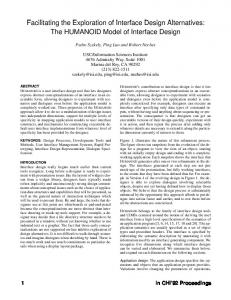
![UG086 Xilinx Memory Interface Generator (MIG), User Guide [PDF]](https://m.moam.info/img/260x300/ug086-xilinx-memory-interface-generator-mig-user-g_64798d2a098a9ee17d8b457c.jpg)