MIMAC: A Rate Adaptive MAC Protocol for MIMO ... - Cs.UCLA.Edu

MIMAC: A Rate Adaptive MAC Protocol for MIMO-based Wireless Networks UCLA Computer Science Department Technical Report # 040035 December 20, 2004

Gautam Kulkarni

Alok Nandan

Mario Gerla

Mani Srivastava

UCLA Electrical Engineering Dept.

UCLA Computer Science Dept.

UCLA Computer Science Dept.

UCLA Electrical Engineering Dept.

[email protected]

[email protected]

[email protected]

[email protected]

MIMAC: A Rate Adaptive MAC Protocol for MIMO-based Wireless Networks ABSTRACT This paper presents a rate adaptive medium access control (MAC) protocol for wireless networks with MIMO links. It is envisioned that the next generation high-throughput wireless LAN standard (IEEE 802.11n), which is currently under development, would use MIMO technology to achieve high data rates. An important design consideration is maintaining backward compatibility with the IEEE 802.11a/g standards. We adopt a joint MAC and physical layer strategy for channel access, based on the instantaneous channel conditions at the receiver. Our contributions include a transmit antenna and data rate selection scheme based on the optimal tradeoff between spatial multiplexing and diversity. The goal is to maximize the achievable data rate, given a MIMO channel instance and a target bit error rate. We also provide a feedback mechanism for the transmitter to obtain the rate selection settings from the receiver. Moreover, we maintain compatibility with legacy 802.11a/g devices and our protocol supports communication between devices with different number of antennas. The overall contribution is a MIMO physical layer aware, rate adaptive MAC protocol, which is compatible with 802.11a/g and can also be readily integrated with the 802.11n proposals.

Categories

&

Subject

Descriptors:

C.2.1

[Computer-Communication Networks]: Network Architecture and Design – wireless communication

General Terms: Algorithms, Performance, Design. Keywords: MIMO, MAC protocol, antenna selection.

1. INTRODUCTION The most prevalent wireless network technologies currently in use are based on the IEEE 802.11a/b/g [1, 2, and 3] standards and use CSMA/CA. The 802.11b technology offers a highest physical layer data rate of 11 Mbps, while 802.11a/g offer peak rates up to 54 Mbps. These are the rates at which bits are transmitted by the physical layer. The net throughput obtained, taking into account the overheads due to medium access control messages, channel contention and various preambles, is considerably less. Currently, efforts are on to develop and standardize the physical and MAC layer technologies for the next generation of wireless LANs. It has been stated in various proposals that the next standard, IEEE 802.11n, would support peak physical layer rates over 200 Mbps [4, 5]. The general consensus is the proposed use of Multi-Input

Multi-Output (MIMO) technology [6] at the physical layer to provide the high data rates that have been envisioned. There are still differences regarding the number of antennas to be used, the channel bandwidth and modulation / coding schemes. A practical issue in using multiple antennas is that for the antennas to be reasonably uncorrelated, they should be separated by about one wavelength. For the 5 GHz band, this corresponds to about 6 cm. Thus, small handheld devices could support at most 2 antennas while laptops could have 4 antennas. For the 2.4 GHz band, the wavelength is approximately double. In theory, if there are MT antennas at the transmitter and MR antennas at the receiver, the achieved data rate can be min (MT, MR) times that of the case with a single antenna at each end. These high data rates are obtained using the same spectrum and the same power levels. This gain is achieved by exploiting the multi-path diversity in a rich scattering environment. This paper presents joint MAC and physical layer design for MIMO-based wireless networks. The MAC is CSMA/CA based and an important design constraint is backward compatibility with 802.11a/g. We also show how our work fits in the context of the ongoing activity toward developing the 802.11n standard. Before we delve into the details of our design, we briefly review some prior work and explain the logical progression towards our approach. IEEE 802.11a/b/g support variable data rates, depending on the channel conditions. Auto Rate Fallback (ARF) [7] is a transmitter-oriented rate adjustment scheme. After a number of successful transmissions, the transmitter selects the next higher rate for subsequent packets. The transmission rate is reduced when the transmitter fails to receive two successful ACKs or if it fails to receive an ACK immediately after increasing the transmission rate. Receiver-Based AutoRate (RBAR) [8] is an improvement over ARF. RBAR is receiver-oriented and adjusts the data rate depending on the measured Signal to Interference and Noise Ratio (SINR) at the receiver. The rate is then communicated back to the transmitter. However, RBAR requires a modification to the control message formats. Opportunistic Media Access (OAR) [9] is a protocol that exploits the time-varying nature of the channel. The basic idea is to send multiple packets at high rate when the channel is favorable. The schemes described above were developed for Single Input Single Output (SISO) systems, or in other words, where both transmitter and receiver have a single antenna. The goal of our research is to present a rate-adaptive medium access protocol, which takes into account and exploits the underlying physical layer characteristics in a MIMO system. We also incorporate a feedback mechanism

into the MAC to convey certain channel characteristics from the receiver to the transmitter.

1.1 Paper Contributions The contributions of this paper are threefold: firstly, we present a physical layer scheme that maximizes the data rate for a target Bit Error Rate (BER) in a MIMO system. For a SISO system, this involves comparing the received SINR against various thresholds, corresponding to different modulation and coding schemes. In a MIMO system, there are several ways and modes of operation in which the multiple antennas can be used. We adopt the approach of transmit antenna and constellation selection. We select a subset of the total number of transmit antennas and choose the best constellation that can be supported on each of the selected antennas. Our results show that sending the maximum number of independent data streams (spatial multiplexing) is rarely the best strategy for maximizing the achievable data rate for a target BER and received SINR. Instead, the mode of operation that maximizes the data rate involves a tradeoff between spatial multiplexing and diversity. Secondly, we present the design of our MAC protocol, which maintains compatibility with 802.11a and provides the requisite feedback from the receiver to the transmitter to facilitate rate selection. Finally, our protocol is designed to function in a heterogeneous setting, i.e., nodes with different number of antennas are able to communicate with each other. The overall contribution is a MIMO physical layer aware, rate adaptive MAC protocol, which is compatible with 802.11a/g and can also be readily integrated with the 802.11n proposals.

1.2 MIMO Background We now give a very brief introduction to MIMO systems. For a given wireless communication link, both the transmitter and the receiver are equipped with multiple antennas. Depending on the mode of operation, independent or correlated data streams are sent by the transmitter on its antennas. At each of the receiver antennas, the received signal is a linear combination of the signals transmitted by the transmitter antennas. After performing some signal processing, the various transmitted streams are retrieved and decoded. The advantage of using MIMO is that either the quality of the link in terms of the BER or the data rate or a combination of both, are improved. The basic idea is to exploit multi-path propagation to our advantage by using the resulting diversity. There are different modes of operation of MIMO systems. •

•

Spatial multiplexing: In this mode, independent data streams are sent on the different transmitter antennas. Theoretically, with MT transmit antennas and MR receive antennas, a capacity gain of min (MT, MR) is obtained. Selection Diversity: In this mode, only one independent data stream is sent on the best antenna. This transmitreceive diversity gain is bounded by MTMR, the product

of the number of antennas at each end. Thus, for the same Signal to Noise Ratio (SNR), the BER is much less than that of a SISO system. Alternately, to maintain a target BER, the required SNR threshold is reduced. A direct consequence of this is increased transmission range without increasing the power. More recently, researchers have begun to examine more modes of operation that try to tradeoff capacity gain for diversity gain. The authors of [11] present an information theoretic study and obtain results that express capacity as a function of the diversity order.

[

Let x = x1 , x2,..., x M T

]

T

be the vector of transmitted symbols,

where each xi could, in general, be symbols from different constellations and y = [y1 , y 2 ,..., y M ] T be the vector of received symbols. Then we have: R

y = Hx + n

(1)

H is an MR×MT matrix whose elements are independent and identically distributed (i.i.d.) complex Gaussian random variables with zero mean and unit variance for Rayleigh fading channels. Each element H(i,j) is the fading parameter from transmit antenna j to receive antenna i. If the fading is correlated, then the elements H(i,j) are not independent random variables. The vector n is a complex Additive White Gaussian Noise (AWGN) vector. Thus, in a MIMO system the channel is represented by a matrix of random variables as opposed to a single random variable in a SISO system. This channel matrix is estimated by the receiver using training symbols sent by the transmitter. The transmitter has no knowledge of the H matrix, unless there is feedback from the receiver. Based on this, MIMO systems can be classified as Closed Loop (where transmitter has the channel state information – the H matrix) or Open Loop (where the transmitter has no knowledge of the H matrix). In closed loop MIMO systems, the transmitter can find the optimal power allocation for its antennas using a technique known as water filling [10]. However, the overheads due to the feedback of the H matrix are substantial as this involves quantization of MTMR complex random variables. The feedback operation has to be performed every time the channel changes in order to maintain fresh channel state information. For open loop MIMO systems, with equal power allocation on each transmit antenna, the well-known expression for the MIMO information theoretic capacity is: ρ ∗    H H   bits/s/Hz C = log 2 det  I M + M   

( 2)

where (*) denotes the transpose-conjugate, ρ is the SNR at any receive antenna and det(X) denotes the determinant of the matrix X. Equation (2) gives the information theoretic capacity, which is an upper bound on the achievable data rate. The data rates achieved in practical communication systems are considerably lower.

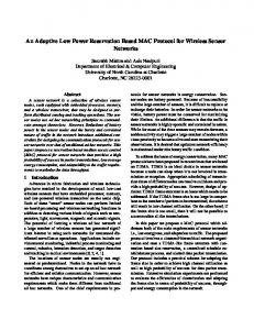
Feedback from RX Interleaver

Punctured convolutional encoder 1 Input

Separate

Map streams to antennas

into M streams

1

QAM Modulator 1

OFDM Modulator 1

QAM Modulator MT

OFDM Modulator MT

Feedback from RX Punctured convolutional encoder MT

Interleaver MT

Fig. 1a. Transmitter (TX) Structure Noise OFDM Demodulator 1

OFDM Demodulator MR

QAM Demodulator 1

Deinterleaver 1

Viterbi decoder 1

MIMO

Recombine to

MMSE

get transmitted

Receiver

QAM Demodulator M

Deinterleaver M

Viterbi decoder M

data

Feedback to TX

Antenna and constellation selection Fig. 1b. Receiver (RX) Structure

1.3 Related Work

conditions in a network.

We briefly summarize some prior related work. The works most closely related to ours at the physical layer are [11, 12, 13, and 14]. While the authors of [11], present information theoretic capacity results for the multiplexing-diversity tradeoff, the authors of [12, 13 and 14] study the tradeoffs for practical communication systems. The goal of [12, 13] is to select the best mode of operation, or in other words, selecting a subset of the transmit antennas and the appropriate QAM constellation [19], to minimize the BER for a given fixed data rate. In [12], depending on the channel state and the SNR, various conditions are derived to make a decision between spatial multiplexing and diversity. For example, in a 4 × 4 system, a data rate of 8 bits/sec/Hz can be achieved by sending either a 256-QAM constellation using the diversity mode or by sending 4 independent QPSK symbols on 4 transmit antennas. Each mode of operation will result in a different BER. The work in [13] is an extension of [12] to include operating points that tradeoff multiplexing and diversity. The authors of [13] and [14] were the first to demonstrate the multiplexingdiversity tradeoff for practical communication systems. The key contribution of [13] is showing that for a fixed rate, spatial multiplexing does not produce the best BER performance. We extend this concept to demonstrate that for a target BER and received SINR, spatial multiplexing is rarely the best way to maximize the data rate. Both [12] and [13] present strategies to minimize the BER for a given rate, while we try to maximize the achievable data rate for a target BER. This is a more useful problem to solve from the point of view of link adaptation under time varying channel

The work in [14] makes the following two contributions: firstly, for a given, fixed, data rate, the authors present an antenna and constellation selection method that maximizes the minimum SNR margin over all combinations of selected antennas and constellations that result in the given data rate. The SNR margin is the difference between the actual SNR and the required SNR threshold. In this aspect, [12], [13] and [14] are very similar. However, [14] takes into account the correlations between the antennas. Secondly, [14] also presents an antenna and constellation selection that maximizes the outage data rate for a given target SNR margin and an outage probability. An outage is said to occur when the SNR margin falls below the target SNR margin. The outage probability density functions are obtained empirically by simulating a large number of channels. Thus, in [14], antenna and constellation selection is done by using the statistical properties of various channel models. In contrast, we perform antenna and constellation selection based on the instantaneous channel state. In [15], the authors present a MAC protocol for ad hoc networks with MIMO links. A graph-coloring based approach is adopted with a very simple physical layer abstraction. As a result, they do not consider practical issues in a communication system such as constellation selection, support for variable rates, training symbols for channel estimation, etc. Moreover, their protocol is not compatible with the existing IEEE 802.11 MAC and they also require coordination between various links and perfect timing synchronization. The work in [16] is a generalization

of [15] for different classes of multiple antenna systems and follows a similar graph-coloring approach. In our work, we consider a realistic physical layer model and our MAC protocol is designed to be compatible with 802.11a/g and also supports nodes with different number of antennas. The two main 802.11n proposals provide various data rates corresponding to different combinations of constellations and number of independent data streams. The WWiSE proposal [4] only provides open-loop modes, i.e., there is no support for channel-state feedback from the receiver to the transmitter. The TGnSync proposal [5] provides optional beamforming modes, for which there is support for channel-state feedback. In our work we investigate the possibility of using transmit antenna selection for maximizing the data rate. This requires a new feedback mechanism, which can be incorporated in the TGnSync framework. Thus, our techniques are complementary to those proposed in [4] and [5] and can be easily integrated in [5] as an additional rate-adaptation scheme.

2. SYSTEM MODEL Consider a MIMO communication link with the transmitter having MT antennas and the receiver having MR antennas. Let ρ be the average input SNR at the receiver antennas. In a network setting with interfering links, ρ is the SINR. The receiver estimates the channel matrix, H, using the training symbols sent by the transmitter. We consider non-line-ofsight (NLOS) channels with Rayleigh fading with a low delay spread (≤ 50 ns). This corresponds to typical indoor office environments [17]. The basic transmission scheme is similar to that of IEEE 802.11a, which operates in the 5 GHz band. OFDM is used over channels of 20 MHz bandwidth and there are 48 data subcarriers and 4 pilot subcarriers. The guard interval is 0.8 µs. Since we consider low delay spread channels, the channel matrix is approximately constant over all subcarriers. For larger delay spreads corresponding to outdoor environments, rate adaptation needs to be done on a per-subcarrier basis. The same modulation and coding schemes as used in 802.11a are considered. The enhancement is that we now have multiple antennas and can send multiple data streams. We use a Minimum Mean Squared Error (MMSE) receiver [6] for MIMO decoding. Figure 1 shows a schematic diagram of the basic communication system. The input data is split into multiple streams. The number of streams and the constellation is determined from the feedback obtained from the receiver. The receiver computes this based on the measured SINR and using instantaneous channel knowledge. Each stream is then encoded using a punctured convolutional encoder [19] and QAM is used. We use the same modulation and coding schemes as 802.11a. A device with multiple antennas can communicate with an 802.11a device by using just one of its antennas. Another issue is that of devices with different number of

antennas. Small handheld devices could only support 2 antennas while larger devices such as laptops could have 4 antennas. These devices need to be able to communicate with each other and we design our protocol to be able to support that. In this paper, we consider two scenarios – a single link and a wireless LAN.

3. ANTENNA AND CONSTELLATION SELECTION We now answer the following question: •

For a given SINR, a target BER and knowledge of the instantaneous channel state, i.e., the H matrix, what is the highest data rate that can be achieved?

The best possible way to maximize the data rate is to send the entire channel state information back to the transmitter. The transmitter would then perform water filling and compute the optimal rate. We do not adopt this approach due to the high feedback overhead involved. Instead, we adopt the approach of antenna and constellation selection, using limited feedback, as was done in [12, 13 and 14] in different contexts, described in section 1.3. The idea is to select those antennas (a subset of the total number of transmit antennas) and constellations, which for the target BER, result in the highest aggregate data rate over all transmitted data streams. The question then is, why not send the maximum possible number of independent streams, i.e., min (MT, MR) streams (this is the spatial multiplexing mode)? The answer is that for a given SINR, target BER and a given instance of a channel matrix, spatial multiplexing rarely turns out to be the mode that maximizes the rate, as we shall show. The other extreme is sending just one independent stream. The diversity gain would then allow us to send higher order constellations. However, this is also not optimal in most cases. It turns out that in most cases, i.e., over most channel instances, some combination of multiplexing and diversity maximizes the data rate. An alternate approach might be to jointly encode the different data streams across multiple antennas. These codes are referred to as Space-Time Codes (STC) [6]. Space-time coding techniques can be used in addition to using 802.11a rates, as can be seen in the 802.11n proposals [4][5]. We, however, restrict ourselves to 802.11a constellations although our techniques are applicable for any QAM constellation. One more practical design issue that we consider is that the selected antennas must transmit equal power and use the same constellation. The reasons are as follows: a) reduction in the overhead of the feedback from the transmitter to the receiver, b) robustness to inaccuracies in channel estimates and c) reduction in the dynamic range requirements of power amplifiers. These issues were also identified in [14]. Structurally, our system shown in Figure 1 is similar to the systems in [13, 14]. The distinction is that our objective is

to maximize the data rate using instantaneous channel knowledge, the received SINR and a given target BER. The achieved data rate is the product of the number of streams selected times the data rate associated with the constellation that is selected. The received signal at any receiver antenna is a linear combination of the signals transmitted from the different transmit antennas. Firstly, they need to be “separated” into the individual streams. After that, the symbols are detected and decoded. Maximum Likelihood (ML) detection [19] is the optimal decoding method. However, the complexity is very high and hence we use a linear receiver followed by a symbol detector. In particular, we use the Minimum Mean Squared Error (MMSE) receiver. Let q be a Boolean vector of length MT. We set q(i) to be equal to one when transmit antenna i is selected and zero otherwise. When only M out of MT transmit antennas are selected, corresponding to the vector q, the effective channel matrix is denoted by H(M,q). When M (out of a possible min (MT, MR)) streams are sent, the post-processing SNR, i.e., the SNR at the input of the symbol detector (see Fig. 1(b)), for stream i is given by [6]: SNRi =

1 −1 −1  ρ   * H ( M , q) H ( M , q )    I M + M   i ,i 

(3)

where Ai,i denotes the (i,i) entry of the matrix A and ρ is the input SNR at the receiver antennas. Intuitively, we see that the SNR is “divided” over the M streams that are sent. Thus, sending the maximum number of streams for low values of ρ might not be the best strategy. Our results confirm this intuition. th

Now, since M has to be less than both MT and MR, we have the following number of combinations of transmit antennas that can be selected: MT   1

 MT  +    2

 M  + K +  T   K

  ≤ 2 M T − 1 

complexity O(n3), where n is the order of the matrix. The various IEEE 802.11n proposals also envision 2 × 2 or 4 × 4 systems, so the computational overhead of exhaustive search based rate selection is reasonable. Also, majority of the devices are most likely to be equipped with 2 antennas while access points would have 4 antennas. Moreover, as this would be a frequent operation, manufacturers can implement it in hardware. We now summarize our antenna and constellation selection algorithm. For M (number of antennas) from 1 to K = min (MT, MR) For each  M T M 

Calculate MMSE post-processing SNRs from (3) Compare minimum post-processing threshold to obtain constellation

This is a combinatorial problem and an exhaustive search yields the optimal solution. Since we consider devices with a maximum of 4 antennas, the maximum number of combinations we need to examine is 15, which corresponds to the 4 × 4 case. Each combination requires matrix multiplication followed by inversion, which results in a

SNR

to

Total rate = Selected constellation × M Select highest total rate and store corresponding M and q If multiple solutions are found, use the M and q that has the highest SNR margin (difference between the minimum postprocessing SNR and the threshold). This algorithm is used at the receiver and the results, M and q, are fed back to the transmitter. Table I shows the set of physical layer data rates that can be achieved. Thus, with sufficient SNR, it is possible to obtain peak physical layer rates of up to 216 Mbps using the same modulation and coding schemes of 802.11a and using 20 MHz bandwidth. More QAM constellations using 5/6 and 7/8 coding rate as well as 40 MHz channels can also be used as in [4, 5] but we choose to use only the 802.11a/g rates in order to illustrate the gain achieved using MIMO. Our techniques are equally applicable for other QAM constellations and the use of 5/6 and 7/8 coding rate will result in further performance enhancement. Table I. Achievable set of data rates

( 4)

where K = min (MT, MR). For each combination of selected antennas, the lowest post-processing SNR is compared against various thresholds corresponding to different data rates for a target BER. The data rate achieved is the product of the number of antennas times the rate that can be supported by the lowest post-processing SNR. This is due to the restriction of using the same constellation on each of the selected antennas. The important point here is that postprocessing SNR is compared with the thresholds, and not the SNR measured at the receiver antennas.

 combination with M selected antennas  

802.11a rates (Mbps) 6

Coding

MIMO rates with

Modulation

Rate

1, 2, 3, 4 streams (Mbps)

BPSK

1/2

6, 12, 18, 24

9

BPSK

3/4

9, 18, 27, 36

12

4-QAM

1/2

12, 24, 36, 48

18

4-QAM

3/4

18, 36, 54, 72

24

16-QAM

1/2

24, 48, 72, 96

36

16-QAM

3/4

36, 72, 108, 144

48

64-QAM

2/3

48, 96, 144, 192

54

64-QAM

3/4

54, 108, 162, 216

In a time-varying channel, antenna and constellation selection must be performed as the channel changes. The results need to be fed back to the transmitter. The next section describes the necessary MAC modifications.

4. MAC PROTOCOL DESIGN In this section we describe our MAC protocol – MIMAC (short for MIMO MAC). MIMAC uses physical layer information to optimize MAC layer throughput.

8 us

L−STF

8 us

4 us

L−LTF

L−SIG

8 us

HT−SIG

2.4 us

7.2 us

7.2 us

HT−STF

HT−LTF

......

HT−LTF

N = Number of Antenna

BPSK r = 1/2

4.1 MIMAC Protocol MIMAC is a receiver oriented rate adaptive MAC protocol. In a SISO system, the SINR is a sufficient metric for evaluating channel quality and hence determining the rate that can be supported. In a MIMO system, both the SINR and the channel matrix have to be known at the receiver. The channel matrix is estimated using the training symbols sent by the transmitter. Once the SINR and channel are known at the receiver, antenna and constellation selection can be performed. The key features of the MIMAC protocol are as follows: •

The receiver-based channel quality estimation and antenna and constellation selection mechanism.

•

An efficient feedback mechanism to convey the antenna selection to the transmitter.

•

The MIMAC protocol can be implemented in the current IEEE 802.11 with minimal changes, providing seamless interoperability with 802.11 legacy devices.

•

Control messages (RTS / CTS / ACK) are always sent using a single antenna

•

Can be integrated with the 802.11n proposals

We assume the DCF mode of operation of the 802.11 standard. In MIMAC, the packets carry feedback from the receiver in the form of the constellation selected and the antenna mask, which specifies the exact antenna configuration to be used for the particular transmission. This information is termed as limited feedback, since we are not sending the complete channel state information to the transmitter. The advantages of this type of feedback are having a low overhead, and at the same time providing enough information to the transmitter to perform rate adaptation exploiting current channel information. The low overhead assumes further importance since this information is to be sent periodically and at the base rate for interoperability reasons. The transmitter (SRC) initially sends the RTS at the base rate on a single antenna. There are two possibilities for the choice of the “base” rate - 6 Mbps or 54 Mbps and both are examined in the two proposals. Using 6 Mbps allows transmission over a longer range but also adds to the control overhead. On the other hand, use of 54 Mbps may not be possible for long ranges. Based on the channel conditions we use 6 Mbps or 54 Mbps. The rate is carried in the physical layer preamble, which is always sent at the lowest rate. The receiver (DST) receives the RTS and responds with a CTS packet. For the very first packet, the receiver has no knowledge of the channel matrix because it has not received training symbols from the transmitter.

RATE

LENGTH

ANTENNA MASK

BITS :

4

18

4

Tx

RESERVED

CRC

TAIL

8

6

ANTENNA

2

6

Figure 2: PLCP Header Packet Format

Thus, SRC sends the first DATA packet using the maximum possible number of streams and the highest rate. This is analogous to ARF in which the transmitter initially starts with the highest rate. Upon receiving the training symbols and using the measured SINR, DST determines the rate and sends the antenna and constellation information back to SRC in the PLCP header of the ACK frame, as we shall describe in section 4.3. Each node maintains a data structure called Preferred Rate Cache (PRC), that indicates the preferred data rate and antenna configuration that should be used for the purpose of communicating with the destination node. Each entry in the PRC contains the data rate, the antenna mask and the constellation that was computed based on the training symbols and antenna information received in earlier successful transmission from that node. Modifications to the existing 802.11 frames for MIMAC are minimal.

4.2 Incorporation into IEEE 802.11 PHY One of the key design goals of the protocol is to maintain interoperability with legacy 802.11 devices. To that end, we adopt an enhanced preamble design that achieves this goal and at the same time, provides a mechanism to convey the feedback information with minimal overhead. We choose to send the feedback in the PLCP header of the ACK frame since the physical layer uses this information. The enhanced preamble design proposed in MIMAC is similar to TGnSync‎ proposal [5], except for the feedback mechanism and a new mechanism for reducing the physical layer overhead, which we describe below. Figure 2 shows the PLCP header format for the various frames. The length of the preamble increases with the number of antennas used by the node participating in the transmission. We use similar notation as [5] to refer to the various fields in the PLCP header. The legacy preamble fields transmitted are denoted by L-STF (Legacy-Short Training Fields) L-LTF (Legacy-Long Training Fields) and L-SIG (the legacy SIGNAL field). The purpose of having the legacy SIGNAL field and training symbols is to facilitate communication when legacy 802.11a devices are present in the neighborhood. When two MIMO devices

communicate, the rate and length fields in the legacy PLCP header may not always give the same duration as the HT (High Throughput) SIGNAL field. This causes the legacy devices to be in the receive mode and remain silent during the MIMO communication dialogue. This is referred to as “spoofing” in [5]. We need to send extra training symbols for the higher throughput or MIMO case, which are referred to as HTSTF and HT-LTF for High Throughput Short and Long Training Fields respectively. The number of HT-LTF fields depends on the number of antennas, or in other words, the number of spatial streams used for transmission. In our protocol we send the RTS/CTS/ACK frames using a single antenna, so the HT-LTF field will be just one in number. However, the DATA frame will contain variable number of HT-LTF fields depending on the number of streams used in the transmission, which in turn is computed by our antenna selection algorithm. Note that when a MIMO device communicates with a legacy 802.11a device, it does not send the HT SIGNAL and preambles. The HT-SIG field of the PLCP header is used to exchange the antenna information. The Rate and Length fields are used for the normal operation as in the 802.11 protocol. We add two new fields; viz., Antenna Mask (ANT-MASK) and number of transmit Antenna (TX-ANT). The Antenna mask is 4 bits in length because 4 antennas is the maximum envisioned by the two major 802.11n proposals. This is due to the form factor of laptops and the minimum separation requirement for adjacent antennas placement. Consequently the TX-ANT field is 2 (i.e., log (4)) bits in length. We have a RESERVED field of 6 bits for future use. The ANT-MASK field is set to the antennas selected and the TX-ANT is set to the number of antennas that the device supports, in the DATA frame sent. The receiver measures the SINR and uses the training symbols to determine the optimal antenna and constellation using the algorithm described in section 3. The receiver then conveys the optimal antenna selected in the ANT-MASK field of the PLCP header of the ACK frame. All subsequent transmissions are done using the antennas selected. It is a physical layer requirement to send one HT-LTF for every stream sent over a separate antenna. Each HT-LTF has duration of 7.2µs, which presents a significant overhead in itself. A 1460 byte packet at 216 Mbps takes approximately 54µs to transmit. Thus, at very high physical layer data rates, the overheads due to preambles and control frames are much higher. A consequence of using a subset of transmitter antennas is reduction in the HT-LTF overhead. This is an added advantage of using antenna selection. However, as the channel changes with time, the channel matrix must be reestimated periodically. This requires sending training symbols on all transmit antennas. An interesting question that now arises is how frequently should the HT-LTF be sent over all antennas, since they present a significant

overhead? That depends on the coherence time of the channel. For the 5 GHz band and for low mobility scenarios and data rates of 54-216 Mbps range and for a typical packet size of 1000 bytes, the coherence time is of the order of several tens of packet transmission times. As a rule of thumb, we performed the re-estimation every 10 transmissions of the DATA frame. Another option, which we have left open in the design, is the RESERVED bits in the PLCP Header. For example, in the HT-SIG field one bit in the RESERVED field can be used as a flag to convey to the sender that it needs to send the LTF’s due to sudden channel state variation as observed by the receiver.

5. EFFICIENCY ANALYSIS In this section, we compute the efficiency of our MAC protocol. We begin with the computation of the expected data rate of a single transmitter-receiver pair by taking into account the channel properties. A transmission dialogue is defined to be the sequence RTSCTS-DATA-ACK or DATA-ACK, depending on whether or not the RTS is enabled. Every MAC frame is preceded by a physical layer preamble and the PLCP header. The MAC headers are the same as that in 802.11a, but the preambles and the PLCP header have been modified. The overhead due to the training symbols, in particular the HTLTF, depends on the number of antennas selected. When RTS / CTS are used, the normalized goodput (S) is given by S=

E [H ] (5) TIdle + TRTS / CTS + TSIFS + TACK + 2τ + TPLCP (n ) + 3TPLCP (1) + E [H ]

T RTS / CTS = TRTS + τ + TSIFS + TCTS + τ + TSIFS TPLCP (n) = TLegacy + THT − SIG + THT − STF + n × THT − LTF

(6) (7 )

T Idle = TDIFS + TCW where E[H] is the expected payload duration,

(8)

τ is the propagation delay, TPLCP(n) is the duration of the physical layer preamble and the PLCP header when n transmit antennas are selected, TRTS/CTS denotes the MAC overhead due to RTS and CTS, TRTS, TCTS and TACK are the durations of the MAC portions of RTS, CTS and ACK, respectively, TSIFS and TDIFS are the durations of the SIFS and DIFS, respectively, and TCW is the average time spent in the backoff process. For the 2 node case, there is no contention with other transmitters and

TCW ≈ 0.5 × CW min × slot duration

(9)

TLegacy includes the duration of the legacy preamble and the legacy SIGNAL field. All SIGNAL fields are sent at 6 Mbps (BPSK, rate = 1 / 2) and the control messages are sent at 54 Mbps (64-QAM, rate = 3 / 4) using a single antenna. The RTS MAC header consists of 20 octets, CTS and ACK are 14 octets each and

the MAC header of DATA consists of 28 octets. As in 802.11a, we have TSIFS = 16 µs, slot time = 9 µs, CWmin = 15 and DIFS duration = 34 µs. TLegacy and THT-SIG add up to 28 µs while THT-STF is 2.4 µs and THT-LTF is 7.2 µs [5]. The value of E[H] depends on the data rate, which in turn depends on the SNR and the channel conditions, i.e., the H matrix. In a SISO system, the value of the measured SNR is sufficient in selecting the data rate, by comparing it to the corresponding threshold. First, let us recall some results that apply to SISO systems. Let p(r) be the probability that rate r is chosen. Rate r is chosen when the received SNR lies in a certain range. For example, p (r = 0) = prob(SNR < SNR6 )

p (r = 6) = prob(SNR6 ≤ SNR < SNR9 )

(10)

M p (r = 54) = prob( SNR54 ≤ SNR)

Where SNRr denotes the SNR threshold corresponding to data rate r. The average transmission rate is given by SISO ravg = ∑ ri p(ri )

(11)

i

In MIMO systems, the situation is a little more complicated, as was discussed in section 3. We now approximate the MIMO data rate to be equal to min(MT, MR) times the SISO data rate for a given SINR. This is because intuitively, MIMO increases the channel capacity by the factor min(MT, MR) for the same SINR. Thus, to obtain the average MIMO transmission rate, we first calculate the average SISO rate and multiply it by the factor min(MT, MR). In Rayleigh fading channels, the received signal amplitude has a Rayleigh distribution, whereas the received signal power and hence the receiver SNR has an exponential distribution. If the transmitted power is P, the transmitter-receiver distance d, path loss exponent β, and noise power No, the received SNR is Pd − β α SNR = No

(12)

transmission of a sequence of physical data frames to the same receiver back-to-back) improves the goodput. Table II. Average physical layer data rates Distance (meters)