Minimal Models and Canonical Neural Computations

Forthcoming in Synthese

M. Chirimuuta

Minimal Models and Canonical Neural Computations: The Distinctness of Computational Explanation in Neuroscience

Penultimate version M. Chirimuuta ([email protected]) History & Philosophy of Science, University of Pittsburgh

Abstract In a recent paper, Kaplan (2011) takes up the task of extending Craver’s (2007) mechanistic account of explanation in neuroscience to the new territory of computational neuroscience. He presents the model to mechanism mapping (3M) criterion as a condition for a model’s explanatory adequacy. This mechanistic approach is intended to replace earlier accounts which posited a level of computational analysis conceived as distinct and autonomous from underlying mechanistic details. In this paper I discuss work in computational neuroscience that creates difficulties for the mechanist project. Carandini and Heeger (2012) propose that many neural response properties can be understood in terms of canonical neural computations. These are “standard computational modules that apply the same fundamental operations in a variety of contexts.” Importantly, these computations can have numerous biophysical realisations, and so straightforward examination of the mechanisms underlying these computations carries little explanatory weight. Through a comparison between this modelling approach and minimal models in other branches of science, I argue that computational neuroscience frequently employs a distinct explanatory style, namely, efficient coding explanation. Such explanations cannot be assimilated into the mechanistic framework but do bear interesting similarities with evolutionary and optimality explanations elsewhere in biology.

1


M. Chirimuuta

I. Introduction If any perspective in philosophy of neuroscience can today claim to be dominant, it is the mechanistic one. The new mechanists have successfully displaced their reductionist and eliminativist predecessors, and have demonstrated the virtues of the mechanistic approach when discussing numerous examples across the board from molecular to behavioural neuroscience 1 . Yet before the mechanist orthodoxy becomes so entrenched as to be untouchable, it is worth considering its limitations (cf. Chemero and Silberstein 2008, Weiskopf 2011a). A particular point of controversy is over whether the new mechanists successfully describe explanatory practice in all subfields of neuroscience, from the molecular to the behavioural, and whether mechanistic norms of model building which emphasise decomposition into small working parts are appropriate for the “higher level” branches of systems and cognitive neuroscience, and to the methodologically diverse branches of computational neuroscience. The term “computational neuroscience” labels a broad research area which uses applied mathematics and computer science to analyze and simulate neural systems. The techniques and explanatory practices of this field are discussed in detail by Kaplan (2011) 2 . In particular, Kaplan argues that models in computational neuroscience should be subject to the same mechanistic explanatory norms that have been formulated for other branches of neuroscience (Craver 2006, 2007). In other words, computational neuroscience should not be treated as a distinct field with its own explanatory norms: computational explanation in neuroscience is a 1

Just a small sampling of works: Bechtel and Richardson (1993), Machamer et al. (2000), Craver and

Darden (2001), Craver (2006, 2007), Bechtel (2008), Bogen (2008), Bogen and Machamer (2010), Kaplan and Craver (2011) and Piccinini and Craver (2011). 2

In what follows I focus on this particular presentation of the mechanistic approach to computational

neuroscience and cognitive science. For work in a similar vein see Piccinini (2007), Piccinini and Craver (2011), Kaplan and Craver (2011), Piccinini and Bahar (2013). The view I develop here is directed at this general view, to the extent that it presupposes the two mechanistic norms that I outline below (3M and MDB), but for ease of exposition I only make explicit the contrast with Kaplan’s (2011) paper. Note that not all mechanists are committed to the narrow view of mechanistic explanation that is targeted here. See e.g. Bogen and Machamer (2010).

2


M. Chirimuuta

species of mechanistic explanation (p. 339). In this paper I will be arguing for an alternative approach. Contrary to Kaplan, Piccinini and Craver, I propose that computational explanation in neuroscience be treated differently from mechanistic explanation. Following Dayan and Abbott (2001:xiii), I hold that computational models are often interpretative, as opposed to phenomenal or mechanistic. Interpretative models are central to explanations of why a particular neuronal type or brain area is organised in a certain way, explanations which typically make reference to efficient coding principles. In contrast, phenomenal models describe what is there, and mechanistic models explain how systems work. Informationtheoretic and computational principles are central to interpretative modelling, and causal-mechanical descriptive detail and accuracy is not required. For this reason, most interpretative models are minimaI. That is to say, they typically abstract away from many biophysical details of the neural system, in order to highlight dominant causal influences or universal behaviour I present a new class of minimal model – the I-minimal model – which figures heavily in the efficient coding explanations that are prevalent in computational neuroscience. In order to illustrate this distinct explanatory pattern I will present a pair of case studies. Firstly, I discuss the influential contrast normalisation model of primary visual cortex (Heeger 1992), which has recently been interpreted as a canonical neural computation (Carandini and Heeger 2012) – one of a few basic computational operations that are frequently found in different neural circuits, and are described at a high level of abstraction from biophysical implementation. The second example is the much-used Gabor model of V1 receptive fields. Models similar to this one have been described by Kaplan (2011) as merely phenomenal and not explanatory. I will show how the Gabor model is able to answer important explanatory questions, including Woodward’s (2003) “what-if-things-had-been-different questions”, even though it departs fully from the model-to-mechanism mapping framework that has been proposed as the criterion for explanatory success (Kaplan 2011, Craver and Kaplan 2011). In the next two sections I will present Kaplan’s case against the distinctness of computational explanation (section 2) and in favour of the universality of mechanistic explanation (section 3). Section 4 will introduce canonical neural computations and

3


M. Chirimuuta

the normalisation model. Section 5 will analyse the explanatory form employed in this kind of computational modelling, presenting the example of the Gabor model. In the final section I consider the lessons to be learned, in particular the new picture of levels that emerges – levels as perspectives rather than levels of scale or levels of being, as typically conceived. This gives us new insight into the utility of computational modelling as a distinct practice within neuroscience.

2. Claims of “Computational Chauvinism” Before presenting his positive thesis, Kaplan first removes one potential obstacle to the mechanistic account of computational neuroscience, namely an influential view in the philosophy of mind and philosophy of psychology which sees computational explanation as exclusive to psychology and autonomous from neuroscience. Following Piccinini (2006), Kaplan (2011:341) employs the term “computational chauvinism” to cover this view which takes computational models and explanations to be independent from mechanistic ones, and therefore subject to different norms. He discusses three “interrelated claims” which constitute the chauvinist3 position attributed to Johnson-Laird (1983) and Fodor (1975): C1 (Autonomy) – “Computational explanation in psychology is autonomous from neuroscience.” C2 – “[C]omputational notions are uniquely appropriate or proprietary to psychology” C3 (Distinctness) – “[C]omputational explanations of cognitive capacities in psychology embody a distinct form of explanation – functional analysis or functional explanation.”

3

It is not clear whether or not, each of these theses is sufficient for computational chauvinism, or if

they are jointly sufficient, or if any of them are necessary. In proposing my own view on the explanatory models in computational neuroscience, I will endorse modified versions of C1 and C3.

4


M. Chirimuuta

What is striking is that the idea that computational explanation in neuroscience may be distinct from mechanistic explanation is only presented as part of a package of contentious views about the independence of psychology from neuroscience, such as the idea that computational notions are tied exclusively to psychology (C2). As Kaplan notes (p.342), C1-3 imply that there can be no such thing as explanatory computational neuroscience! Furthermore, the very existence of computational neuroscience refutes C2, a thesis proposed by Fodor (1975). Thus it is not hard to find reasons to reject the thesis of non-mechanistic computational explanation, as it is presented here. Firstly, the autonomy claim of C1 is given a very strong sense of psychology going about its business in utter isolation from neuroscience. Most would agree that in the last three decades cross talk between these disciplines has been continually increasing, and that it has been scientifically fruitful. In particular, the birth of cognitive neuroscience as a field in its own right (see Gazzaniga et al. 1998), and the explosion of methods in human neuroimaging has further blurred disciplinary boundaries. C1 is also associated with the functionalist’s strong thesis of the multiple realizability of the mental in completely non-biological systems. This thesis entails that one could develop a flourishing computational science of the mind/brain in isolation from neuroscience, and it has been rightly challenged (e.g. Bechtel and Mundale 1999). But it should be noted that there is a weaker claim in the vicinity of C1 which Kaplan does not discuss. Namely, the thesis that there are computational explanations in psychology or neuroscience that are not tied to any particular neural realization. Such explanations refer to a prominent functional feature which may be instantiated by a number of different biophysical mechanisms, and so is multiply realized in a weaker sense (Weiskopf 2011b). The picture that follows is one of computational descriptions that are fairly independent but still loosely constrained by the capacities and limitations of biophysical processes. In Section 5 I will make the case that this is how we should interpret canonical neural computations, such as normalization. C2 would find few apologists these days, for the reason that computational modelling is now ubiquitous in neuroscience as well as psychology and cognitive science. C3, the thesis of a distinct computational explanatory strategy, is more

5


M. Chirimuuta

promising. Like Piccinini and Craver (2011), Kaplan ties the distinctness thesis to Cummins’ (1983) notion of functional analysis. Kaplan argues that since Cummins’ functional explanations must eventually refer to mechanisms, they are not truly distinct from mechanistic explanations (p.345). Whatever the pro’s and con’s of Cummins’ account, C3 like C1 can be repackaged as a perfectly sensible thesis regarding explanation in computational neuroscience. In Section 5 I will argue that many computational models are developed in order to address specific questions about the role of particular neurons or circuits in coding and information processing required for particular tasks. As Dayan and Abbott (2001:xiii) describe, this class of “interpretative” models is important in asking “why” questions regarding the function and coding properties of neural structures. Addressing the “what” (descriptive models) and “how” (mechanistic models) can only get you so far4. Brandon (1981:91) made an analogous point regarding teleological explanation in biology: In adult Homo sapiens there are marked morphological differences between the sexes. Why is this? Answer: Different sex specific hormones work during ontogenetic development to produce these differences. Is this answer satisfying? That depends on the question one’s really asking. One might be asking what’s behind these hormonal differences, what’s it all for. Whether of not this question is interesting or answerable, it is not answered by the above bit on hormones. One might want more. Similarly, imagine if neuroscientists had only descriptive and mechanistic models of the action potential. They would know what an action potential is, and how it is generated, but that does not entail that they know anything of its function – what it’s for. Without this crucial piece of theory there would be no way to connect 4

Rather tellingly, Kaplan (2011:349) quotes from Dayan and Abbott (2001: xiii) in order to invoke

their distinction between descriptive and mechanistic models; but this third class of models gets no mention whatsoever. In comparison, Craver (2007:162) acknowledges that there may also be nonmechanistic (“non-constitutive”) explanation in neuroscience, but restricts his focus. I.e. he accepts the possibility of explanatory pluralism. It might be argued, in a similar vein, that the I-minimal models I discuss below are not counter-examples to Kaplan’s account because they are simply beyond his focus. But that would be to ignore his explanatory monism (the claim that all explanatory models in computational neuroscience are mechanistic).

6


M. Chirimuuta

neuroanatomy and neurophysiology to function and hence to behaviour – seeing, smelling, remembering. A central dogma of neuroscience is that the action potential is for information transmission, and that information theory and computational principles are needed to understand why action potentials have particular patterns of generation5. Below, I will show that while computational explanation in neuroscience is not entirely insulated from mechanistic considerations, it does have a distinct explanatory form. Thus it should not be subject to mechanistic norms of explanation. Next I will discuss Kaplan’s presentation of those norms.

3. Minimal Models or More Details the Better? The essence of Kaplan’s conception of mechanistic norms is captured by the modelto-mechanism-mapping (3M) requirement: (3M) A model of a target phenomenon explains that phenomenon to the extent that (a) the variables in the model correspond to identifiable components, activities, and organizational features of the target mechanism that produces, maintains, or underlies the phenomenon, and (b) the (perhaps mathematical) dependencies posited among these (perhaps mathematical) variables in the model correspond to causal relations among the components of the target mechanism. (Kaplan 2011:347, cf. Kaplan and Craver 2011:6116) 5

Piccinini and Scarantino (2010) are careful to distinguish computation from information processing.

This distinction is not critical for understanding the scientific material discussed below because these neuroscientists are not associating “neural computation” with digital computation, or any other manmade computational system. Rather “neural computation” is a catch-all for whatever information processing (i.e. formally-describable input-output transformations) neural systems do and the theoretical definition of neural computation is a work in progress. 6

Crucially, Kaplan and Craver’s (2011:611) version of 3M lacks the qualificatory phrase “to the extent

that”. They write that: “In successful explanatory models in cognitive and systems neuroscience (a) the variables in the model correspond to components….”. This can reasonably be interpreted as requiring that all components correspond to mechanism parts, thus requiring that models contain no non-referring mathematical features such as dummy variables or un-interpretable parameters. This is a problematic requirement that Kaplan (2011:347-8) avoids, stating just that at least one model variable or dependency must correspond to a mechanism component or causal relations.

7


M. Chirimuuta

It is important to make a few clarificatory points about 3M. Firstly, Kaplan (2011:347, following Weisberg 2007) describes it as a “regulative ideal”, i.e., “as a clear guideline for the construction of explanatory mechanistic models in computational neuroscience and a standard by which to evaluate them as explanations”. This suggests that for any model whose variables represent a few mechanism components, any more detailed model, accurately describing more components, will – all else being equal – be better. Thus the hypothetical, maximally complete and detailed representation of the mechanism is the one best explanatory model onto which all others aim to converge. Kaplan (2011:347) is careful to note that: “3M does not entail that only completely detailed, non-idealized models will be explanatorily adequate. 3M is perfectly compatible with elliptical or incomplete mechanistic explanations, in which some of these mechanistic details are omitted either for reasons of computational tractability or simply because these details remain unknown.” What 3M does imply, however, is that adding detail to a model will typically make it a better explanation. As Kaplan (2011:347) writes, “3M aligns with the highly plausible assumption that the more accurate and detailed the model is for a target system or phenomenon the better it explains that phenomenon, all other things being equal.”7 I call this the More Details the Better (MDB) assumption8. So while 7

Unfortunately Kaplan gives no indication of how the “all else equal” clause should be spelled out.

Given that he only mentions idealization and abstraction as there for “computational tractability” or because the details are unknown, I assume that the “all else equal” clause” just means that if the choice is between a fully detailed model which is impossible (or very difficult) to implement in your hardware, or an elliptical model that works, the elliptical model is better. 8

As I see it, the primary statement of the MDB assumption is in Craver’s (2007:113) discussion of the

“mechanism sketch”, as part of his presentation of the norms for mechanistic explanation: “A mechanism sketch is an incomplete model of a mechanism. It characterizes some parts, activities, or features of the mechanism’s organization, but it leaves gaps. Sometimes gaps are marked in visual diagrams by black boxes or question marks. More problematically, sometimes they are masked by filler terms that give the illusion that the explanation is complete when it is not. …. Terms such as ‘‘activate,’’ ‘‘inhibit,’’ ‘‘encode,’’ ‘‘cause,’’ ‘‘produce,’’ ‘‘process,’’ and ‘‘represent’’ are often used to indicate a kind of activity in a mechanism without providing any detail about exactly what activity fills that role. Black boxes, question marks, and acknowledged filler terms are innocuous when they stand

8


M. Chirimuuta

mechanists nod to the importance of abstraction and idealization9, they see them as no more than pragmatic constraints necessitated by gaps in the data, hardware restrictions (how much detail current computers can simulate), or our cognitive limitations (how much detail in a model we can make sense of). Kaplan (2011:347) rightly notes that Batterman (2009) expresses an opposing view whereby abstraction and idealization can actually contribute to the explanatory success of a model. Batterman’s (2002) account of the explanation of critical phenomena in thermodynamics highlights minimal models -- those which exclude microphysical detail irrelevant to the understanding of physical behaviours such as phase transitions. In other words, this is the view that there are in-principle reasons why scientists will build incomplete models. Crucially, though, this is not simply the opinion of an iconoclastic philosopher of physics; it is actually a view that one finds articulated frequently in the computational neuroscience literature. So in the remainder of this section I will contrast the More Details the Better, “maximalist” account with the minimalist alternative. This contrast is an important preliminary to the case studies and new account of explanatory norms which will be developed in subsequent sections. In sum, 3M and MDB are the twin pillars of Kaplan’s mechanistic approach to computational neuroscience. It is worth mentioning the proposed advantages of this account. Firstly, it is said to allow for a robust distinction between merely phenomenal and truly explanatory models unlike, e.g., Chemero and Silberstein’s (2008) dynamic systems approach; similarly, it fits with the common mechanist intuition that how-actually models provide better explanations than how-possibly as place-holders for future work….”. In general terms, better explanations arise as research progresses along the axis from mechanism sketches, to mechanism schemata, and finally to complete mechanistic models. On most occasions in which the MDB assumption is in play, a mechanism sketch is held up to unfavourable comparison against an improved, more detailed model. See discussion below of the Hodgkin-Huxley model, and Kaplan’s (2011) other case studies of progress in model building through de-idealization. 9

A note on terminology: by ‘abstract’ I mean a model which leaves out much biophysical detail, in

other words ‘highly incomplete’; by ‘idealized’ I mean a model which describes a system in an inaccurate or unrealistic way (Thomson-Jones 2005). In criticizing the MDB assumption, abstraction is the more relevant term. However, the literature on models often conflates these two.

9


M. Chirimuuta

models. Also, it is said to fit with the de-idealising trajectory of a number of research projects in computational neuroscience. Kaplan presents three case studies – action potential models beginning with Hodgkin and Huxley (1952), the Difference of Gaussians model of retinal ganglion cell receptive fields, and the Zipser-Anderson gain field model of motor control – which are intended to show that neuroscientists are in the business of incrementally improving the explanatory success of their models by adding more accurate biophysical detail as soon as new neuroscientific facts are discovered. Some high-profile research programmes in neuroscience do conform to the MDB methodological prescription. For example, the Human Brain Project is a new Europe-wide flagship project which has the stated goal of simulating an entire human brain in a super-computer (see http://www.humanbrainproject.eu/). This is a followon from the Blue Brain Project, which aims to produce highly realistic and detailed computer simulations of individual cortical columns (Markram 2006; see http://bluebrain.epfl.ch/). Such projects are obviously animated by the idea that building computational models which simulate actual neural mechanisms with as much detail and accuracy as currently possible will be an invaluable means to link neural circuits to behaviour and to understand the functioning of the healthy and diseased brain. On the other hand, it is by no means difficult to find computational neuroscientists criticising the MDB methodology. Commonly, pragmatic concerns are discussed in the same breath as in principle ones. It is perhaps for this reason that such concerns have been ignored by mechanist philosophers of neuroscience writing in favour of MDB – for if the only reasons not to build a maximally detailed model are merely pragmatic, these are deemed irrelevant to the normative project of philosophy of science. In a recent textbook, Sterratt et al. (2011:316) articulate the practical worries over maximalist modelling: “[T]o make progress in the computational modelling of biological systems, abstraction of the elements of the system will be required. Without abstraction, the resulting models will be too complex to understand and it will not be feasible to carry out the desired computations even using the fastest computers…” (cf. Sejnowski et al., 1988:1300)

10


M. Chirimuuta

Similarly, in the textbook Fundamentals of Computational Neuroscience, Trappenberg (2010:7) writes that, “[m]odelling the brain is not a contest in recreating the brain in all its details on a computer. It is questionable how much more we would comprehend the functionality of the brain with such complex and detailed models.” But in the same passage Trappenberg suggests that complex systems can, in principle, be better explained by modeling only the essential details: “Models are intended to simplify experimental data, and thereby to identify which details of the biology are essential to explain particular aspects of a system.” (p.6) And in a seminal paper outlining methodological and explanatory aims and achievements of the then new field of computational neuroscience, Sejnowski, Koch and Churchland (1988:1300) make the connection between minimal modelling in physics, and the value of abstraction (and to some extent, idealization) in neuroscience: “Textbook examples in physics that admit exact solutions are typically unrealistic, but they are valuable because they illustrate physical principles. Minimal models that reproduce the essential properties of physical systems, such as phase transitions, are even more valuable. The study of simplifying models of the brain can provide a conceptual framework for isolating the basic computational problems and understanding the computational constraints that govern the design of the nervous system.” At this stage it is important to note that there are two different notions of minimal models currently in play in the philosophy of science literature. In Batterman’s account, the explanations which utilize minimal models are not causal-mechanical ones. In contrast, Weisberg (2007) uses the term ‘minimal model’ to refer to models which accurately capture essential causal detail – the “difference makers” (Strevens 2004, 2008) – and hence still provide a kind of causal-mechanical explanation. The contrast is significant enough to warrant the introduction of disambiguating labels: Bminimal models

for

the

Batterman

type,

and

A-minimal models

for

the

Strevens/Weisberg type. We have seen that computational neuroscientists talk approvingly of minimal models; the further question of whether these models figure

11


M. Chirimuuta

in causal-mechanical or some other kind of explanation will be important to our subsequent discussion of the adequacy of the mechanistic framework in these cases. For instance, Levy (forthcoming) uses a study of the Hodgkin-Huxley model of the action potential to argue convincingly against the MDB assumption. Levy and Bechtel (forthcoming; cf. Levy forthcoming) show how numerous mechanistic explanations in neuroscience and biology utilize A-minimal models, and that the explanatory value of these models would not be enhanced by the addition of further biophysical detail. Thus one can reject MDB but still accept the broader mechanistic explanatory framework. In sum, the existence of A-minimal models in computational neuroscience does not rule out Kaplan’s central claim that computational explanation is a species of mechanistic explanation. So the task of the next two sections will be to present examples of influential models in computational neuroscience which, as I will argue in section 5, are minimal but not mechanical. Thus I will describe a new category of minimal model, and argue that this framework is needed to account for this distinct pattern of explanation in computational neuroscience.

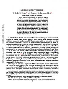
4. Case Study: Normalization and “Canonical Neural Computation” Our story begins in the late 1950’s with the discovery of simple cells in the primary visual cortex of the cat10 (Hubel & Wiesel 1962). These neurons were found to be extremely responsive to small, high contrast, bar-shaped stimuli placed at a particular location and orientation in the cat’s visual field. Hubel and Wiesel gave a qualitative description of simple cell response properties, and explained their elongated receptive field (RF) shape as due to the neurons’ feed-forward input from the lateral geniculate nucleus (LGN) (see Figure 1). In quantitative terms, Hubel and Wiesel’s account suggested that simple cells have linear response properties, i.e., that the 10

Strictly speaking, the term ‘V1’ only refers to primary visual cortex in primates, whereas ‘striate

cortex’ is appropriate for primary visual cortex of felines or primates. Below I do sometimes use ‘V1’ to refer to primary visual cortex of both kinds of animals, as is now quite common in the literature.

12

202

Forthcoming in Synthese sensation and perception

M. Chirimuuta

neuron’s receptive field could be mapped by observing its responses to small spots of light in the visual field, and that its response to any novel stimulus could be predicted from its receptive field map. This feed-forward, linear hypothesis was subjected to empirical scrutiny (using a variety of experimental animals) in the following decades and was found wanting in many respects.11 FIGURE 1: From Hubel and Wiesel (1962), the explanation of simple cell elongated receptive fields in terms of the arrangement of excitatory input from LGN cells which have circular receptive fields

A particularly important anomaly was the observation of cross orientation suppression. If the preferred stimulus of a simple cell (e.g. a small vertical bar) is superimposed a similar stimulus at mammalian a differentvisual orientation small horizontal bar), Figure 9.1. (a)with The main structures of the early system. (b)(e.g. From aHubel and Wiesel (1962), the explanation of simple is cellsignificantly elongated receptive fields in terms of theto its activity when response of the neuron reduced, compared rectangular arrangement of LGN input cells which have circular RFs (left). (c) From Hubel and Wiesel (1962), complexstimulus cells were classifi ed as having responses indifferent to the phasethe LGN inputs to preferred is presented alone (Bonds 1989). Since (black or white polarity) of the stimulus. This property was explained by their having simwould the(left). same in both stimulus conditions, this result cannot ple cell inputsneuron with various phase be tunings

the the the be

explained by Hubel and Wiesel’s account. A significant advance was made in 1992 while electrodes measured neuronal presented responses inthe the normalization cortex in termsmodel, of spikes per quantitative model of when David Heeger a new second. A crucial finding of Hubel and Wiesel (1959) was that neurons in the cat which account for findings such as cross visual cortexsimple respondcell wellresponse to moving properties or flashing bars of a could particular orientation, width, and location (see Hubel and Wiesel, 1998, for aidea historical overview orientation suppression. The basic of this modelofistheir that each simple cell has work, including the “accidental” discovery of elongated RFs). This suggested that excitatory inputand originating from nucleus the LGN, in contrast tolinear the neurons of the retina lateral geniculate (LGN)and whichin addition it receives had been found to haveinput circular RFsnearby (Kuffler, 1953), V1in RFs inhibitory from neurons the were visualelongated cortex. and The model is given by the

e Ch09.indd 202

following equation:

11

1/20/2009 12:20:32 AM

See AUTHOR for a more detailed review of these topics.

13


M. Chirimuuta

EQUATION 1.

Where Ēi is the normalised response (energy) of one simple cell, t is time, σ2 is a parameter which governs the contrast at which the model neuron will saturate and

Σ E determined by the sum of responses of all simple cells in a local population. The model is accompanied by a picture (Figure 2) which represents the pattern of excitatory and inhibitory inputs to V1 neurons (both simple and complex cells).

FIGURE 2

Findings such as cross orientation suppression are accounted for by the Σ E divisive normalisation term, which is thought to derive from a local inhibitory circuit in V1. That is, when a non-preferred stimulus (horizontal bar) is presented at the same time as the preferred stimulus (vertical bar), local neurons which are responsive to

14


M. Chirimuuta

the horizontal bar will be sending out a strong inhibitory signal, which will dampen the response of the one neuron to the vertical bar. The model has had countless applications within experimental and theoretical visual neuroscience (see Carandini & Heeger 2012 for review). In combination with the Gabor model of the receptive field (see section 5.2), normalization is an essential component of the “standard model” of primary visual cortex (Rust & Movshon 2005). According to the mechanistic framework, the normalization model would likely be classified as a “mechanism sketch” – that is, an incomplete description of the mechanism which correctly highlights some components of the mechanism, and describes some of their dynamics, but leaves many gaps and “filler terms” (Craver 2007:113, Kaplan & Craver 2011:609). In particular, the normalization model gives a quantitatively accurate prediction of cross orientation suppression, and numerous other phenomena (Heeger 1992), but its predictive ability is due to the Σ E term in Equation 1 which only describes the inhibitory mechanism in a very schematic way. It merely postulates that local neurons, those sensitive to a range of orientations and spatial frequencies (bar width), will send an inhibitory signals to each other, which combine to give the population suppressive effect, Σ E. It says nothing about the biophysical mechanism of inhibition – what neurotransmitters are involved, what its dynamics are, etc. . Kaplan and Craver take mechanism sketches to have limited explanatory value. While they do represent some features of the mechanism, as required by the 3M constraint, they stand in need of elaboration as more details of the underlying mechanism are discovered (MDB assumption). Mechanism sketches are way stations towards full blown explanatory models. To illustrate this view, it is worth mentioning Craver’s (2007:115) and Kaplan and Craver’s (2011:609) analysis of the HodgkinHuxley (HH) model of the action potential. They describe it as, at best, a mechanism sketch – because the details of how membrane voltage modulates ion conductivity were unknown until the 1970’s and are not described in the model. 12 Later 12

At worst, the HH model has been described by mechanist philosophers of neuroscience as a merely

phenomenal and not at all explanatory model (Craver 2008, Bogen 2008), or as a how-possibly model that has been falsified by later investigation and superseded by current how-actually models (Craver &

15


M. Chirimuuta

researchers discovered the voltage gated ion channels responsible for the conductivity changes and thereby improved on the original HH sketch. Kaplan (2011) presents three case studies of models in computational neuroscience that, according to his account, started out as predictively adequate but barely (or not at all) explanatory, and through discovery of underlying biophysical mechanisms have become truly explanatory. It might seem that the case study of the normalization model would conform to this pattern. For in 1994, Carandini and Heeger suggested a biophysical implementation of divisive normalization, shunting inhibition, and even showed that it is possible to derive Equation 1 from a fairly realistic model of membrane potential dynamics. This less sketchy model – which could be classified as a “how possibly” model within the mechanistic framework – is reported to be consistent with some extracellular physiological data. But, damningly, it is inconsistent with recent intracellular measurements (p.1335). In particular, it was observed that applying a GABA inhibition blocker to V1 does not abolish the cross orientation suppression effect, as would be predicted by the shunting inhibition mechanism. Carandini and Heeger (1994: 1335) speculate that an alternative mechanism for normalization could be one which affects the neuron’s gain (i.e. excitatory responsiveness), and evidence for this mechanism was presented in later publications (e.g. Carandini et al. 2002). Let us now fast forward to the present day. An interesting thing has happened to the neuroscients’ discussion of normalization, something not at all in alignment with the MDB assumption, or the mechanists’ preferred historical pattern of ever increasing elaboration of initial sketches. In a 2012 publication, Carandini and Heeger present the normalization model as a “canonical neural computation” (CNC). These are defined as “standard computational modules that apply the same fundamental operations in a variety of contexts” (p. 51). Other examples of CNC’s are linear filtering, recurrent amplification, associative learning, and exponentiation (a form of thresholding). They are presented as a toolbox of computational operations that the brain applies in a number of different sensory modalities and anatomical regions, and Kaplan 2011:355-358). See Weber (2005, 2008), Schaffner (2008), Levy (forthcoming), and Woodward (forthcoming) for contrary opinions.

16


M. Chirimuuta

which can be described at a higher level of abstraction from their biophysical implementation13. Carandini and Heeger review the diverse applications of the normalization model since 1992. Normalization models identical in form to Equation 1 have successfully been applied to an impressively wide range of neural systems: invertebrate olfaction; the retina (photoreceptors, bipolar cells, and retinal ganglion cells); neural network modelling of V1 development (e.g. Willmore et al. 2012); higher visual areas (MT, V4, IT); auditory cortex (A1); multi-sensory integration (area MST); visuo-motor control (area LIP); visual attention; and the model has also been used to model behavioural (psychophysical) data (AUTHOR). Although, the broad role of normalization is not thought to be the same in each of these systems, 14 the idea is that the same computation is performed in each case – that is, dividing the output response of a neuron by a term that relates to the average firing rate of nearby neurons. The third, and for our discussions most important characteristic of normalization as a CNC is that there is now good evidence that normalization is implemented by numerous different biophysical mechanisms, depending on the system in question. Both synaptic suppression and shunting inhibition are feasible implementations in certain brain regions, alongside noise and amplification mechanisms. In other words, normalization is multiply realized. Carandini and Heeger (2012) are now unambiguous in stating their view that there must be a conceptual distinction between understanding normalization as a CNC and more mechanistic considerations. For example, they claim, “[c]onceptually, it is useful to consider contrast normalization as separate from light adaptation, but mechanistically the two stages may overlap in bipolar cells” (p.52). Thus we see that 13

While the model-target distinction sometimes becomes blurred in the neuroscientific literature –

sometimes a computation is talked about as if it is just a model, and sometimes it is treated as a function belonging to the neural circuit itself – it is worth delineating it at this point. CNC’s are computations performed by neurons and circuits in the brain. Thus the normalization model, e.g. Equation 1, is a representation of the neural computations. 14

Amongst the many proposed functions of normalization are: maximizing sensitivity of sensory

neurons; sharpening the tuning of sensory neurons; decoding distributed neural representations; discriminating amongst stimuli; computing a winner-take-all pooling rule; and redundancy reduction.

17


M. Chirimuuta

Carandini and Heeger endorse a “distinctness of computation” thesis: the idea that there can be principled reasons for analyzing neural systems computationally rather than mechanistically. I do not call the claim an “autonomy of computation” thesis because they are not proposing that CNC’s are fully independent of biophysical implementation, or that CNC’s can best be studied in full isolation from mechanistic considerations. This distinctness thesis of course assumes that computational explanations do have a sui generis form. Thus I interpret Carandini and Heeger as endorsing modified versions of Kaplan’s C1 (autonomy) and C3 (distinctness) theses. Before concluding the normalization story, I should mention that elsewhere Carandini (2012) has advocated the CNC project as an important step toward linking our knowledge of neural anatomy and physiology (i.e. mechanism) to behavior and cognition. As Carandini and Heeger (2012:61) write, “[i]dentifying and characterizing more modular computations of this kind will provide a toolbox for developing a principled understanding of brain function.”15 In other words, the idea is that a dedicated computational analysis of neural circuitry will be a route to better explanations of the brain and of the brain’s contribution to behaviour. For example, in a report from a 2009 workshop on CNC’s Angelaki (et al. 2009) write that, “These models have led to important simplifying insights into the relationship between neural computations and behavior. …for example … that a seemingly heterogeneous variety of forms of attentional modulation can be understood as resulting from a simple model of contrast gain control.” Elsewhere in the same report Caddick (et al. 2009) make the comparison between the search for CNC’s and the discovery of “secondary structure” in molecular. The “primary structure” of a protein is its sequence of base pairs, whereas the “secondary structure” characterises domains, protein substructures that are rearranged, like lego bricks, in different proteins to build various functional units. As Caddick (et al. 2009) write, “ “secondary structure” has been identified as a fruitful 15

Incidentally, Weiskopf (2011a:249) presents a similar idea when he writes, “The interesting

functionally defined categories, then, constitute recurrent building blocks of cognitive systems. They explain the possession of various capacities of those systems without reference to specific realizing structures.” Though he does not focus here on non-mechanistic explanation.

18


M. Chirimuuta

level of abstraction to understand proteins, the level that provides the appropriate modules.” They propose that the discovery of analogous modules in neuroscience – canonical neural computations – is our best bet at tackling the “staggering complexity” of the brain. Let us now summarise the main points of the case study. We have traced the varying fortunes of the normalization model from its early beginnings as a sketch-like explanation of nonlinear behaviour of V1 simple cells, to its troubled adolescence as a how-possibly mechanistic model. The reader may have been saddened as it failed to mature into a fully fledged how-actually model. Yet in the end we have witnessed an interesting turn of events: the model has been reinvented as a canonical neural computation. Along the way we have seen that the mechanists’ 3M requirement and MDB assumption sit oddly (to put it mildly) with the new interpretation and status of the normalization model. For Carandini and Heeger (2012) no longer think that we should interpret the normalization model mechanistically, as describing components and dynamics of a neural mechanism. Instead, they focus on the informationprocessing principles encapsulated by the model. Furthermore, any digging down to more mechanistic detail would simply lead us to miss the presence of CNC’s entirely, because of their many different realizations. More details are certainly not for the better, in this case. And because undetailed CNC models like normalization are not way-stations to more detailed mechanistic models, I urge that they be considered as a type of minimal model. The representational ideal (Weisberg 2007) of minimal models is not that of fidelity to the fine-detail of nature. In the next section I will compare CNC’s to other examples of minimal models and outline the explanatory form associated with CNC’s.

5. Information, Explanation, and I-Minimal Models What is explanation? Not an easy question. If one reads the literature on the normalization model one finds the word “explain” being used in various ways. For example, it is said that the model explains nonlinearity of V1 in the sense that it fits the existing data (e.g. on non-specific suppression) and is expected to do well in

19


M. Chirimuuta

predicting data from new experiments. On other occasions, the model is said to explain in the sense of providing a unifying framework for past and future empirical investigation. Both of these senses are alluded to by Heeger (1992:192): “The new model explains much of the existing experimental data on striate cell responses, and provides a theoretical framework in which to carry out future research on striate cortical function” Chemero and Silberstein (2008) take prediction and unification to be sufficient for explanation, and argue on those grounds that non-mechanistic, dynamical systems models in psychology and cognitive neuroscience are explanatory. This is the claim contested by Kaplan and Craver (2011). So while I am all for taking the scientists’ own notions of explanation seriously, and am also in favour of pluralism about explanation that accommodates unificationist criteria where these may apply (Khalifa 2012), these are not positions I will aim to defend here. Instead, I will show that one common pattern of non-mechanistic explanation is indeed explanatory by one of the mechanists’ core criteria (see Kaplan 2011:354) – namely, the ability to address “whatif-things-had-been-different questions” or “w-questions” (Woodward 2003). This is the efficient coding pattern of explanation. In order best to describe this distinctive explanatory type, I will return to the notion of minimal models introduced above, and contrast CNC’s with the other kinds of minimal models discussed in the philosophy of science literature. 5.1 I-Minimal Models A-minimal models were defined in Section 3 as those which provide a pared down account of the causal factors that give rise to the explanandum phenomenon. For example, Woodward (forthcoming) and Levy (forthcoming) describe the HodgkinHuxley (1952) model of the action potential in this way. If one takes the voltage-time profile of the action potential as the primary explanandum, then the HH model explains this in terms of voltage sensitive conductivity changes in the neural membrane. It describes how the membrane’s changing conductivity to potassium and sodium ions generates the action potential profile, but does not describe the biophysical mechanism for conductivity changes, i.e. the voltage gated ion channels which were discovered only later. The model is said to represent the action potential mechanism in a highly abstract way. As Levy and Woodward and Schaffner

20


M. Chirimuuta

(2008) point out, one of the advantages of an A-minimal model over a fully detailed mechanistic model is that it has greater generality – it can be used to model the action potentials in a range of neuron types in various different species, where biomechanics are quite dissimilar. Like a mechanism sketch, an A-minimal model can still be thought of mapping onto mechanism components in a coarse-grained way; but it should not be thought of as an incomplete model, standing in need of subsequent addition of explanatory detail. As indicated above when I discussed one possible interpretation of Heeger’s (1992) normalisation model as a mechanism sketch, such CNC’s could similarly be characterised as A-minimal models. For example, one could take the Σ E term to be representing the causal mechanism for neuronal inhibition in a very abstract manner, in the same way that the HH model gives a very abstract representation of the causal operation of ion channels. However, I caution that any attempt at assimilation of CNC’s into the class of causal-mechanical models, even the most minimal ones, would make one oblivious to the defining characteristics of CNC’s. The central point of Carandini and Heeger’s (2012) account is that CNC’s do not attempt to describe mechanisms – which vary significantly from one instance of a CNC to another, even when described in a very abstract manner – but rather a universal feature of the different systems to which the one CNC model, like normalisation, will apply. This feature is a computation. They write, for example, that “it is unlikely that a single mechanistic explanation [for normalization phenomena] will hold across all systems and species: what seems to be common is not necessarily the biophysical mechanism but rather the computation.” It is worth noting that the distinction between computation and mechanism is rather commonplace in neuroscience. For example, Sejnowski et al. (1988:1300) write that, “mechanical and causal explanations of chemical and electrical signals in the brain are different from computational explanations. The chief difference is that a computational explanation refers to the information content of the physical signals and how they are used to accomplish a task”. So rather than wade into the vast literature which concerns definitions of computation16, I suggest we instead examine the specific ways in which 16

For starters, see Piccinini (2006), Piccinini and Scarantino (2010).

21


M. Chirimuuta

Carandini and Heeger’s models can be said to describe computations rather than mechanisms. The term ‘normalization’ has a variety of meanings in mathematics and engineering, which convey the idea of a function that brings values of a variable into a pre-defined normal range. Heeger (1992) transferred this idea to the neuroscience context, where the contrast normalization equation, in essence, models how the activity levels of simple cells are continually brought down to a normal operating range via a kind of negative feedback operation. Carandini and Heeger (2012) review evidence that an equivalent normalization process occurs in a variety of sensory and nonsensory brain areas. My key claim is that the use of the term ‘normalization’ in neuroscience retains much of its original mathematical-engineering sense. It indicates a mathematical operation – a computation – not a biological mechanism. These neuroscientists are making the commonplace assumption that neurons in the brain can be said to compute mathematical functions, which can be characterised by formalisms like Equation 1; moreover, that these computations are the function of the neural system, such that if you want to know what the system is for, you have to say what it computes17. To take another example of a CNC, the term ‘linear filter’ originates in engineering to describe a process which generates an output signal by performing a linear operation on the input signal (e.g. a bandpass filter reproduces the signal over a certain frequency band and removes other frequencies). In saying that neurons in primary sensory areas are linear filters, the claim is that they perform this kind of mathematical analysis. Because of Carandini and Heeger’s emphasis on the universal characteristics of CNC’s, and their proposal that CNC’s should not be understood mechanistically, it is interesting to compare them with Batterman’s (2002, 2009) account of non-causalmechanical models in physics – called B-minimal models above. The important shared feature of B-minimal models and CNC’s is that they define a universality class. In the case of the normalization model, this is the group of neural circuits that can all be described by Equation 1. To take one of Batterman’s (2002:37 ff.) examples, this is 17

See textbooks such as Churchland and Sejnowski (1992), Koch (1998), Dayan and Abbott (2001),

Trappenberg (2010), Sterratt et al. (2011).

22


M. Chirimuuta

the group of all materials whose phase transitions near a critical point can be characterised by the same dimensionless number, the “critical exponent”. Batterman (2002:13) describes two general characteristics of universality: 1. “The details of the system (those details that would feature in a complete causal-mechanical explanation of the system’s behavior) are largely irrelevant for describing the behavior of interest. 2. Many different systems with completely different “micro” details will exhibit identical behavior.” These characteristics certainly apply to canonical neural computations.18 An important difference between B-minimal models and CNC’s become apparent if we focus on the kinds of scientific accounts given to explain the universal behaviour itself. In the physics examples discussed by Batterman, the mathematical procedures employed in deriving the models themselves explain why micro details of the system ought to be largely irrelevant when modelling the critical behaviour. Batterman (2002) calls this “asymptotic explanation”. No such formal niceties are available in neuroscience. Instead, the explanation of universality refers to the computational function of the modelled behaviour – that is, the computational problem that the modelled system is able to solve. This is how Carandini and Heeger (2012:60) put the matter: “Why is normalization so widespread? A tempting answer would be to see it as a natural outcome of a very common mechanism or network; a canonical neural circuit19. However, there seem to be many circuits and mechanisms underlying normalization and they are not necessarily the same across species and systems. Consequently, we propose that the answer has to do with computation, not mechanism.” In other words, the presence of equivalent computational needs in different systems means they will converge on the same CNC’s. For instance, Heeger (1992) proposed that contrast normalization in primary visual cortex had an important role to play in 18

In a sense A-minimal models can also be said to define a universality class. E.g. all those neuron’s

whose action potential’s can be described by HH model. Here, explanation of the universality is that the model captures the shared, essential difference makers across all of these different neurons. 19

Anderson’s (2007) notion of a “working” would be an example of this hypothetical kind of circuit.

23


M. Chirimuuta

maintaining the tuning specificity of simple cells to a small range of stimulus orientations, regardless of increasing overall stimulus contrast20. Since maintenance of fixed stimulus selectivity is required for reliable sensory coding in other modalities, it is not at all surprising that normalization has been observed in nonvisual areas, and in invertebrates, even though the mechanistic implementation must be different. Thus, if our question is, why should so many systems exhibit behaviour described by normalization equation? The general answer is, because for many instances of neural processing individual neurons are able to transmit more information if their firing rate is suppressed by the population average firing rate. If “suppressed” still sounds to your ears like yet more elliptical mechanistic explanation, please bear with me as a I proceed to describe this explanatory framework and supply further examples. In order to emphasize the difference between CNC’s and the two other kinds of minimal models discussed above, I will baptize a new model type, I-minimal model, where “I” stands both for “interpretative” and “informational”. With a nod to Dayan and Abbott’s (2001:xiii) gloss on interpretative models, I define I-minimal models as: Models which ignore biophysical specifics in order to describe the information processing capacity of a neuron or neuronal population. They figure in computational or information-theoretic explanations of why the neurons should behave in ways described by the model. Such explanations can be made precise and quantitative by reference to efficient coding principles. This idea can be illustrated with the example of redundancy reduction. As Attneave (1954) observed, natural visual stimuli are highly redundant. Because of edges, repeated textures, and other frequently occurring features, it is often possible to predict what the next pixel in an image will be from knowledge of the previous one. An inefficient code of a natural image is one which specifies each pixel value (e.g. a bitmap); whereas a more efficient code is one which exploits the natural redundancies and can convey the same information about structure but with a shorter signal length (e.g. a jpeg). Barlow (1961) proposed that one of the functions 20

Note that Hubel and Wiesel’s hierarchical feedforward model predicts that for high contrast stimuli

simple cells will be less selective about orientation, in conflict with empirical observations.

24


M. Chirimuuta

of early visual processing is to minimise the transmission of redundant information and therefore to represent visual information in a more efficient manner. This can be done if the responses of neurons in the early visual system are decorrelated – made maximally independent from one another. Simulations by Schwartz and Simoncelli (2001) showed that normalisation is a way to achieve decorrelated signals for neurons in the early visual and auditory system. Hence they provided an efficient coding explanation for the response properties of these neurons, in terms of the computational value of normalisation. 21 We can now come to appreciate the distinctive explanatory value of I-minimal models. They figure prominently in explanations of why a particular neural system exhibits a particular empirically observed behaviour, by referring to its computational function. For example, when cross orientation suppression was first observed it was a baffling, anomalous finding. The 1992 contrast normalization model was able to unify an impressive amount of anomalous data and by showing that these results could be predicted by one simple model of neuronal processing in V1. Furthermore, by considering the functional importance of normalization – e.g. in retaining orientation tuning specificity, or redundancy reduction – it could be shown why it is expedient of sensory areas like V1 to implement normalization. These efficient coding explanations account for observed properties of neural circuits in terms of the computational advantages of that particular arrangement of neurons. Note that the appeal to coding principles like redundancy reduction does not involve decomposition of any mechanism thought to underlie the behaviour in question. 21

Similarly, Olsen et al. (2010) have studied normalization in the olfactory system of drosophila.

Quoting Simoncelli (2003), they present a two part efficient coding hypothesis, stating “(1) each neuron should use its dynamic range uniformly, and (2) responses of different neurons should be independent” (p. 295). They manipulate parameters of normalization in a computer simulation of the fly’s olfactory system and show that normalization decorrelates neuronal responses, as required by (2), and that a similar gain control transformation boosts weak responses to select stimuli, as required by (1). They also show that the simulation findings fit with the empirical observations of decorrelation in the fly’s area PN. It should be noted that the simulation in which the normalization equation is embedded is highly abstract. It is not intended as a realistic, biophysical simulation of these neural systems. Rather, each neuron is modelled by a single number which represents its response to the olfactory stimulus, and the entire population model only simulates 24 out of 50 neuronal types that have been found in the target brain area.

25


M. Chirimuuta

Rather, it takes an observed behaviour and formulates an explanatory hypothesis about its functional utility22.

5.2 Another Look at Receptive Field Models A final example -- the Gabor model of V1 receptive fields -- will reinforce the point about the distinctness and significance of computational explanation in neuroscience, and will illustrate an explanatory strategy that is common in the field. Within the CNC framework the Gabor model would be classified as a kind of linear filter. Unlike the normalisation model, the Gabor model cannot be interpreted as a mechanism sketch or A-minimal model. Hence it breaks fully with the 3M criterion for explanatory success, and would be classified by Kaplan (2011) and Kaplan and Craver (2011) as a merely phenomenal, data-fitting model. In this section I will show that the Gabor model does figure in genuine computational explanations, ones which address Woodward’s (2003) w-questions. FIGURE 3

22

Rieke et al.’s (1999) Spikes is a classic text on efficient coding and the application of information

theory to neuroscience. Other examples of efficient coding explanation are: Laughlin (1981), Srinivasan et al., 1982; Atick and Redlich, 1992; van Hateren, 1992; Rieke et al., 1995; Dan et al., 1996; Olshausen and Field, 1996; Baddeley et al., 1997; Bell and Sejnowski, 1997; Machens et al., 2001; Schwartz and Simoncelli, 2001; Vincent et al. 2005; Chechik et al., 2006; Graham et al., 2006; Smith and Lewicki, 2006; Borghuis et al., 2008; Liu et al., 2009; Doi et al. 2012.

26


M. Chirimuuta

EQUATION 2 g(x,y) = K exp [- ½ (x2g/a2+y2/b2)] x cos [-2π (U0x + V0y) – P] Figure 3 is a graphical representation of a Gabor function, placed beside a map of a simple cell receptive field of the sort presented by Hubel and Wiesel (1962). Equation 2 gives the real (observable) part of a generalized 2D Gabor filter (Jones & Palmer 1987:1236). a2 and b2 are variance in the x and y direction, respectively. x, y, U0 and V0 are spatial coordinates, K is a scale factor, and P can be interpreted as the relative spatial phase angle of the modulation term. Note that no parameters of Equation 2 can be thought of as referring to parts of neurons or circuits, as might be argued in interpreting the normalisation model (Equation 1). Alongside contrast normalisation, the Gabor model of the simple cell receptive field is an important element of the standard model of V1 (Rust & Movshon 2005). The Gabor function is a product of a sinusoid with a Gaussian envelope, giving a local sinusoidal modulation (Gabor 1946). The Model can be used to give a fairly accurate fit to data on V1 neurons’ responses to simple artificial stimuli and more complex natural scenes23. Kaplan (2011:359) presents a similar model – the difference of Gaussians model of retinal ganglion cell RF’s – as an example of a phenomenalmodel, one which fits the data on the visual responses or neurons without offering any explanation of them. On his view, only non-phenomenological mechanistic models which show how neuronal circuits are arranged to give neurons their characteristic RF shape, are genuinely explanatory. Thus I presume that the Gabor model, which is in effect a black box model, would be subject to an equivalent analysis by Kaplan. Nevertheless, there are at least two ways in which the Gabor model has been employed in explanations of V1 neuronal response properties. The explanandum is the following: why do V1 simple cells have elongated receptive fields of the sort that can be fit by Equation 2?24 The first explanation notes that the Gabor function originated 23

See Olshausen and Field (2006) and AUTHOR on limitations of the model.

24

And see Dayan and Abbott (2001: 135-141) and Doi et al. (2012) for efficient coding explanations of

retinal ganglion cell RF’s.

27


M. Chirimuuta

in signal engineering because it was found to have the interesting informationtheoretic property of minimising joint uncertainty over time and frequency of signal (Gabor-Heisenberg-Weyl uncertainty). In its application to visual space, it can be said to minimise joint uncertainty over location and spatial frequency of a stimulus. Thus a viable explanation is because this minimises Gabor-Heisenberg-Weyl uncertainty, and thus is an efficient way of coding visual information. Indeed, this proposal was made by Daugman (1985) in one of the first papers that introduced the Gabor function to visual neuroscience. As we have seen, this explanatory strategy is formalised in neuroscience by use of information theory. The general strategy is to work from information-theoretic first principles to build a model of a hypothetical system which would maximise information transmission of the sort required by the brain area in question. Then one sees how the hypothetical optimal and real system line up with respect to neuronal response properties and other features. If there are similarities in the properties compared, we have an explanation of why the brain area has those properties. Note that no strong adaptationist assumption lurks behind this kind of efficient coding explanation; rather, it is a “methodological adaptationism” of the sort described by Godfrey-Smith (2001). It is not assumed that V1’s actual response properties must be optimal, but simply that it is explanatorily relevant to compare properties of the actual system to hypothetical optimal systems. Since it is well recognised that it is metabolically costly to sustain neural tissue, at high firing rates (Lennie 2003), it is acceptable to assume that the “design” of the nervous system is constrained by metabolic factors such that, where possible, neurons and circuits are arranged to ensure that each neuron transmits the most information for the least energy investment (Laughlin 2001). Thus one background assumption is that there is some set of processes at work -- in evolutionary, developmental, and even shortterm time frames (Wainwright et al. 2001: 410) -- which have some tendency to optimize solutions to coding problems. The specification of these processes is outside the remit of the efficient coding explanation. But such explanations do imply that if the problem were to vary in such a way that it had a different optimal solution, then observed properties of the actual system would also vary.

28


M. Chirimuuta

Thus it follows that efficient coding explanations delineate a set of counterfactual dependencies between input to the system (e.g. sensory information) and/or system requirements (e.g. task for which information is needed) and the computational properties of the system. For example, if one imagines that the V1 code had no requirement for spatial frequency information, then one would predict that the receptive fields would be different such that they minimised uncertainty about position alone. So the uncertainty-minimising explanation of V1 receptive field properties turns out to address “what-if-things-had-been-different questions” or “wquestions” (Woodward 2003). The dependency relationship between sensory information and normalisation has been explored empirically and computationally and been shown to support interventions. Wainwright et al. (2001) show that the specific decorrelation strategy employed by early visual codes is dependent on the kinds of statistical dependencies present in natural images, and that changes in decorrelation strategy can occur in a short-term time frame, as adaptational effects. Thus this efficient coding explanation turns out to be a causal one according to Woodward’s (2003) interventionist theory, which is widely accepted in the mechanist philosophy of neuroscience literature (e.g. Craver 2007, Kaplan & Craver 2011). It is worth making the comparison between the kind of causal explanation that I am describing and Mayr’s (1961) notion of ultimate causal explanation, as distinct from proximal causal explanations. Typically, the proximal explanation describes the mechanism by which a particular feature or behaviour of an organism comes about. To take the example of V1 receptive fields, the proximal explanation for their properties would be in terms of the particular excitatory and inhibitory inputs the neurons receive, and their distinctive biophysical makeup – dendrite configuration, ion channels, etc.. Note that this is the kind of explanation that Kaplan (2011) takes to be the only possible explanation of RF’s in the retina. But that is to assume that there is just one kind of causal story to be told about a system (cf. Piccinini and Craver 2011). Mayr’s view was that ultimate causal explanations which refer to evolutionary principles are an important supplement to reductive, proximal accounts (Beatty 1994). Ultimate explanations refer to causal factors that were significant in the evolutionary, and in our case developmental or recent stimulus history of the

29


M. Chirimuuta

organism, and have led to the behavior or feature now observed. Yet, they do not describe a causal path leading to any current instantiation of the behavior or feature and so can easily be distinguished from local mechanistic explanations.

6. Lessons, Levels and Perspectives The main thrust of this paper has been to endorse a claim for the distinctness of computational explanation in neuroscience. While Kaplan (2011) considered only Cummins’ (1983) version of the distinctness thesis (C3), I have shown that many computational

neuroscientists

clearly

distinguish

between

mechanistic

and

computational explanations, and that this distinction is characterised by efficient coding explanations, rather than generic functional explanations. The efficient coding explanations described above are non-mechanistic in that they break with Kaplan’s 3M and MDB criteria. Nonetheless, they are still causal explanations according to Woodward’s interventionist theory. The kinds of efficient coding explanation I have described do align closely with patterns of non-mechanistic explanation in biology, as was evident in the comparison with Mayr’s concept of ultimate explanation. For example, many philosophers of biology have argued, teleological explanation is an important supplement to mechanistic approaches (see Allen et al. 1998). So if a proponent of the mechanist approach to computational neuroscience chose to resist my argument by denying the explanatory status of I-minimal models, she risks committing herself to the claim that numerous non-mechanistic models in biology are non-explanatory. In effect, the mechanists who hold that computational explanation in neuroscience and cognitive science is just a form of mechanistic explanation are advocating explanatory monism. In contrast, I urge the reader to consider a kind of explanatory pluralism whereby the same system in neuroscience can be represented and modelled in a variety of different ways, depending on the particular purposes of the investigation. These different perspectives on a system need not be in competition and may well be complementary (Mitchell 2002, Giere 2006). Both computational

30


M. Chirimuuta

and mechanistic models have a place25. In order to build models of V1 for decoding fMRI data the computational perspective is primary.

The challenge here is to

understand the features of V1 as an information processing system in order to “unlock the neural code”, and not coincidentally, non-mechanistic models like the Gabor filter are important tools for this task (Nishimoto et al. 2011). To say the brain is a computational system is just to have a particular modelling perspective on the brain (cf. Shagrir 2010a). If the goal of research is to develop pharmacological interventions to cure neural diseases, mechanistic models are more valuable. And arguably both maximalist and minimalist projects in neuroscience have something to offer. As Zucker (2006) urges, “while local [i.e. small-scale, detailed and realistic] models are important, it is as important to explore the other way around; that is, to find the right types of abstraction for characterizing the cortical machine.” (p. 217; cf. Salinas 2008). One consequence of the perspectival pluralism just sketched here is that the issue of levels in neuroscience is divorced from consideration of scale, size, and mereology in general. While Marr’s (1982) tripartite division of levels is often interpreted as mapping onto different scales, which themselves track the neuroscience-psychology boundary

26

– the implementation (mechanistic) level being associated with

neuroscience of single neurons or small circuits and the algorithmic and computational levels being associated with psychology of the whole organism – we have seen that this hierarchy does not track the computation-mechanism distinction within neuroscience. Single neurons may be treated both as intricate biological mechanisms or as miniature computational systems (Koch 1998). Another lesson to be learned is that the thesis of autonomy (C1) should be rehabilitated rather than fully rejected. We may all agree that Johnson-Laird and Fodor were wrong to think that a computational science of the mind could come to fruition without regard to any developments in neurophysiology. But as Carandini and Heeger (2012) have shown, some interesting computational properties of neural 25

I would consider the dynamical systems approach to be another distinct perspective (e.g. Buzsáki

2006, Chemero & Silberstein 2008, Izihikevich 2010), though there is not time to discuss this here. 26

This is Kaplan’s (2011) interpretation, but see Shagrir (2010b) for an alternative reading of Marr.

31


M. Chirimuuta

systems do appear to be partially independent of their mechanistic realizers. And there is nothing mysterious about this. It is useful to consider the claim for the multiple realizability of neural computations as simply a claim about where the interesting regularities show up in neural systems (Carandini 2012). That is, if one looks at the brain purely from the mechanistic perspective one sees a dauntingly heterogeneous array of biological to-ings and fro-ings, which often have no obvious connection to cognition or behaviour. Yet if one examines the brain from the computational perspective one sees that various mechanisms have a shared computational function that can, in turn, be related to cognition and behaviour. To conclude, there has been an expansionist current to recent attempts to bring mechanistic philosophy of neuroscience into the new territory of computational, cognitive and systems research. As Kaplan and Craver (2011:611) write: Given that one expects cognitive mechanisms ultimately to be composed of lower-level mechanisms of this [biophysical] sort, in a manner that might be illustrated in a telescoping hierarchy of mechanisms and their components, it would be most tidy and parsimonious if the ideal of mechanistic explanation were to be extended from top to bottom across all fields in neuroscience. Our intended opponent suggests that cognitive and systems neuroscientists should abandon this set of explanatory ideals in favor of an alternative form of explanation. This suggestion, if it is to have content, should come with principled reasons for abandoning those ideals of explanation. One principled reason why we are likely to need multiple perspectives is, simply put, because the brain is complex (cf. Mitchell 2002, 2009). Cognitive neuroscience has to contend with systems of unparalleled complexity, even by the impressive standards of the rest of biology. There are approximately 86 billion neurons in the brain, with trillions of synaptic connections between them (Azevedo et al. 2009). When faced with such challenges, the standard scientific response is to simplify the problem space: restrict attention to a limited range of causally significant components and forget about trying to model all of them; leave out most of descriptive details of these selected components, and approximately describe their dominant behaviours; search for some mathematically convenient equations to describe the system’s internal dynamics, even at the expense of precise data-fitting. Needless to say, these

32


M. Chirimuuta

are the techniques of minimal modelling described in the most general terms. If one is tempted to reply that these methods devised to handle complexity are “merely pragmatic” concerns and not of central interest in the philosophy of science, I suggest that a heavy dose of reality would be most helpful at this stage of the debate; for what I am describing is a prominent feature of the scientific method and thus should be a central concern for philosophers of science. Mathematical physicist G. I. Barenblatt (1996), advises that, “the crucial step in any field of research is to establish what is the minimum amount of information that we actually require about the phenomenon being studied” (quoted in Batterman 2002). Not coincidentally, the same sentiment is echoed in the literature on canonical neural computation: “the computer analogy illustrates a general rule in science, which is to seek an appropriate level of description” (Carandini 2012:507). Acknowledgements I would like to thank participants in the Pitt ‘Representations, Perspectives, Pluralism’ seminar, in particular my co-teachers Sandra Mitchell and Jim Bogen, for early discussions of this material. I am also grateful to audience members at the Pitt Center for Philosophy of Science where this paper was originally presented. I am indebted to Jim Bogen, Carrie Figdor, Arnon Levy, Peter Machamer, Collin Rice and James Woodward for comments on the manuscript, and also to the anonymous referees for many helpful suggestions. Finally, I would like to thank David Heeger for permission to use Figure 2.

References Allen, C., Bekoff, M., & Lauder, G. (1998). Nature's Purposes: Analyses of Function and Design in Biology. Cambridge, MA: Bradford Books. Anderson, M.L. (2010). Neural reuse: A fundamental organizational principle of the brain. Behavioral and Brain Sciences 33, 245–313. Angelaki, D., Caddick, S., Movshon, T., Reynolds, J., Rust, N., Shamma, S., Solomon, S., & Yokoyama., C. (2009). Physiology: Systems. In Heeger et al. (eds.) Canonical

Neural

Computation:

A

33

Summary

and

a

Roadmap.


M. Chirimuuta

http://www.theswartzfoundation.org/docs/Canonical-Neural-Computation-April2009.pdf Atick, J.J., & Redlich, A.N. (1992). What does the retina know about natural scenes? Neural Comput 4, 196 –210. Attneave, F. (1954). Some informational aspects of visual perception. Psych. Rev., 61, 183–193. Azevedo, F.A.C., Carvalho, L.R.B., Grinberg, L.T., Farfel, J.M., Ferretti, R.E.L., Leite, R.E.P., Filho, W.J., Lent, R., & Herculano-Houzel, S. (2009). Equal Numbers of Neuronal and Nonneuronal Cells Make the Human Brain an Isometrically Scaled-Up Primate Brain. Journal of Comparative Neurology, 513, 532–541. Baddeley, R., Abbott, L.F., Booth, M.J.A., Sengpiel, F., Freeman, T., Wakeman, E.A., & Rolls, E.T. (1997). Responses of neurons in primary and inferior temporal visual cortices to natural scenes. Proc Biol Sci, 264, 1775–1783. Barenblatt, G.I. (1996). Scaling, Self-similarity, and Intermediate Asymptotics. Cambridge: Cambridge University Press. Barlow, H.B. (1961). Possible principles underlying the transformation of sensory messages. In: W.A. Rosenblith (Ed.) Sensory Communication. Cambridge, MA: MIT Press. Batterman, R. (2002). The Devil in the Details. Oxford: Oxford University Press. Batterman, R. (2009). Idealization and modeling. Synthese, 169, 427–446. Beatty, J. (1994). The Proximate/Ultimate Distinction in the Multiple Careers of Ernst Mayr. Biology and Philosophy, 9, 333-356. Bechtel, W. (2008). Mental Mechanisms: Philosophical Perspectives on Cognitive Neu- roscience. London: Routledge. Bechtel, W., & Mundale, J. (1999). Multiple realizability revisited: Linking cognitive and neural states. Philosophy of Science, 66, 175–207. Bechtel, W., & Richardson, R.C. (1993). Discovering Complexity. Princeton, NJ: Princeton University Press. Bell, A.J., & Sejnowski, T.J. (1997). The independent components of natural scenes are edge filters. Vision Research, 37, 3327–3338. Bogen, J. (2008). The Hodgkin-Huxley Equations and the Concrete Model: Comments on Craver, Schaffner, and Weber. Philosophy of Science, 75, 1034– 1046.

34


M. Chirimuuta

Bogen, J., & Machamer, P. (2010). Mechanistic Information and Causal Continuity. In: P. McKay, F.R. Illari, & J. Williamson (Eds.), Causality in the Sciences (pp. 845-864): Oxford University Press. Bonds, A.B. (1989). Role of inhibition in the specification of orientation selectivity of cells in the cat striate cortex. Visual Neuroscience, 2, 41–55. Borghuis, B.G., Ratliff, C.P., Smith, R.G., Sterling, P., & Balasubramanian, V. (2008). Design of a neuronal array. J Neurosci 28, 3178 –3189. Brandon, R.N. (1981). Biological teleolog: questions and explanations. Stud. Hst. Phil. Sci., 12 (2), 91-105. Buzsáki , G. (2006). Rhythms of the Brain. Oxford: Oxford University Press. Caddick, S., Carandini, M., Hausser, M., Martin, K., Priebe, N., Reynolds, J., Scanziani, M., Wiedemann, C., Wilson, R., & Yokoyama, C. (2009). Physiology: Mechanisms. In Heeger et al. (eds) Canonical Neural Computation: A Summary and a

Roadmap.

http://www.theswartzfoundation.org/docs/Canonical-Neural-

Computation-April-2009.pdf Carandini, M. (2012). From circuits to behavior: a bridge too far? Nature, 15 (4), 507509. Carandini, M., Demb, J.B., Mante, V., Tolhurst, D.J., Dan, Y., Olshausen, B.A., Gallant, J.L., & Rust, N.C. (2005). Do We Know What the Early Visual System Does? Journal of Neuroscience, 25 (46), 10577–10597. Carandini, M., & Heeger, D.J. (1994). Summation and division by neurons in primate visual cortex. Science, 264, 1333–1336. Carandini, M., & Heeger, D.J. (2012). Normalization as a canonical neural computation. Nature Reviews Neuroscience, 13, 51-62. Carandini, M., Heeger, D.J., & Senn, W. (2002). A Synaptic Explanation of Suppression in Visual Cortex. Journal of Neuroscience, 22 (22), 10053–10065. Chechik, G., Anderson, M.J., Bar-Yosef, O., Young, E.D., Tishby, N., & Nelken, I. (2006). Reduction of information redundancy in the ascending auditory pathway. Neuron, 51, 359 –368. Chemero, A., & Silberstein, M. (2008). After the Philosophy of Mind: Replacing Scholasticism with Science. Philosophy of Science, 75, 1–27. Churchland, P.S., & Sejnowski, T.J. (1992). The Computational Brain. Cambridge, MA: MIT Press. Craver, C.F. (2006). When Mechanistic Models Explain. Synthese, 153, 355–376.

35


M. Chirimuuta

Craver, C.F. (2007). Explaining the Brain. Oxford: Oxford University Press. Craver, C.F. (2008). Physical Law and Mechanistic Explanation in the Hodgkin and Huxley Model of the Action Potential. Philosophy of Science, 1022–1033. Craver, C.F., & Darden, L. (2001). Discovering Mechanisms in Neurobiology: The Case of Spatial Memory. In: P. Machamer, R. Grush, & P.McLaughlin (Eds.), Theory and Method in the Neurosciences. Pittsburgh: University of Pittsburgh Press. Cummins, R. (1983). The nature of psychological explanation. Cambridge, MA: Bradford/MIT Press. D.H., H., & N., W.J. (1962). Receptive fields, binocular interaction and functional architecture in the cat’s visual cortex. Journal of Physiology, 160, 106 –154. Dan, Y., Atick, J.J., & Reid, R.C. (1996). Efficient coding of natural scenes in the lateral geniculate nucleus: experimental test of a computational theory. J Neurosci 16, 3351–3362. Daugman, J.G. (1985). Uncertainty relation for resolution in space, spatial frequency, and orientation optimized by two-dimensional visual cortical filters. J. Opt. Soc. Am. A, 2 (7), 1160-1169. Dayan, P., & Abbott, L.F. (2001). Theoretical Neuroscience: Computational and Mathematical Modeling of Neural Systems. Cambridge, MA: MIT Press. Doi, E., Gautier, J.J., Field, G.D., Shlens, J., Sher, A., Greschner, M., Machado, T.A., Jepson, L.H., Mathieson, K., Gunning, D.E., Litke, A.M., Paninski, L., Chichilnisky, E.J., & Simoncelli, E.P. (2012). Efficient Coding of Spatial Information in the Primate Retina. Journal of Neuroscience, 32 (46), 16256 –16264. Fodor, J.A. (1975). The language of thought. Cambridge, MA: Harvard University Press. Gabor, D. (1946). Theory of communication. Journal of the Institution of Electrical Engineers, 93, 429-459. Gazzaniga, M.S., Mangun, G., & Ivry, R. (1998). Cognitive Neuroscience: The Biology of the Mind. New York: W. W. Norton. Giere, R. (2006). Scientific Perspectivism. Chicago: Chicago University Press. Godfrey-Smith, P. (2001). Three Kinds of Adaptationism. In: S.H. Orzack, & E. Sober (Eds.), Adaptationism and Optimality (pp. 335-357). Cambridge: Cambridge University Press.

36


M. Chirimuuta

Graham, D.J., Chandler, D.M., & Field, D.J. (2006). Can the theory of “whitening” explain the center-surround properties of retinal ganglion cell receptive fields? Vision Research, 46, 2901–2913. Heeger, D.J. (1992). Normalization of cell responses in the cat striate cortex. Visual Neuroscience, 9, 181-197. Heeger, D.J., Simoncelli, E., Reynolds, J., & Carandini, M. (2009). Canonical Neural Computation: A Summary and a Roadmap. http://www.theswartzfoundation.org/docs/Canonical-Neural-Computation-April2009.pdf Hodgkin, A.L., & Huxley, A.F. (1952). A Quantitative Description of Membrane Current and Its Application to Conduction and Excitation in Nerve. Journal of Physiology, 117, 500–544. Izhikevich, E.M. (2010). Dynamical Systems in Neuroscience: The Geometry of Excitability and Bursting. Cambridge, MA: MIT Press. Johnson-Laird, P.N. (1983). Mental models: Towards a cognitive science of language, inference and consciousness. New York: Cambridge University Press. Kaplan, D.M. (2011). Explanation and description in computational neuroscience. Synthese 183, 339–373. Kaplan, D.M., & Craver, C.F. (2011). The Explanatory Force of Dynamical and Mathematical Models in Neuroscience: A Mechanistic Perspective. Philosophy of Science, 78, 601-627. Khalifa, K. (2012). Inaugurating Understanding or Repackaging Explanation? Philosophy of Science, 79, 15-37. Koch, C. (1998). Biophysics of Computation: Information Processing in Single Neurons. New York: Oxford University Press. Laughlin, S. (1981). A simple coding procedure enhances a neuron’s information capacity. Z. Naturforsch, 36, 910 –912. Laughlin, S.B. (2001). Energy as a constraint on the coding and processing of sensory information. Curr Opin Neurobiol, 11, 475– 480. Lennie, P. (2003). The Cost of Cortical Computation. Current Biology, 13, 493–497. Levy, A. (forthcoming). What was Hodgkin and Huxley's Achievement? British Journal for Philosophy of Science, Levy, A., & Bechtel, W. (Forthcoming). Abstraction and the Organization of Mechanisms Philosophy of Science,

37


M. Chirimuuta

Liu, Y.S., Stevens, C.F., & Sharpee, T.O. (2009). Predictable irregularities in retinal receptive fields. Proc Natl Acad Sci USA, 106, 16499 –16504. Machamer, P., Darden, L., & Craver, C.F. (2000). Thinking About Mechanisms. Philosophy of Science, 67, 1-25. Machens, C.K., Stemmler, M.B., Prinz, P., Krahe, R., Ronacher, B., & Herz, A.V. (2001). Representation of acoustic communication signals by insect auditory receptor neurons. J Neurosci 21, 3215–3227. Markram, H. (2006). The Blue Brain Project. Nature Reviews Neuroscience, 7, 153-160. Marr, D. (1982). Vision: A computational investigation into the human representation and processing of visual information. San Francisco: W.H.Freeman & Co. Ltd. Mayr, E. (1961). Cause and Effect in Biology. Science, 134, 1501-1506. Mitchell, S.D. (2002). Integrative Pluralism. Biology and Philosophy, 17 (1), 55-70. Mitchell, S.D. (2009). Unsimple Truths: Science, Complexity, and Policy. Chicago: University of Chicago Press. Nishimoto, S., Vu, A.T., Naselaris, T., Benjamini, Y., Yu, B., & Gallant, J.L. (2011). Reconstructing visual experiences from brain activity evoked by natural movies. Curr. Biol. , 21 (19), 1641–1646. Olsen, S.R., Bhandawat, V., & wilson, R.I. (2010). Divisive Normalization in Olfactory Population Codes. Neuron, 66, 287-299. Olshausen, B.A., & Field, D.J. (1996). Emergence of simple-cell receptive field properties by learning a sparse code for natural images. Nature, 381, 607– 609. Olshausen, B.A., & Field, D.J. (2006). What is the other 85 Percent of V1 doing? . In: J.L.v. Hemmen, & T.J. Sejnowski (Eds.), 23 Problems in Systems Neuroscience Oxford: Oxford University Press. Piccinini, G. (2006). Computational explanation in neuroscience. Synthese, 153, 343– 353. Piccinini, G. (2007). Computing Mechanisms. Philosophy of Science, 74, 501-526. Piccinini, G., & Bahar, S. (2013). Neural Computation and the Computational Theory of Cognition. Cognitive Science 34, 453–488. Piccinini, G., & Scarantino, A. (2010). Computation vs. information processing: why their difference matters to cognitive science. Studies in History and Philosophy of Science, 41, 237-246.

38


M. Chirimuuta

Rieke, F., Bodnar, D.A., & Bialek, W. (1995). Naturalistic stimuli increase the rate and efficiency of information transmision by primary auditory afferents. Proc Biol Sci 262, 259 –265. Rieke, F., Warland, D., Steveninck, R.d.R.V., & Bialek, W. (1999). Spikes: Exploring the Neural Code. Cambridge, MA: MIT Press. Rust, N., & Movshon, T. (2005). In praise of artifice. Nature Neuroscience, 8, 16471650. Salinas, E. (2008). So Many Choices: What Computational Models Reveal about Decision-Making Mechanisms. Neuron, 60, 946-949. Schaffner, K.F. (2008). Theories, Models, and Equations in Biology: The Heuristic Search for Emergent Simplifications in Neurobiology. Philosophy of Science, 75, 1008–1021. Schwartz, O., & Simoncelli, E.P. (2001). Natural signal statistics and sensory gain control. Nat Neurosci 4, 819 – 825. Sejnowski, T.J., Churchland, P.S., & Koch, C. (1988). Computational neuroscience. Science, 241, 1299–1306. Shagrir, O. (2010a). Computation, San Diego Style. Philosophy of Science, 77, 862–874. Simoncelli, E.P. (2003). Vision and the statistics of the visual environment. Curr. Opin. Neurobiol. , 13, 144–149. Simoncelli, E.P., & Olshausen, B.A. (2001). Natural Image Statistics and Neural Representation. Annu. Rev. Neurosci., 24, 1193–1216. Smith, E.C., & Lewicki, M.S. (2006). Efficient auditory coding. Nature, 439, 978 –982. Srinivasan, M.V., Laughlin, S.B., & Dubs, A. (1982). Predictive coding: a fresh view of inhibition in the retina. Proc Biol Sci, 216, 427– 459. Sterratt, D., Graham, B., Gillies, A., & Willshaw, D. (2011). Principles of Computational Modelling in Neuroscience. Cambridge: Cambridge University Press. Strevens, M. (2004). The Causal and Unification Accounts of Explanation Unified— Causally. Nous, 38, 154–176. Strevens, M. (2008). Depth: An account of scientific explanation. Cambridge, MA: Harvard University Press. Thomson-Jones, M. (2005). Idealization and Abstraction: A Framework. In: M. Thomson-Jones, & N. Cartwright (Eds.), Idealization XII: Correcting the Model (pp. 173-217). Amsterdam: Rodopi.

39


M. Chirimuuta

Trappenberg, T. (2010). Fundamentals of Computational Neuroscience. Oxford: Oxford University Press. van Hateren, J.H. (1992). Theoretical predictions of spatiotemporal receptive fields of fly LMCs, and experimental validation. J Comp Physiol A Neuroethol Sens Neural Behav Physiol 171, 157–170. Vincent, B.T., Baddeley, R.J., Troscianko, T., & Gilchrist, I.D. (2005). Is the early visual system optimised to be energy efficient? Network, 16, 175–190. Wainwright, M.J., Schwartz, O., & Simoncelli, E. (2001). Natural Image Statistics and Divisive Normalization: Modeling Nonlinearities and Adaptation in Cortical Neurons. In: R. Rao, B. Olshausen, & M. Lewicki (Eds.), Statistical Theories of the Brain. Cambridge, MA: MIT Press. Weber, M. (2005). Philosophy of Experimental Biology.

(Cambridge: Cambridge

University Press. Weber, M. (2008). Causes without mechanisms: Experimental regularities, physical laws, and neuroscientific explanation. Philosophy of Science, 75 (5), 995–1007. Weisberg, M. (2007). Three kinds of idealization. Journal of Philosophy, 104 (12), 639– 659. Weiskopf, D. A. (2011a). Models and mechanisms in psychological explanation. Synthese, 183:313–338. Weiskopf, D. A. (2011b). The Functional Unity of Special Science Kinds. Brit. J. Phil. Sci., 62:233–258 Willmore, B.D.B., Bulstrode, H., & Tolhurst, D.J. (2012). Contrast normalization contributes to a biologically-plausible model of receptive-field development in primary visual cortex (V1). Vision Research, 54, 49-60. Woodward, J. (2003). Making Things Happen. New York: Oxford University Press. Woodward, J. (forthcoming). Explanation in Neurobiology: An Interventionist Perspective. In: D.M. Kaplan (Ed.) Integrating Psychology and Neuroscience: Prospects & Problems. Oxford: Oxford University Press. Zucker, S.W. (2006). Which computation runs in visual cortical columns? In: J.L.v. Hemmen, & T.J. Sejnowski (Eds.), 23 Problems in Systems Neuroscience. Oxford: Oxford University Press.

40

Minimal Models and Canonical Neural Computations

Minimal Models and Canonical Neural Computations

Suggest Documents