Minimality of interval exchange transformations with restrictions

MINIMALITY OF INTERVAL EXCHANGE TRANSFORMATIONS WITH RESTRICTIONS

arXiv:1510.03707v2 [math.DS] 10 Mar 2017

IVAN DYNNIKOV AND ALEXANDRA SKRIPCHENKO

Abstract. It is known since 40 years old paper by M. Keane that minimality is a generic (i.e. holding with probability one) property of an irreducible interval exchange transformation. If one puts some integral linear restrictions on the parameters of the interval exchange transformation, then minimality may become an “exotic” property. We conjecture in this paper that this occurs if and only if the linear restrictions contain a Lagrangian subspace of the first homology of the suspension surface. We partially prove it in the ‘only if’ direction and provide a series of examples to support the converse one. We show that the unique ergodicity remains a generic property if the restrictions on the parameters do not contain a Lagrangian subspace (this result is due to Barak Weiss).

1. Introduction Interval exchange transformations are maps from an interval to itself that look like suggested by the name: the interval is cut into several subintervals that are “glued back” in a different way. On each subinterval the map has the form of a translation x 7→ x + const. The first examples of interval exchange transformations were studied by V. Arnold (see, e.g. [1]) and A. Katok and A. Stepin [19] in early 1960s. The general notion was introduced by V. Oseledets in [33]. Definition 1. An interval exchange transformation is specified by a natural number n, a permutation P π ∈ Sn , and a probability vector a = (a1 , a2 , · · · , an ), i ai = 1, of lengths of the subintervals. The transformation Tπ,a determined by this data is the map [0, 1) → [0, 1) defined by the formula: where

Tπ,a (x) = x − xi + x eπ−1 (i) x0 = x e0 = 0,

xi =

i X j=1

aj ,

x ei =

if x ∈ [xi−1 , xi ), i X

aπ(j) ,

i = 1, . . . , n.

j=1

We will only be interested in interval exchange transformations Tπ,a with an irreducible permutation π ∈ Sn , i.e. such that no subset of the form {1, 2, . . . , k} with 1 6 k < n is invariant under π. −1 = Tπ−1 ,a·π , where Any interval exchange transformation is invertible with the inverse given by Tπ,a a · π = (aπ(1) , . . . , aπ(n) ). Definition 2. Let T be an interval exchange transformation. The T -orbit of a point x ∈ [0, 1) is the subset {T k (x) ; k ∈ Z}. Interval exchange transformations appear naturally as the first return map on a transversal for singular foliations defined by a closed 1-form on a surface. More precisely, for each interval exchange transformation one can construct a translation surface such that the transformation will be the first return map of the vertical foliation on some horizontal interval (see [27, 39, 45] for details); and vice versa, for each foliation on an oriented surface that is defined by a closed one-form the first return map on any transversal is an interval exchange transformation. Definition 3. An interval exchange transformation T is called minimal if all T -orbits are everywhere dense in [0, 1). The work is supported by the Russian Science Foundation under grant 14-50-00005 and performed in Steklov Mathematical Institute of Russian Academy of Sciences, Moscow, Russia. 1

2


The question of finding conditions under which an interval exchange transformation is minimal was posed by M. Keane in [20]. He shows that all interval exchange transformations with irreducible permutation and rationally independent lengths ai satisfy the following condition, which, in turn, implies that the transformation is minimal. Definition 4. We say that an interval exchange transformation Tπ,a satisfies Keane’s condition if the Pn−1 Tπ,a -orbits of the points x1 = a1 , x2 = a1 + a2 , . . . , xn−1 = i=1 ai are pairwise disjoint and infinite.

Moreover, Keane posed a conjecture in [20], which was later proved by H. Masur [26] and W. Veech [37], that almost all irreducible interval exchange transformations are uniquely ergodic. There are, however, several ways how families of irreducible non-generic interval exchange transformations whose parameters are dependent over Q may arise, in which case the results mentioned above do not apply. In such a family, almost all interval exchange transformations may still be minimal (and even uniquely ergodic), but it may also happen that all or almost all are not. We illustrate this with two simple examples. Example 1. Let n = 2k and 1 2 (1) π= 4 3

3 4 6 5

. . . 2k − 3 ... 2k

2k − 2 2k − 1 2k − 1 2

2k 1

∈ Sn ,

a = (a1 , a2 , a1 , a2 , . . . , a1 , a2 ) ∈ Rn . If a1 and a2 are incommensurable, then Tπ,a is minimal and uniquely ergodic. In the particular case k = 2 such interval exchange transformations appear in [31]. 1 2 3 4 Example 2. Let π = and a1 = a4 . Then for any x ∈ [x2 , x3 ) we have Tπ,a (x) = x, so, the 2 4 3 1 transformation is not minimal unless a3 = 0, i.e. x2 = x3 . In general, the situation can be more complicated. Let U be a subspace of Rn defined by a homogeneous system of linear equations with integral coefficients, and π ∈ Sn a fixed permutation. We denote P a = 1}. The subset by ∆n−1 the simplex {a ∈ Rn ; ai > 0, i i M (π, U ) = {a ∈ ∆n−1 ∩ U ; Tπ,a is minimal}

can be a nontrivial part of ∆n−1 ∩ U as the following two examples show. Example 3. Let π be as in the previous example and a satisfy the following restriction: 3a1 = a2 + a4 . Then: 4 (1) if a2 > a1 then for any x ∈ [max(0, a1 − a4 ), min(a1 , a2 − a1 )) we have Tπ,a (x) = x (this is a straightforward check), and Tπ,a is not minimal; (2) if a2 < a1 and a1 , a2 , a3 are linearly independent over Q, then Tπ,a is minimal (this will be shown in Subsection 2.4, Example 5), see Fig. 1 on the left. 1 2 3 4 5 6 7 Example 4. Let π = and a = (a1 , a2 , a3 , a3 , a1 , a1 , a2 ), 3a1 + 2a2 + 2a3 = 1. 3 6 5 2 7 4 1 Then the set of points (a1 , a2 ) for which the interval exchange transformation Tπ,a is minimal forms a fractal set shown in Fig. 1 on the right. Up to a projective transformation this set is the so called Rauzy gasket [24, 12, 6]. As shown in [5] it has Hausdorff dimension between 1 and 2. If, in this example, we take the parameter vector a of the form a = (a1 , a2 , a3 , a3 − e, a1 , a1 − e, a2 + e) with e 6= 0, −a2 < e < min(a1 , a3 ), then the transformation Tπ,a will never be minimal. This will be discussed in more detail in Subsection 5.6. These two examples demonstrate two possible behaviors of the set minimal interval exchange transformation with integral linear restrictions on parameters. We refer to those behaviors as stable (as in Example 3) and unstable (as in Example 4). We introduce below an easily checkable condition for a set of integral linear restrictions, and conjecture that the condition is exactly what is responsible for instability of minimal interval exchange transformations with integral linear restrictions on the parameters. The set of restrictions satisfying the condition

3

a2

a1

3 4

1 3

∆6 ∩ U

∆3 ∩ U

M(π,U )

0

1 4

a1

0

1 2

a2

Figure 1. The subset M (π, U ) ⊂ ∆n ∩ U in Examples 3 (left) and 4 (right). Only points with dimQ ha1 , a2 , 1i = 3 are considered.

is termed rich and otherwise poor. We show that minimal and uniquely ergodic interval exchange transformations that are subject to a poor set of restrictions are always stable. We also demonstrate several natural sources of families of interval exchange transformations with integral linear restrictions on parameters. These sources include: (1) (2) (3) (4) (5) (6) (7)

rank two interval exchange transformations; singular measured foliations on Riemann surfaces defined by a quadratic differential; interval exchange transformations with flips; measured foliations on non-orientable surfaces; Novikov’s problem on plane sections of triply periodic surfaces; systems of partial isometries; interval translation mappings.

In several cases, the set of restrictions appears to be rich. In most such cases, our conjecture about instability of minimal interval exchange transformations translates into a statement that is either known or has been conjectured to be true. M. Boshernitzan in [8] considered interval exchange transformations Tπ,a with dimQ ha1 , . . . , an i = 2 (rank two interval exchange transormations) and proposed a way to test such transformations for minimality. A family of rank two interval exchange transformations having the same discrete pattern, in the terminology of [8], is an instance of a family of transformations satisfying a fixed set of integral linear restrictions, in our terminology. Theorem 9.1 of [8] states that minimality is a stable property in such a family. We show in Subsection 5.1 that a rank two interval exchange transformation can be minimal only if its set of restrictions is poor. The paper is organized as follows. In Section 2 we introduce all basic notions and define poor and rich restriction spaces as well as the notion of stability for minimal interval exchange transformations with restrictions. In Section 3 we consider interval exchange transformations with poor restrictions. We show that, in this case, minimal uniquely ergodic ones are always stably minimal. We also show that in a small neighborhood of such a transformation almost all transformations satisfying the same family of restrictions are uniquely ergodic. In Section 4 we conjecture that minimal interval exchange transformations with rich restrictions are never stably minimal and, moreover, that minimality occurs with probability 0 in this case.

4


In Section 5 we discuss how interval exchange transformations with rich or poor restrictions arise in different subjects. We show that some known problems are particular instances of our conjectures. Acknowledgement. We are indebted to Barak Weiss who communicated to us a proof of Theorem 2. We also thankful to our anonymous referees for many valuable remarks and suggestions. In particular, the first referee drew our attention to the connection between our subject and the SAF invariant, and the second one pointed out a misinterpretation of Boshernitzan’s result [8] in an earlier version of the paper. 2. Preliminaries Throughout Sections 2–4 we assume that π is a fixed irreducible permutation π ∈ Sn . 2.1. Suspension surface. Interval exchange transformations (see the Introduction for the definition) are intimately related with singular foliations that can be defined by a closed 1-form on an oriented surface. The leaves of such a foliation can also be considered as trajectories of a Hamiltonian system on the surface. The corresponding interval exchange transformation appears as the first return map for some transversal of the foliation (or flow). The surface and the 1-form are constructed from an interval exchange transformation as follows. Definition 5. Let a ∈ ∆n−1 . Take the square [0, 1] × [0, 1] and make the following identifications:

(2)

(x, 1) ∼ (Tπ,a (x), 0),

x ∈ [0, 1);

(x, 1) ∼ ( lim Tπ,a (y), 0),

x ∈ (0, 1];

(0, y) ∼ (0, 0),

y ∈ [0, 1];

(1, y) ∼ (1, 0),

y ∈ [0, 1].

y→x−0

The obtained surface will be denoted Σπ,a and called the suspension surface of Tπ,a . A smooth structure can be chosen on Σπ,a so that dx becomes a smooth differential 1-form on Σπ,a , which we denote by ωπ,a or simply ω if a and π are fixed. Remark 1. From topological point of view, this construction is equivalent to the one in [26, page 174] or [39, Section 12], where the surface comes with more structure, namely, a specific Riemann surface structure and a holomorphic 1-form of which ω is the real part. The fibration of [0, 1] × [0, 1] by vertical arcs {x} × [0, 1] becomes, after the identifications, a singular foliation on Σπ,a , which we denote by Fπ,a . Its leaves are locally defined by the equation ω = 0. The foliation Fπ,a has finitely many singularities, which may occur only at the points of the subset Sπ,a = {(x1 , 1), . . . , (xn−1 , 1)}/∼ ⊂ Σπ,a . All singularities have the form of a saddle or a multiple saddle, see Fig. 2.

Figure 2. Singularities of Fπ,a The points of Sπ,a that are regular for Fπ,a are called marked points. One can see that, under an appropriate orientation of leaves, the first return map of the foliation Fπ,a on the parametrized transversal γ(t) = (t, 1/2)/∼ ∈ Σπ,a coincides with Tπ,a except at finitely many points of discontinuity of Tπ,a , where the first return map is not well defined. So, minimality of Tπ,a

5

is equivalent to that of Fπ,a , where minimality is understood in a weak sense: Fπ,a is minimal if every regular leaf is everywhere dense. Keane’s condition for Tπ,a means exactly that every leaf of Fπ,a is simply connected and contains at most one marked point or singularity of Fπ,a . In particular, there are no saddle connections. Note that we consider a singular point of Fπ,a and separatrices coming from it as parts of a single singular leaf of Fπ,a . Let Σ be a closed Poriented surface of genus g > 1, S a finite subset of Σ, and m : S → N ∪ {0} a function such that P ∈S m(P ) = 2g − 2. The construction above gives a local parametrization of the moduli space M(Σ, S, m) of closed 1-forms ω on a surface Σ with the following properties: (1) ω is the real part of a holomorphic 1-form on Σ for some complex structure; (2) ω has no zeros outside S; (3) every point P ∈ S has a neighborhood in which ω can be written as Re d(x + iy)m(P )+1 for some local coordinates x, y. Two forms ω and ω ′ are considered equivalent if there is a diffeomorphism ϕ : (Σ, S) → (Σ, S) isotopic to the identity modulo S such that ω = const · ϕ∗ ω ′ with const > 0. In order to get a local parametrization of M(Σ, S, m) around a point represented by a 1-form ω one needs to find a simple transversal arc (or loop) γ of the induced foliation with endpoints in S such that γ intersects all leaves and all saddle connections if any. One parametrizes γ so that dt = const · ω|γ with const > 0, where t is the parameter. Then the first return map of the induced foliation on γ (extended to the ambiguity points to be continuous on the right) is an interval exchange map Tρ,a such that (Σρ,a , Sρ,a , ωρ,a ) can be identified with (Σ, S, ω). A perturbation of ω such that γ remains a transversal leaves the permutation ρ unchanged, so, the components of a become local coordinates in M(Σ, S, m) around the point represented by ω. These parameters are also interpreted as coordinates of the relative cohomology class of ω in H 1 (Σ, S; R). For more details about suspension surfaces of interval exchange transformations we refer the reader to [39]. 2.2. Restrictions. Definition 6. An integral linear restriction (or simply a restriction) is a linear function r ∈ (Rn )∗ with integral coefficients. An interval exchange transformation Tπ,a is said to satisfy a restriction r if r(a) = 0. A real subspace R ⊂ (Rn )∗ spanned by a family of integral restrictions satisfied by Tπ,a is called a restriction space of Tπ,a . The subspace generated by all such integral restrictions is called the full restriction space of Tπ,a and denoted by R(Tπ,a ). P The reader is alerted that the normalization condition i ai = 1 in the definition of an interval exchange transformation is introduced only to eliminate the rescaling degree of freedom, which is redundant, and has nothing to do with integral linear restrictions. We will use the interpretation of integral linear restrictions in terms of the suspension surface Σπ,a and the 1-form ωπ,a . Denote by γ1 , . . . , γn the images of the oriented intervals [0, x1 ], [x1 , x2 ], . . . , [xn−1 , 1], respectively, in Σπ,a under identifications (2). They are regarded as 1-chains, and their homology classes hi = [γi ] form a basis in the relative homology group H1 (Σπ,a , Sπ,a ; Z), since γ1 , . . . , γn form the 1-skeleton of a cell decomposition of Σπ,a with 0-skeleton Sπ,a . We obviously have Z ωπ,a . ai = hi

Thus all possible restrictions for Tπ,a can be regarded as elements of the relative integral homology group H1 (Σπ,a , Sπ,a ; Z). Namely, the restriction corresponding to a homology class r ∈ H1 (Σπ,a , Sπ,a ; Z) has the form Z ωπ,a = 0.

r

The set of all restrictions satisfied by Tπ,a is then a subgroup of H1 (Σπ,a , Sπ,a ; Z), and the full restriction space R(Tπ,a ) is a subspace of H1 (Σπ,a , Sπ,a ; R) = H1 (Σπ,a , Sπ,a ; Z) ⊗ R.

6


Definition 7. A restriction r ∈ R(Tπ,a ) will be called an arc restriction if it can be presented by a single arc with distinct endpoints (which must be from Sπ,a ). A restriction r ∈ R(Tπ,a ) will be called a loop restriction if it can be presented by a simple closed curve. If r ∈ R(Tπ,a ) is a loop restriction or an arc restriction we say that r is a simple restriction. We say that a simple restriction r is realized by Tπ,a if it can be presented by a simple piecewise smooth arc or a simple closed piecewise smooth curve contained in a leaf (typically, singular leaf) of Fπ,a . In this case, the corresponding arc or closed curve will be called a realization of r. The number of intersections of this curve or arc with the transversal (0, 1) × {1/2}/∼ will be called the length of the realization. A realization ρ of r is elementary if there is no decompostion r = r1 + r2 , ρ = ρ1 ∪ ρ2 with r1 and r2 simple restrictions realized by ρ1 and ρ2 , respecitvely. Realizing a simple restriction is a stable property in the following sense. Proposition 1. Suppose Tπ,a realizes a simple restriction r. Then there exists an open neighborhood U ⊂ ∆n−1 of a such that Tπ,a′ also realizes r whenever a′ ∈ U and R(Tπ,a′ ) ⊃ R(Tπ,a ). This statement generalizes one of the arguments of [42]. Proof. When a′ varies within a small neighborhood of a the corresponding surface Σπ,a′ can be identified with Σπ,a so that Sπ,a′ coincides with Sπ,a and the 1-form ωπ,a′ remains close to ωπ,a . Let r = r1 + . . . + rk be a decomposition of r into restrictions that admit an elementary realization, which clearly always exists. Let ρ1 , . . . , ρk be elementary realizations of r1 , . . . , rk , respectively. Each ρi is either a regular closed leaf (this may occur only if k = 1, r = r1 ) or a saddle connection. Saddle connections and closed leaves persist under small perturbations if the integral of the 1-form over them remains zero. The latter does occur for ωπ,a′ if R(Tπ,a′ ) ⊃ R(Tπ,a) since ri ∈ R(Tπ,a ), i = 1, . . . , k. 2.3. Rich and poor restriction spaces. Let V be a finite dimensional vector space over R or Q equipped with a skew-symmetric bilinear form h , i. Recall that a subspace W ⊂ V is called isotropic if the restriction of h , i vanishes on W . A subspace W ⊂ V is called coisotropic if hu, vi = 0 ∀v ∈ W implies u ∈ W . If V is symplectic, i.e. the form h , i is non-degenerate, then any maximal isotropic subspace W ⊂ V is called a Lagrangian subspace of V . The dimension of a Lagrangian subspace is always one half of dim V . A subspace W ⊂ V of a symplectic space is coisotropic if and only if W contains a Lagrangian subspace. Denote by ϕ the map from V to the dual space V ∗ given by v 7→ hv, · i. The space V / ker ϕ is symplectic with respect to h , i (which is well-defined on the quotient space by construction), and ϕ transfers the symplectic structure to Im ϕ ⊂ V ∗ via the natural isomorphism V / ker ϕ → Im ϕ. Let R ⊂ V ∗ be a vector subspace. The following three conditions are equivalent: (1) the intersection R ∩ Im ϕ is coisotropic; (2) the subspace Ann(R) = {v ∈ V ; r(v) = 0 ∀r ∈ R} is isotropic; (3) the image of h , i ∈ V ∗ ∧ V ∗ in (V ∗ /R) ∧ (V ∗ /R) under the natural projection V ∗ ∧ V ∗ → (V ∗ /R) ∧ (V ∗ /R) iz zero. Definition 8. A subspace R ⊂ V ∗ will be called rich with respect to h , i if the three equivalent conditions above are satisfied. Definition 9. A restriction space for an interval exchange transformation Tπ,a is said to be rich if it is rich with respect to the bilinear form h , iπ on Rn defined by   1 if i < j and π −1 (i) > π −1 (j), −1 if i > j and π −1 (i) < π −1 (j), (3) hei , ej iπ =  0 otherwise,

where e1 , . . . , en is the standard basis of Rn .

Now we describe the topological meaning of the above definitions. Let (Σπ,a , ωπ,a) be the surface and the closed 1-form associated with an interval exchange transformation Tπ,a as described in Section 2.1.

7

Let V be the first relative cohomology group H 1 (Σπ,a , Sπ,a ; R). The dual vector space V ∗ is naturally identified with H1 (Σπ,a , Sπ,a ; R). Let e1 , . . . , en be the basis in V dual to the basis h1 , . . . , hn introduced in Section 2.2. Then the bilinear form h , iπ defined by (3) is nothing else but “the intersection form” on H 1 (Σπ,a , Sπ,a ; R): Z η1 ∧ η2 hη1 , η2 iπ = Σπ,a

(provided that the orientation of Σπ,a is chosen appropriately). In the notation introduced in the beginning of the section the map ϕ is the composition p ◦ PD, where PD : H 1 (Σπ,a , Sπ,a ; R) → H1 (Σπ,a \ Sπ,a ; R) is the Poincaré duality operator and p : H1 (Σπ,a \ Sπ,a ; R) → H1 (Σπ,a ; R) ⊂ H1 (Σπ,a , Sπ,a ; R) the natural projection. Thus, the symplectic spaces V / ker ϕ and Im ϕ are H 1 (Σπ,a ; R) and H1 (Σπ,a ; R), respectively, and the respective symplectic forms on them are the ⌣ and ⌢ products. Definition 10. The Sah–Arnoux–Fathi (SAF) invariant of Tπ,a is the following element of the rational vector space R ∧Q R: SAF(Tπ,a ) =

n X

ai ∧Q (e xπ−1 (i) − xi ) =

i=1

X

(ai ∧Q aj − aπ(i) ∧Q aπ(j) ).

i 1 we have Tπ,a (x2 ) = x2 + k(a1 + a3 ) = x e3 , and a1 + k(a1 + a3 ) = a4 + a3 . This is an integral restriction that Tπ,a is supposed not to satisfy. Thus ξ intersects all the separatrices and hence all the leaves of Fπ,a . Therefore, according to Proposition 5 the foliation Fπ,a is minimal. a1

a2 x1

x e1

a3 x2

a4 x3

x e2

x e3

Figure 3. A transversal representing a separating cycle (bold line) and the restriction cycle (dashed line) in Example 5 It also follows from Theorem 2 below that the transformation Tπ,a is uniquely ergodic for almost all a such that a1 > a2 and ρ(a) = 0. R R If a1 < a2 , then this construction fails because ξ1 < 0 and ξ2 > 0, hence ξ1 ∪ ξ2 ∪ ξ3 cannot be made transverse to the foliation by a small deformation. 3. Stability of minimal interval exchange transformations with poor restrictions Definition 13. Let R be a restriction space of a minimal interval exchange transformation Tπ,a . We say that Tπ,a is R-stably minimal if there exists an open neighborhood U of a in ∆n−1 such that Tπ,a′ is minimal whenever a′ ∈ U and R(Tπ,a′ ) = R. Theorem 1. Let Tπ,a be a minimal and uniquely ergodic interval exchange transformation such that the full restriction space R(Tπ,a) is poor. Let R0 be a subspace of R(Tπ,a ) generated by all restrictions realized by Tπ,a (see Definition 7). Then the transformation Tπ,a is R-stably minimal for any restriction space R such that R0 ⊂ R ⊂ R(Tπ,a ). Proof. If R = 0, then the assertion follows from Keane’s result [20]. In what follows we assume 0 6= R ⊂ R(Tπ,a ), and R = R(Tπ,a ) 6= 0 if Tπ,a does not satisfy Keane’s condition. By Imanishi’s theorem [18] the foliation Fπ,a , and hence the transformation Tπ,a is not minimal if and only if some union of realizations of restrictions that is contained in finitely many leaves of Fπ,a cut the surface Mπ,a into two non-trivial pieces. Keane’s condition is equivalent to the absence of any realized restrictions. Thus, in order to prove that Tπ,a′ is minimal it suffices to show that Tπ,a′ does not realize any simple restriction that is not already realized by Tπ,a .

10


Let s ∈ H1 (Σπ,a ; Z) be a separating cycle. Without loss of generality we can assume s ⌢ cπ,a > 0. Take an arbitrary preimage se ∈ H1 (Σπ,a \ Sπ,a ; Z) under the natural projection H1 (Σπ,a \ Sπ,a ; Z) → H1 (Σπ,a ; Z). Note that the ⌢ product is a well defined pairing H1 (Σπ,a \Sπ,a; Z)×H1 (Σπ,a , Sπ,a ; Z) → Z.

Lemma 1. There exists a constant C such that |e s ⌢ r| < C for any simple restriction r ∈ R(Tπ,a ).

Proof. If r is an absolute cycle, then s ⌢ r = 0 by Definition 12. If r1 and r2 are two arc restrictions such that ∂r1 = ∂r2 , then r1 − r2 ∈ H1 (Σπ,a ; Z) is an absolute cycle, so, we have (r1 − r2 ) ⌢ se = (r1 − r2 ) ⌢ s = 0. Therefore, r1 ⌢ se = r2 ⌢ se. The assertion of the lemma now follows from the fact that there are only finitely many different possibilities for ∂r if r is an arc restriction. For x, y ∈ Sπ,a denote by rxy the relative 1-cycle presented by the arc [x, y] × {1} if x < y and [y, x] × {1} otherwise directed from x to y. If r is an arc restriction with ∂r = y − x we denote by rb the absolute cycle r − rxy ∈ H1 (Σπ,a ; Z). If r is a loop restriction we set rb = r. It follows from Proposition 3 and Lemma 1 that, for large enough k, we have (5)

s ⌢ cπ,a,j (x) > s ⌢ rb

whenever j ∈ [k, 2k] ∩ Z, x ∈ [0, 1), and r is a simple restriction. We fix such a large k from now on. Denote Cπ,a,j = {cπ,a,j (x) ; x ∈ [0, 1)}. Lemma 2. There exists a neighborhood U of a in ∆n−1 such that whenever a′ ∈ U and R(Tπ,a′ ) = R we have: (1) Cπ,a′ ,j = Cπ,a,j for all j ∈ [1, 2k] ∩ Z; (2) Tπ,a′ does not realize any restriction of length 6 2k that is not realized by Tπ,a . Proof. One can see that, for any j, the finite set Cπ,a,j is defined by the permutation π and the relative Sj−1 positions of points from i=0 (Tπ,a )i (Sπ,a ) (we abuse notation here slightly by thinking of Sπ,a as a subset of [0, 1)). If a is perturbed slightly, then the order of points in this union does not change provided that all coincidences, if any, between these points are preserved. Coincidences may occur only if Keane’s condition is not satisfied. Indeed, an equation (Tπ,a )i (x) = y with x, y ∈ Sπ,a means that an arc restriction is realized in the singular leaf passing through x. If Tπ,a′ satisfies all restrictions realized by Tπ,a and a′ is close enough to a, then (Tπ,a′ )i (x) = y holds true, too. S i If a′ is sufficiently close to a then no new coincidences occur in 2k i=0 (Tπ,a′ ) (Sπ,a′ ) compared to S2k i i=0 (Tπ,a ) (Sπ,a ), which implies Condition (2) from the Lemma assertion. We fix U as in Lemma 2. Let a′ ∈ U , R(Tπ,a′ ) = R.

Lemma 3. For any simple restriction r and any j > k we have (6)

s ⌢ cπ,a′ ,j (x) > s ⌢ rb.

Proof. We apply induction in [j/k], where [x] stands for the integral part of x. For k 6 j 6 2k the assertion follows from Lemma 2 and inequality (5). The induction step is obtained by applying the following relation cπ,a′ ,j+k (x) = cπ,a′ ,j (x) + cπ,a′ ,k (Tπ,a′ )j (x) ∈ Cπ,a′ ,j + Cπ,a′ ,k .

The inequality

s⌢c>

max

r is a simple restriction

s ⌢ rb

holds for any c ∈ Cπ,a′ ,j by the induction hypothesis and for any c ∈ Cπ,a′ ,k by the induction base. Therefore, it also holds for any c ∈ Cπ,a′ ,j+k ⊂ Cπ,a′ ,j + Cπ,a′ ,k . We are now ready to conclude the proof of Theorem 1. Suppose that Tπ,a′ realizes some simple restriction that is not realized by Tπ,a . Let r be such a restriction with minimal possible length, and j the length of r. By the choice of U we must have j > 2k.

11

There must exist x, y ∈ Sπ,a′ (possibly x = y) such that (Tπ,a′ )j (x) = y holds, and r is presented by an arc (or loop if x = y) contained in the singular fiber through x. We have cπ,a′ ,j (x) = rb, which contradicts Lemma 3. Therefore, Tπ,a′ does not realize any simple restriction that is not realized by Tπ,a and, hence, is minimal. Barak Weiss drew our attention to the fact that the results of paper [29] allow us to prove an analogue of the Masur–Veech theorem [26, 37] (Keane’s conjecture [21]) in our settings. The next theorem is essentially due to him though we modified the formulation and the proof from his original suggestion in order to keep the style of the paper uniform. Theorem 2. Let Tπ,a be a minimal and uniquely ergodic interval exchange transformation such that the full restriction space R(Tπ,a) is poor. Let R0 be a subspace of R(Tπ,a ) generated by all restrictions realized by Tπ,a (see Definition 7), and R is a restriction space for Tπ,a such that R0 ⊂ R ⊂ R(Tπ,a ). Then there exists an open neighborhood V of a in {b ∈ ∆n−1 ; R(Tπ,b ) ⊃ R} such that Tπ,a′ is uniquely ergodic for almost all a′ ∈ V with respect to the Lebesgue measure. Proof. First we consider the case when Tπ,a satisfies Keane’s condition, i.e. when Fπ,a has no saddle connections. Denote P = {b ∈ ∆n−1 ; R(Tπ,b ) ⊃ R}. P is a polyhedron in an affine subspace of Rn with the latter being identified with H 1 (Σπ,a , Sπ,a ; R) (see Section 2.3), and a is an interior point of P . For a neighborhood U ⊂ P of a we can identify all surfaces Σπ,a′ , a′ ∈ U , with a fixed surface Σ so that Sπ,a′ is identified with a fixed subset S ⊂ Σ, and the form ωπ,a′ viewed as a 1-form on Σ depends on a′ continuously (in C 1 topology, say). We may also assume that ωπ,a′ does not depend on a′ in a small neighborhood of the subset S, and the image of the oriented interval [0, 1]×{1/2} under identifications (2) in Sπ,a′ is identified with a fixed oriented curve γ in S for all a′ ∈ U . It defines a relative homology class [γ] ∈ H1 (Σ, S; Z). Let s ∈ H1 (Σπ,a ; Z) be a separating cycle for Tπ,a . It has a preimage s′ in H1 (Σ \ S; Z) such that ′ s ⌢ r = 0 for all restrictions r ∈ R. Denote by c′π,a the homology class from H1 (Σ \ S; R) that is Poincaré dual to the relative cohomology class [ωπ,a ] ∈ H 1 (Σ, S; R). (The image of c′π,a in H1 (Σ; R) under the projection induced by the natural inclusion Σ \ S ֒→ Σ is the asymptotic cycle cπ,a .) Let s′′ = s′ − ([γ] ⌢ s′ )c′π,a . We will have [γ] ⌢ s′′ = 0, and still s′′ ⌢ r = 0 for any restriction r ∈ R, and s′′ ⌢ cπ,a 6= 0. Denote by b ∈ H 1 (Σ, S; R) the cohomology class that is Poincaré dual to s′′ . It can be viewed as a tangent vector to P (at a or any other point as P is a polyhedron in an affine space) since b([γ]) = 0 and b(r) = 0 for any r ∈ R. We also have b(cπ,a ) 6= 0. By changing the sign of b we may assume b(cπ,a ) > 0. It follows from [29, Theorem 1.1] that the cohomology class b can be represented by a closed 1-form σ on Σ such that ωπ,a + iσ is a holomorphic 1-form with respect to some Riemann surface structure on Σ (this complex structure need not agree with the smooth structure on Σ at S). Since γ is transverse to the foliation defined by ωπ,a , the 1-form σ can be chosen so that σ|γ vanishes at the endpoints of γ. The 1-form ωπ,a + iσ defines a locally Euclidean metric ds2 = |ωπ,a + iσ|2 on Σ \ S. With respect to this metric, the transversal γ intersects the leaves of Fπ,a at an angle bounded from below by a positive constant δ. Since ωπ,a′ depends on a′ continuously and coincides with ωπ,a in a small neighborhood of S when a′ is close enough to a, there is an open neighborhood V ⊂ U of a such that for all a′ ∈ V the 1-form ωπ,a′ + iσ is a holomorphic 1-form for some complex structure on S (depending on a′ ), and, with respect to the locally Euclidean metric |ωπ,a′ + iσ|2 , the curve γ remains transverse to the leaves of Fπ,a′ and intersects them at an angle bounded from below by some δ > 0. This δ can be chosen to be independent of a′ , though this is actually not important. We have that γ is transverse to the leaves of the foliation defined by the 1-form ζa′ ,φ = Re eiφ (ωπ,a′ + iσ) if a′ ∈ V and |φ| < δ. If, additionally, a′ + tan φ · b lies in the interior of P , then the first return map of the foliation defined by ζa′ ,φ on γ is, after an appropriate choice of the coordinate on γ, an interval exchange transformation Tπ,a′ +tan φ·b .

12


By Kerckhoff–Masur–Smillie [23], for a fixed a′ ∈ V , the foliation defined by ζa′ ,φ is uniquely ergodic for almost all φ. It means that if ℓ is a straight line in Rn having direction b and passing through a point in V , then for almost any a′ ∈ ℓ ∩ V the interval exchange transformation Tπ,a′ is ergodic. Fubini’s theorem implies that Tπ,a′ is uniquely ergodic for almost all a′ ∈ V provided that the set of all such a′ is measureable. By using the Rauzy induction [34] one can show that the set of all a ∈ ∆n−1 such that Tπ,a is uniquely ergodic is a Borel set. Therefore, so is the intersection of this set with P . We have completed the proof under the Keane’s condition assumption. Now we reduce the general case to the one when Keane’s condition is satisfied. We keep using notation P = {b ∈ ∆n−1 ; R(Tπ,b ) ⊃ R}. There is a small neighborhood U ⊂ P of a such that whenever b ∈ U the interval exchange transformation Tπ,b realizes any restriction realized by Tπ,a . e π,b the singular surface obtained from Σπ,b by collapsing to a point each saddle For b ∈ U , denote by Σ e π,b may have singularities. Namely, if Tπ,a realizes connection realizing a restriction from R0 . In general, Σ e some loop restrictions, then Σπ,b , b ∈ U , will have finitely many points with a neighborhood that has e π,b can be obtained from a surface, which we the form of a wedge sum of several open discs. Thus, Σ b denote by Σπ,b , by making finitely many identifications of points. Thus, we have two projections: p b p b π,b , e π,b ←− Σ Σπ,b −→ Σ

of two smooth surfaces to a singular one. The first projection, p, collapses all the saddle connections, and the second, pb, is one-to-one outside of a finite subset. e π,b the image of Sπ,b under the projection p, and by Sbπ,b ⊂ Σ b π,b the preimWe denote by Seπ,b ⊂ Σ e e e age of Sπ,b under pb. The kernel of the map p∗ : H1 (Σπ,b , Sπ,b ; R) → H1 (Σπ,b , Sπ,b ; R) induced by b π,b , Sbπ,b ; R) → the projection p is clearly R0 , and the projection pb induces an isomorphism pb∗ : H1 (Σ −1 e e b π,b , Sbπ,b ; R), H1 (Σπ,b , Sπ,b ; R). Thus we have a natural epimorphism pb∗ ◦ p∗ : H1 (Σπ,b , Sπ,b ; R) → H1 (Σ which we denote by ι, whose kernel is R0 . b π,b . The obtained 1-form on Σ b π,b There is an obvious way to transfer the 1-form ωπ,b from Σπ,b to Σ will be denoted by ω bπ,b , and the foliation it defines by Fbπ,b . Clearly, Fbπ,b is minimal if and only if so is Fπ,b . By construction the foliation Fbπ,a has no saddle connections, so it induces an interval exchange map that satisfies Keane’s condition at every transversal connecting two points from Sbπ,a . We choose such a transversal so that, additionally, it intersects all the leaves of Fbπ,a . We can use this transversal for all b close enough to a. Let Tπb,bb be interval exchange map induced at this transversal by Fbπ,b . We can think b π,b being identified with Σ b . of Σ π b ,b R R bπ,b . Therefore, the restriction For a cycle c ∈ H1 (Σπ,b , Sπ,b ; Z), we obviously have c ωπ,b = ι(c) ω space R(Tπb,bb ) is naturally identified with R(Tπ,b )/R0 . b π,b ; R), The image ι(c) of an absolute cycle c ∈ H1 (Σπ,b ; R) is also an absolute cycle, i.e. lies in H1 (Σ if and only if (7)

c ⌢ r = 0 for any r ∈ R0 ∩ H1 (Σπ,b ; R).

This holds, in particular, for the asymptotic cycle cπ,b of Tπ,b , and one can see that ι(cπ,b ) is the asymptotic cycle of Tπb,bb . Condition (7) also holds for any separating cycle s of Tπ,b , and the image ι(s) is then a separating cycle for Tπb,bb . Therefore, if b = a, then the full restriction space R(Tπb,bb ) = ι(R) is poor. Varying b in a small b in a small neighborhood of b neighborhood of a so that R(Tπ,b ) ⊃ R0 holds is equivalent to varying b a. Thus, the passage from Tπ,a to Tπb,ba described above reduces the general case to the case when Keane’s condition is satisfied. The assumption on the unique ergodicity of Tπ,a in Theorems 1 and 2 can be weakened by requiring only that there exists a cycle s ∈ H1 (Σπ,a \ Sπ,a ; Z) such that

13

(1) s ⌢ r = 0 for all r ∈ R(Tπ,a ) and (2) s ⌢ c > 0 for any cycle c that can be obtained as the limit in (4) for some x. This is a ‘weak’ version of a separating cycle. Due to Minsky–Weiss [29], condition (2) holding either for s or −s can be shown to be equivalent to the existence of a closed transversal representing s and intersecting all regular leaves of Fπ,a . The proof of Theorem 2 generalizes quite directly with the weaker assumption. Our proof of Theorem 1 does not generalize directly, but there is another proof that does. Namely, instead of applying Proposition 3 one can show that the existence of a separating cycle (in the weak sense) is a stable property and that it implies minimality (cf. Proposition 5). The unique ergodicity requirement as well as the just mentioned weaker assumption look artificial to us in the present context. We find it plausible that such assumptions can be dropped completely in both theorems. So, we pose Conjecture 1. Theorems 1 and 2 remain true without the assumption on the unique ergodicity of Tπ,a . We conclude the section by a remark about dimensions. As follows from the definition, a restriction space that is a subspace of a poor restriction space is also poor, however, richness or poorness of a restriction space is not strongly related to its dimension. The following statement is easy. Proposition 6. (i) Any minimal rich restriction space has dimension equal to the genus of the suspension surface. (ii) Any maximal poor restriction space has codimension two. Taking into account that the genus of the suspension surface is bounded from above by n/2 we see that maximal poor restriction spaces are larger in dimension than minimal rich ones if n > 4. Example 6. Consider in more detail Example 1 from the Introduction. The restriction space R is (n − 2)dimensional and generated by h1 − h3 , h2 − h4 , . . . , hn−2 − hn in the notation of Section 2.2. The restriction space hh1 − h3 , h2 − h4 , . . . , hn−2 − hn i for interval exchange transformations with permutation (1) is poor. Indeed, the space Ann(R) is 2-dimensional and generated by e1 + e3 + . . . + en−1 and e2 + e4 + . . . + en . For the bilinear form (3) we have he1 + e3 + . . . + en−1 , e2 + e4 + . . . + en i = 3k − 1, where n = 2k. Thus, Ann(R) is not isotropic. Since codimension of R is two it is a maximal poor restriction space. 4. Instability of minimal interval exchange transformations with rich restrictions Suppose we have a minimal interval exchange transformation Tπ,a such that the full restriction space R(Tπ,a ) is rich. Assume for simplicity that Tπ,a is uniquely ergodic. What happens under small perturbation of the parameters? In this case, as we have seen above, the asymptotic cycle of Tπ,a lies in R(Tπ,a ). Therefore, the cycles cπ,a,k (x) form a smaller and smaller angle with Tπ,a when k grows. If we take a′ close to a and satisfying the same restrictions, for large enough k, some new cycles appear among cπ,a′ ,k (x), which do not belong to Cπ,a,k but are linear combinations with natural coefficients of cycles from Cπ,a,j with j < k. These new cycles still form a small angle with R(Tπ,a ) and there is a good chance that some of them will have the form rb with r ∈ R(Tπ,a ). This means that some new restriction that was not realized by Tπ,a , will be realized by Tπ,a′ . The new realized restrictions may cause Tπ,a′ to be non-minimal. And if this happens, it remains true for Tπ,a′′ if a′′ is sufficiently close to a′ and satisfies the same restrictions. So, it is natural to expect that minimal interval exchange transformations Tπ,a will never be R(Tπ,a )stably minimal. Conjecture 2. If R is a rich restriction space with respect to h , iπ and Tπ,a satisfies all restrictions from R, then Tπ,a is not R-stably minimal.

14


Due to stability of non-minimality (Proposition 1) this conjecture immediately implies the following. Corollary 1 (to Conjecture 2). Let R be a rich restriction space with respect to h , iπ . Then the subset Mπ,R of minimal exchange transformations from Xπ,R = {Tπ,a ; R(Tπ,a ) ⊃ R} is nowhere dense in Xπ,R . In some cases, Mπ,R is contained in a codimension one subset of Xπ,R , and in some other cases, the codimension of Mπ,R in Xπ,R is known to be between 0 and 1, see Example 4 and Subsection 5.6. This motivates us to conjecture that the following general statement is true. Conjecture 3. Let R be a rich restriction space with respect to h , iπ . Then the subset Mπ,R has zero Lebesgue measure in Xπ,R . 5. Examples 5.1. Rank two interval exchange transformations. The rank of an interval exchange transformation Tπ,a is defined as rankQ ha1 , . . . , an i. M. Boshernitzan [8] shows—in different terms—that a rank two minimal interval echange transformations is always stably minimal and uniquely ergodic. This can be viewed as a simple illustration to the phenomenon discussed in this paper as we have the following. Proposition 7. If Tπ,a is a rank two minimal interval exchange transformation, then R(Tπ,a ) is poor. Proof. If Tπ,a has rank two, then ωπ,a has the form f ∗ (λ1 dϕ1 , +λ2 dϕ2 ), where f : Σπ,a → T2 is a smooth map, ϕ1 , ϕ2 are angular coordinates on the torus T2 , and λ1 , λ2 are incommensurable reals. The large freedom in choosing the map f can be used to make the number of preimages of any point of T2 uniformly bounded from above by some k ∈ N. Let γ be a regular leaf of Fπ,a . Its image f (γ) in T2 is contained in a straight line ℓ, which is a leaf of an irrational winding of T2 . If Tπ,a is minimal, then γ is not closed. Since f (γ) visits every point of ℓ at most k times it follows that for a certain parametrization γ(t) there must be a non-zero limit Z 1 t df γ(t) (t → ∞). t 0

This means that the image of the asymptotic cycle cπ,a under the induced map f∗ : H1 (Σπ,a ) → H1 (T2 ) is not zero. The kernel of this map is R(Tπ,a ) ∩ H1 (Σπ,a ), so we have cπ,a ∈ / R(Tπ,a ). By Proposition 4 R(Tπ,a ) is poor.

5.2. Quadratic differentials. It is well known that the measured singular foliation defined on a Riemann surface by the real part of a generic quadratic differential with prescribed multiplicities of zeros is minimal. H. Masur even shows in [26] that almost all such foliations are uniquely ergodic. Let M be an oriented surface. The family of all measured foliations on M that can be defined by a quadratic differential q on M (for some complex structure) with zeros at fixed points with prescribed c branched at zeros of q of odd multiplicities gives rise to a family of foliations on the double cover M c but this 1-form is multiplicity. A foliation from this family can be defined by a closed 1-form on M already not generic even if so is q. More precisely, the family of 1-forms ω that we obtain in this way is characterized locally by the c that set S of zeros with fixed multiplicities and the condition ι∗ ω = −ω, where ι is the involution of M c → M. exchanges the sheets of the covering map M Thus, we have a family of closed 1-forms with restrictions Z ω = 0, c+ι∗ c

c, S; Z). The restriction space here is where c ∈ H1 (M (8)

c, S; R) ; c = ι∗ c} R = {c ∈ H1 (M

c→M c be an orientation preserving involution. Then the restriction space (8) Proposition 8. Let ι : M is poor.

15

Proof. There exists a non-zero cycle c ∈ H1 (M ; R) such that ι∗ c = −c. Since ι preserves the orientation of M it also preserves the intersection index. So, for any c′ ∈ R ∩ H1 (M ; R) we have c ⌢ c′ = ι∗ (c) ⌢ ι∗ (c′ ) = −c ⌢ c′ , hence c ⌢ c′ = 0. On the other hand, c ∈ / R. Thus R ∩H1 (M ; R) is not coisotropic. Masur’s result on the unique ergodicity for quadratic differentials [26] supports our Conjecture 1 in the part related to Theorem 2 in this case. 5.3. Interval exchange maps with flips. A. Nogueira proved in [32] that almost all interval exchange transformations with flips have periodic orbits. The suspension surface M of an interval exchange transformation with flips is defined similarly to the case of ordinary interval exchange transformations, but now it is non-orientable. The foliation F induced on M has orientable leaves but it is not coorientable. c be the orientation double cover of M . The preimage of F on M c can be defined by a closed Let M 1-form ω. c that exchanges the sheets of the covering map M c → M . Similarly to the Let ι be the involution of M ∗ previous case we will have ι ω = −ω, which gives rise to the same restriction space (8). However, now ι c, which inverses the conclusion. flips the orientation of M c→M c be an orientation reversing involution. Then the restriction space (8) Proposition 9. Let ι : M is rich. c, R) is symplectic, and the involution ι∗ restricted to it changes the sign of the Proof. The space H1 (M c, R) splits into a direct sum of ±1-eigenspaces, which are both symplectic form. This implies that H1 (M Lagrangian. The −1-eigenspace is R.

5.4. Measured foliations on non-orientable surfaces. C. Danthony and A. Nogueira proved in [16] that almost all measured foliations on non-orientable surfaces have a compact leaf. c be the double Let M be a non-orientable surface and F a measured singular foliation on M . Let M brunched cover of M on which the preimage of F becomes orientable, and ι the corresponding involution c. of M c is orientable then the preimage of F on M c is coorientable, and hence, can be defined by a closed If M 1-form ω. We come to exactly the same situation as in the previous example: ι∗ ω = −ω, ι∗ [M ] = −[M ]. Thus, foliations close to F (with the same singularities) give rise to a family of 1-forms satisfying rich restrictions. c is non-orientable, then the first return map of F on a suitable transversal is an interval exchange If M c measured map with flips and restrictions. So, after proceeding to the orientation double cover of M foliations close to F will translate to a family of 1-forms satisfying all restrictions from (8) and some additional restrictions. But the restriction space (8) is already rich, so the larger restriction space will also be rich. 5.5. Novikov’s problem. Let M be a closed and homologous to zero surface smoothly embedded in the 3-torus T3 and H ∈ R3 a non-zero vector. Denote by η the following 1-form on T3 : η = H1 dx1 + H2 dx2 + H3 dx3 , where xi are the angular coordinates (defined up to 2πk with k ∈ Z) on T3 , and by ω the restriction η|M . The closed 1-form ω defines a foliation on M whose leaves lifted to R3 may or may not be open and have an asymptotic direction. In 1982 S. Novikov suggested to study their behavior in connection with the theory of conductivity in normal metals [30]. R The forms ω that arise in this situation are not generic since c ω = 0 whenever c ∈ H1 (M, Z) has zero image in H1 (T3 , Z) under the embedding M ֒→ T3 . Locally these are the only restrictions, so, the problem can be reduced to studying interval exchange transformations with the restriction space R(i) generated by all cycles c ∈ H1 (Σ, Z) such that i∗ (c) = 0, where Σ is the suspension surface and i : Σ ֒→ T3 is some embedding. Note, however, that it is not clear whether all interval exchange transformations obtained in this way can come from the restriction of a 1-form on T3 with constant coefficients to a surface. So, the family of transformations that can arise in Novikov’s problem is probably a proper part of the family of all interval

16


exchange transformations with restrictions of the form R(i), but it has the same number of degrees of freedom. Proposition 10. If i∗ ([Σ]) = 0 ∈ H2 (T3 , Z), then the restriction space R(i) is rich. Proof. Let ω1 and ω2 be two closed 1-forms on Σ whose homology classes satisfy all restrictions from R(i). Then there are closed 1-forms η1 , η2 on T3 such that ωj = i∗ ηj , j = 1, 2. We have Z Z Z η1 ∧ η2 = 0 i∗ (η1 ∧ η2 ) = ω1 ∧ ω2 = hω1 , ω2 i = Σ

Σ

Σ

since i∗ [Σ] = 0. We see that Ann(R(i)) is isotropic, so R(i) is rich.

A. Zorich’s result [42] can be interpreted in terms of interval exchange transformations as follows: minimal foliations arising in Novikov’s problem are never R(i)-stable. It was shown later in [13] that almost all foliations in Novikov’s problem are not minimal. Moreover, all minimal foliations reside in a codimension one subset X of the set of all relevant foliations. The subset X is defined (locally) by another restriction, and if we add this restriction to the corresponding R(i) the question of minimality becomes highly nontrivial. It is conjectured (in different terms) that almost all foliations from X are not minimal [25]. In the genus 3 case, a two parameter subfamily of X is studied in [12] and it is shown that minimal foliations in X form a subset known as the Rauzy gasket. 5.6. Systems of partial isometries. Definition 14. By a system of partial isometries we mean a collection Ψ = {ψ1 , . . . , ψk } of interval isometries ψi : [ai , bi ] → [ci , di ], where [ai , bi ] and [ci , di ] are subintervals of [0, 1] of equal length for each i = 1, . . . , k. It is required that {a1 , c1 , . . . , ak , ck } contains 0 and {b1 , d1 , . . . , bk , dk } contains 1. The isometries ψi can preserve or reverse orientation. The system is called orientation preserving if all ψi ’s preserve orientation. Two systems of partial isometries obtained from each other by permuting ψi ’s and replacing some ψi by ψi−1 are considered equal. The Ψ-orbit of a point x ∈ [0, 1] is the set of images of x under all compositions ψi±1 ◦ . . . ◦ ψi±1 , 1 m m = 0, 1, 2, . . ., that are defined at x. With every system of partial isometries Ψ one associates a foliated 2-dimensional complex called the suspension complex of Ψ and denoted here ΣΨ , see [17]. Such foliated complexes are particular cases of band complexes that were studied in connection with geometric group theory and the theory of R-trees [7], [17]. Minimal band complexes (the notion of minimality is slightly more subtle here but for ΣΨ , outside of a codimension one subset of such complexes, it is equivalent to saying that orbits of Ψ are everywhere dense) are classified by E. Rips into toral type, surface type, and thin type [7]. Oriented systems of partial isometries can be viewed as a generalization of interval exchange transformations so that interval exchange transformations will appear as systems of partial isometries satisfying certain integral linear restrictions on the parameters. There is, however, another relation between these objects that associates an interval exchange transformation satisfying a number of restrictions to any orientation preserving system of partial isometries. Definition 15. Let Ψ = {ψi : [ai , bi ] → [ci , di ] ; i = 1, . . . , k} be an orientation preserving system of partial isometries and y = (y1 , y2 , . . . , y2k ) a 2k-tuple of pairwise distinct points of (0, 1). Such a 2k-tuple b Ψ,y that is constructed below will be called a double will be referred to as admissible for Ψ. The surface Σ suspension surface of Ψ. Choose ε > 0 so small that the intervals [yi , yi + ε] are pairwise disjoint and contained in [0, 1). The b Ψ,y is obtained from surface Σ D = [0, 1] × [0, 1] \

k [

i=1

(ai , bi ) × (yi , yi + ε) ∪ (ci , di ) × (yi+k , yi+k + ε)

17

by making the following, orientation and measure preserving, identifications: [0, 1] × {0} with [0, 1] × {1}, [ai , bi ] × {yi } with [ci , di ] × {yi+k + ε}, [ai , bi ] × {yi + ε} with [ci , di ] × {yi+k } and collapsing to a point every straight line segment in the boundary of the domain D, namely, {0}×[0, 1], {1} × [0, 1], ai × [yi , yi + ε], bi × [yi , yi + ε], ci × [yi+k , yi+k + ε], and di × [yi+k + ε], i = 1, . . . , k. b Ψ,y comes with a closed differential 1-form ω whose pullback in D is dx (a smooth The surface Σ b Ψ,y can be chosen so that ω is smooth). The 1-form ω defines a measured orientable structure on Σ b foliation FΨ,y , whose first return map on the transversal γ = [0, 1] × {0} ∼ [0, 1] × {1} is an interval exchange. We denote this transformation by TΨ,y . It is not, however, necessarily true that all leaves of the foliation FbΨ,y meet γ. If it is we say that the b Ψ,y . If it is not, then the foliation FbΨ,y is not minimal. transformation TΨ,y fills the surface Σ b If TΨ,y fills ΣΨ,y , then the minimality of FbΨ,y is equivalent to that of TΨ,y . Indeed, in this case, the b Ψ,y can be identified with the suspension surface of TΨ,y , possibly after collapsing to foliated surface Σ a point some saddle connections. Such collapsing will not be essential in the sequel, so we will think b Ψ,y as the suspension surface for TΨ,y provided that the latter fills Σ b Ψ,y . of Σ b Ψ,y , then the full restriction space R(TΨ,y ) is rich. Proposition 11. If TΨ,y fills Σ

b Ψ,y can be realized as the boundary of a handlebody HΨ,y such that ω Proof. The point is that Σ is continued to HΨ,y as a closed 1-form. The handlebody is obtained from [0, 1]3 by the following identifications: (1) each of the two squares {0} × [0, 1] × [0, 1] and {1} × [0, 1] × [0, 1] is collapsed to a point; (2) for any x ∈ (0, 1) the straight line segment [(x, 0, 0), (x, 1, 0)] is collapsed to a point; (3) the square [0, 1] × {0} × [0, 1] is identified with [0, 1] × {1} × [0, 1] by the projection along the second axis; (4) for each i = 1, . . . , k the rectangle [ai , bi ] × [yi , yi + ε] × {1} is identified with [ci , di ] × [yi+k , yi+k + ε] × {1} by the map (x, y, 1) 7→ (x + ci − ai , yi+k + ε − yi − y, 1); (5) collapse each straight line segment {ai } × [yi , yi + ε] × {1} and {bi } × [yi , yi + ε] × {1} to a point, i = 1, . . . , k. One can see that this produces a handlebody whose boundary is obtained from D × {1} by the same identifications as in Definition 15. Now, it is a general fact that any closed 1-form on a handlebody H restricted to ∂H satisfies a rich set of restrictions, which always contains the kernel of the map H1 (∂H, Z) → H1 (H, Z) induced by the 2 inclusion ∂H R ֒→ H. Indeed, for any two such forms ω1 , ω2 the product ω1 ∧ ω2 is exact as H (H) = 0. Therefore, ∂H ω1 ∧ ω2 = 0.

So, according to Conjecture 3 we expect that interval exchange transformations coming from systems of partial isometries and the double suspension surface construction will typically be non-minimal if they happen to fill the double suspension surface. With every band complex Σ Bestvina and Feighn associate a number e(Σ) called the excess of Σ, see [7] for the definition. For any Σ, the Rips machine generates a sequence Σ0 = Σ, Σ1 , Σ2 , . . . of band complexes such that e(Σi+1 ) 6 e(Σi ) for all i. Moreover, for some n, we have e(Σn ) = e(Σn+i ) for all i > 0. We call e(Σn ) the asymptotic excess of Σ. In the case when Ψ = {ψi : [ai , bi ] → [ci , di ] ; i = 1, . . . , k} is an orientation preserving system of partial isometries such that the differences ci − ai , i = 1, . . . k, are independent over Q the excess of the suspension complex is simply k X (bi − ai ) − 1, e(ΣΨ ) = i=1

and it coincides with the asymptotic excess of ΣΨ .

18


In any case, the asymptotic excess of ΣΨ is equal to a non-trivial integral linear combination of the parameters ai , bi , ci , di , i = 1, . . . , k (by definition one of ai ’s is zero, so it is understood that this ai is excluded from consideration when we speak about dependencies and linear combinations of the parameters). So, if the parameters are rationally independent the asymptotic excess is not zero. We think that this implies non-minimality of FbΨ,y for any y.

Conjecture 4. Let Ψ be an orientation preserving system of partial isometries. If ΣΨ has non-zero asymptotic excess, then, for any admissible y, the corresponding interval exchange transformation TΨ,y b Ψ,y . either is non-minimal or does not fill Σ

One half of this conjecture is easy: if the asymptotic excess of ΣΨ is negative, then ΣΨ has compact leaves (equivalently, Ψ has finite orbits), which immediately implies that FbΨ,y has compact leaves for any admissible y, and thus, is not minimal. If the asymptotic excess is positive, then ΣΨ is either not minimal (and then the conjecture also follows easily) or of toral type. So, it remains to establish the conjecture in the toral case. So far we can do this in the case k = 3 for a special choice of y. Proposition 12. Let Ψ = {ψi : [ai , bi ] → [ci , di ] ; i = 1, 2, 3} be an orientation preserving system of Pk partial isometries and let y1 < y2 < . . . < y6 . Then the inequality i=1 (bi − ai ) > 1 (which holds whenever the asymptotic excess of ΣΨ is positive) implies that FbΨ,y is not minimal.

A proof of this fact can be extracted from [14] where Ψ and the double suspension surface are realized in the 3-torus so that the foliations on both are induced by plane sections of a fixed direction. Definition 16. A system of partial isometries Ψ = {ψi : [ai , bi ] → [ci , di ] ; i = 1, . . . , k} will be called Pk balanced if i=1 (bi − ai ) = 1.

Proposition 13. Let Ψ be a balanced and orientation preserving system of partial isometries, and y an admissible vector for Ψ. If, in addition, Ψ is of thin type, then the transformation TΨ,y is minimal and b Ψ,y . fills Σ

Proof. We give only a sketch leaving details to the reader, who is assumed being familiar with the theory of band complexes and the Rips machine. b Ψ,y if and only if FbΨ,y is minimal. As noted above, TΨ,y is minimal and fills Σ There is a leafwise embedding of the suspension complex ΣΨ into the foliated handlebody HΨ,y introduced in the proof of Proposition 11 such that, for any leaf L of ΣΨ , the embedding of L into the corresponding leaf of HΨ,y is a quasi-isometry and a homotopy equivalence. The image of ΣΨ in HΨ,y is the union of the straight line segment [0, 1] × {0} × {0} and the rectangles k [

([ai , bi ] × {yi + ε/2} × [0, 1] ∪ [ci , di ] × {yi+k + ε/2} × [0, 1])

i=1

under the identifications from the proof of Proposition 11. Since Ψ is balanced, the presence of compact leaves in ΣΨ is equivalent to the presence of regular leaves that are not simply connected. So, if Ψ is minimal, then all regular leaves of ΣΨ are infinite trees. If Ψ is of thin type, then there is an everywhere dense leaf L of ΣΨ having form of a 1-ended infinite tree. b Ψ,y . The corresponding leaf of HΨ,y has connected boundary, which is everywhere dense in ∂HΨ,y = Σ b b Therefore, the foliation in ΣΨ,y , and hence, the foliation FΨ,y , is minimal.

Propositions 11 and 13 together with Conjecture 2 (if proven) imply that being of thin type is an unstable property of a balanced system of partial isometries. We will prove that instability does occur in the case when the balancedness is the only linear restriction on the parameters of Ψ. Proposition 14. Let Ψ be a balanced and orientation preserving system of partial isometries with parameters that do not satisfy any linear integral restriction except balancedness. Let y be an admissible b Ψ,y . Then TΨ,y is not R(TΨ,y )-stably minimal. vector such that TΨ,y fills the double suspension surface Σ

19

3

5

7

2

6

1 7

2

3

6

4

3

5

2

7

3

4

1

5

1

4

7

4

5

2

3

1

7 1

6

3 1

1

5 2

3

4

5

6

7

1

2

3 4

5

6

7

4

5

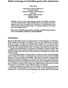
Figure 4. Double suspension surface. Each vertical straight line segment in ∂D is collapsed to a point, the bottom side of the square is identified with the top one Proof. For any open neighborhood U of Ψ one can find a system of partial isometries Ψ′ = {ψi′ : [a′i , b′i ] → [c′i , d′i ] ; i = 1, . . . , k} in U such that (1) the shifts c′i − a′i are pairwise commensurable; (2) no integral linear relation for the parameters of Ψ′ holds that is not a consequence of this commensurability and the balancedness of Ψ′ . Then the 1-form ω = dx on the handlebody HΨ′ ,y has pairwise commensurable periods over all integral cycles. Therefore, it is proportional to the pullback of the angular form dϕ on the circle S 1 under a map θ : HΨ′ ,y → S 1 . The connected components of the sets θ−1 (x), x ∈ S 1 , are the leaves of the foliation FΨ′ ,y induced by ω on HΨ′ ,y . The absence of additional relations on the parameters implies that any subset θ−1 (x) contains only one singularity of FΨ′ ,y . Therefore, the Euler characteristics χ(θ−1 (x)), which is a piecewise constant function of x, can jump only by one when x varies continuously. On the other hand, the balancedness of Ψ′ implies that χ(θ−1 (x)) averages to zero on S 1 . Therefore, for some x ∈ S 1 , we must have χ(θ−1 (x)) > 0, which means that at least one of the connected components of θ−1 (x) is a disc. The boundary ρ of this disc is a realization of some restriction r that holds for TΨ,y since ρ is homologous to zero in HΨ,y . For any Ψ′′ close enough to Ψ′ the restriction r will be realized also by TΨ′′ ,y . Now we consider a particular family of systems of partial isometries with k = 3 in which the subset of systems giving rise to minimal interval exchange transformations is precisely known, and explain the origin of Example 4. Let Ψ be an orientation preserving system of partial isometries of the form {ψi : [0, bi ] → [ci , 1], i = 1, 2, 3},

b 1 < b 2 < b 3 < c2 ,

c3 < b 3 ,

2b3 < b2 + c1 ,

bi + ci = 1,

and y ∈ (0, 1)6 be an arbitrary vector with y1 < y2 < . . . < y6 . The domain D and identifications in it b Ψ,y are shown in Fig. 4. to obtain Σ One can see from the left picture that the interval exchange transformation TΨ,y fills the double suspension surface and is associated with the following permutation: 1 2 3 4 5 6 7 π= 3 5 7 2 6 1 4

20


and the following vector of parameters:‘ a = (b1 , b2 + c1 − 2b3 , b3 − c3 , b3 − b2 , c2 − b3 , b2 − b1 , b1 ). The dashed lines in the left picture of Fig. 4 show the segments of separatrices between the singularity and the first intersection with [0, 1] × {0}. The corresponding foliation on the double suspension surface has two singularities each of which is a double saddle. If the excess e(Ψ) = b1 + b2 + b3 − 1 is not equal to zero, then TΨ,y is not minimal. In the case e(Ψ) = 0 the double suspension surface can be identified with the quotient of the regular skew polyhedron {4, 6 | 4} by Z3 , embedded in the 3-torus with the foliation induced by the 1-form (b2 + b3 ) dx1 + (b3 + b1 ) dx2 + (b1 + b2 ) dx3 , see [12, 15]. The minimality of TΨ,y is equivalent to Ψ being of thin type. This occurs if and only if the point (b1 : b2 : b3 ) ∈ RP 2 belongs to the Rauzy gasket, which is defined as follows. Denote by ∆ the following subset of the projective plane RP 2 : ∆ = {(x1 : x2 : x3 ) ; xi > 0, i = 1, 2, 3}, and by P1 , P2 , P3 , the projective transformations with matrices       1 1 1 1 0 0 1 0 0 0 1 0 , 1 1 1 , 0 1 0 , 0 0 1 0 0 1 1 1 1 respectively. Points of the Rauzy gasket are in one-to-one correspondence with infinite sequences (i1 , i2 , . . .) ∈ {1, 2, 3}N in which every element of {1, 2, 3} appears infinitely often. For any such sequence the intersection ∞ \ (Pi1 ◦ . . . ◦ Pim )(∆) m=1

consists of a single element, which is the point of the Rauzy gasket corresponding to the sequence. The interval exchange transformations from Example 4 was produced by using the construction above with the additional assumption b1 + b2 < b3 . One can see from the right picture in Fig 4 that the first return map for the shorter transversal [0, b2 + c3 ] will be the interval exchange transformation associated with the permutation 1 2 3 4 5 6 7 3 6 5 2 7 4 1 and the following vector of parameters: 1 (b1 , b2 + c1 − 2b3 , b3 − c3 , b3 − b1 − b2 , b1 , c2 − b3 , 2b2 − b3 ). b 2 + c3 The parameters ai , i = 1, 2, 3, and e from Example 4 are related to these as follows: a1 =

b1 , b 2 + c3

a2 =

b2 + c1 − 2b3 , b 2 + c3

a3 =

b 3 − c3 , b 2 + c3

e=

e(Ψ) b1 + b2 + b3 − 1 = . b 2 + c3 b 2 + c3

The triangle defined by ai > 0,

3a1 + 2a2 + 2a3 = 1

coincides with P3 (P2 (∆)), so it intersects the mentioned above Rauzy gasket in a subset that is also projective equivalent to the Rauzy gasket. 5.7. Interval translation mappings. Interval translation mappings were introduced by M. Boshernitzan and I. Kornfeld in [10]. Definition 17. An interval translation mapping is a map T : [0, 1) → [0, 1) of the form T (x) = x + ti

if

i−1 X j=1

λj 6 x