{solon.pissis, alexandros.stamatakis}@h-its.org. AbstractâIn this report, we focus on the efficient parallelisation of approximate string-matching algo- rithms ...
Minimising processor communication in parallel approximate string matching Christos Hadjinikolis and Costas S. Iliopoulos Department of Informatics King’s College London London, UK {christos.hadjinikolis, c.iliopoulos}@kcl.ac.uk
Abstract—In this report, we focus on the efficient parallelisation of approximate string-matching algorithms, which are based on dynamic programming, using the message-passing programming paradigm. We first present the decomposition and the mapping technique of the proposed parallel system. Then, we show a number of properties that follow from the application of this system, and use them to minimise the amount of point-to-point communication in each parallel step. We therefore provide a new cost-optimal parallel system, which can be directly and effectively applied to any approximate stringmatching algorithm with analogous characteristics. We show that, from a practical point of view, the proposed system reduces the time for pointto-point communication up to five times compared to the na¨ıve version of it, and that it can match, and also outperform, the classic parallel system introduced by Edmiston et al. in 1988. Finally, we provide a performance predictor that can be used to accurately and efficiently predict the performance of Edmiston’s and our system for given input data. Keywords-algorithms on strings; parallel algorithms; message-passing programming paradigm; dynamic programming; wave-front parallelism
I NTRODUCTION The problem of finding factors of a text similar to a given pattern has been intensively studied over the past decades, and it is a central problem for a wide range of applications, including signal processing [8], information retrieval [12], searching for similarities among biological sequences [11], file comparison [3], and spelling correction [9]. Approximate string matching, in general, consists in locating all occurrences of factors inside a text t that are similar to a pattern x. It consists in producing the positions of the factors of t that are at a distance of at most k from x, for a given natural number k. In particular, we consider the edit distance for measuring the approximation. The edit distance between two strings, not necessarily of the same length, is the minimum cost of
Solon P. Pissis and Alexandros Stamatakis Scientific Computing group Heidelberg Institute for Theoretical Studies Heidelberg, Germany {solon.pissis, alexandros.stamatakis}@h-its.org
a series of elementary edit operations to transform one string into the other. A parallel system is the combination of an algorithm and the parallel architecture on which it is implemented and executed. There has been ample work in the literature for devising parallel systems, using different models of computation, parallel architectures, and programming paradigms, for the approximate string-matching problem (cf. [1], [4], [7], [10]). Here, we focus on the efficient parallelisation of approximate string-matching algorithms, which are based on dynamic programming, using the message-passing programming (MPP) paradigm. As an example of an approximate stringmatching algorithm, one may consider any algorithm using the edit distance, such as the classic algorithm for computing the edit distance [8], algorithm M AX S HIFT [5] for fixed-length approximate string matching, the well-established algorithm for solving the longest common subsequence problem [12], or the Smith-Waterman algorithm [13] for performing local sequence alignment. The common characteristic of these algorithms is the computation of a dynamic-programming matrix D[0 . . n, 0 . . m], where n is the length of the text, and m ≤ n is the length of the pattern. Another key property is that each cell D[i, j] of the matrix can be computed only using cells D[i − 1, j], D[i − 1, j − 1], and D[i, j − 1]. We first present the decomposition and the mapping technique of the cost-optimal parallel system, introduced in [6], which makes use of wavefront parallelism in the MPP paradigm. Then, we demonstrate a number of properties that follow from the application of this system, and use them to minimise the amount of point-to-point communication in each parallel step. We therefore provide a new cost-optimal parallel system that can be directly and effectively applied to any approximate
string-matching algorithm with analogous characteristics. The rest of this report is structured as follows. In Section I, we describe the model of communication in the parallel computer. In Section II, we provide a detailed description of the proposed parallel system. In Section III, we present extensive experimental results, which demonstrate that the proposed system reduces the time for point-topoint communication up to five times compared to the one introduced in [6], and that it can match, and also outperform, the classic parallel system introduced by Edmiston et al. [1] in 1988. We also provide a performance predictor that can be used to accurately and efficiently predict the performance of these systems for given input data. We conclude in Section IV. I. M ODEL OF COMMUNICATION We make the following assumptions for the model of communication: (i) the parallel computer comprises a number of nodes and (ii) each node comprises one or several identical processors interconnected by a switched communication network. Although the latencies for intra- and inter-node communication can vary substantially in practice, we assume, as an abstraction, that the time taken to send a message of size s between any two nodes is independent of the distance between nodes, and can be modeled as tcomm = ts + stw , where ts is the latency of the message, and tw is the transfer time per data. The communication links between two nodes are bidirectional and singleported, that is, a message can be simultaneously transferred in both directions via the link, and only one message can be sent, and one message can be received at the same time. We assume that the input of size n + m is stored locally on each node. This can be achieved by using an initial, one-time-only, broadcast operation one-to-all in communication time (ts +(n+m)tw ) log p, which is asymptotically O(n log p), where p is the total number of available processors. II. T HE PROPOSED PARALLEL SYSTEM A. Decomposition technique We make use of the functional decomposition technique, in which the initial focus is on the computation that is to be performed, rather than on the data manipulated by the computation. The main observation for introducing parallelism is that cell D[i, j] can be computed using cells D[i − 1, j], D[i − 1, j − 1], and D[i, j − 1]. Based on this, if we partition the problem of computing
matrix D into a set {∆0 , ∆1 , . . . , ∆n+m } of antidiagonal arrays—also known as a sequence of parallel wavefronts of a computation—as shown in Equation 1, the computation of each cell in each diagonal is independent from the other cells of the same diagonal, and can be executed concurrently. The size of ∆ν , that is, the number of cells of ∆ν , is denoted by δν . D[ν − x, x] : 0 ≤ x ≤ ν D[ν − x, x] : 0 ≤ x < m + 1 ∆ν [x] = D[n − x, ν − n + x] : 0≤x r are neighbouring if and only if lνr = ∆ν [x] and fνq = ∆ν [x + 1], for some x, where 0 ≤ x < δν − 1. lνr
C. Properties of the system For each sequence ν − 2, ν − 1, ν of parallel steps, where 2 ≤ ν < n + m + 1, we distinguish among the following cases:
0
1
2
3
4
5
6
7
8
9
10
11
12
13
14
15
16
17
l3 13
0 1 3 f13
2 l2 13
3
·
4
·
2 f13
5
ց
l1 13
6
·
7
·
8
l2 23
ց
l0 13
10
· ·
1 f13
9
·
11
·
12 13
l3 23
0 f13
r=3
l1 23
1 f23 l0 23
16
·
17
0 f23
Figure 1.
r=2
2 f23
·
·
15
r=1
· ց
14
3 f23
r=0
Mapping of the cells of matrix D to the available processors for n = m = 17 and p = 4
1) δν−1 − δν−2 = 1 and δν − δν−1 = 1 2) δν−1 − δν−2 = 1 and δν − δν−1 = 0 3) δν−1 − δν−2 = 1 and δν − δν−1 = −1 4) δν−1 − δν−2 = 0 and δν − δν−1 = −1 5) δν−1 − δν−2 = 0 and δν − δν−1 = 0 6) δν−1 − δν−2 = −1 and δν − δν−1 = −1 For each set {D[i, j], D[i − 1, j], D[i, j − 1]} of cells, where 1 ≤ i ≤ n and 1 ≤ j ≤ m, we list the following immediate observations obtained from the problem decomposition (see Equation 1 in the Appendix): Observation 1: If δν − δν−1 = 0 and D[i, j] = ∆ν [x], then D[i−1, j] = ∆ν−1 [x] and D[i, j−1] = ∆ν−1 [x − 1], for some x, where 1 ≤ x < δν . Observation 2: If δν −δν−1 = −1 and D[i, j] = ∆ν [x], then D[i−1, j] = ∆ν−1 [x+1] and D[i, j − 1] = ∆ν−1 [x], for some x, where 0 ≤ x < δν − 1. Observation 3: If δν − δν−1 = 1 and D[i, j] = ∆ν [x], then D[i−1, j] = ∆ν−1 [x] and D[i, j−1] = ∆ν−1 [x − 1], for some x, where 1 ≤ x < δν . Lemma 1: If a processor r is assigned cell D[i, j] of ∆ν , such that ν > r, then r will also be assigned at least one of the cells D[i − 1, j] and D[i, j − 1] of ∆ν−1 . Proof: Without loss of generality, assume that cell D[i, j] = ∆ν [x] is mapped to processor r. Then, fνr ≤ x ≤ lνr holds. We distinguish among the following cases: 1) δν − δν−1 = 0: then, trivially, it holds r r fν−1 = fνr ≤ x ≤ lνr = lν−1 . From
Observation 1, D[i − 1, j] = ∆ν−1 [x], and, hence, D[i − 1, j] is mapped to r. 2) δν − δν−1 = −1: then, from Observation 2, D[i − 1, j] = ∆ν−1 [x + 1] and D[i, j − 1] = ∆ν−1 [x]. If the one extra cell of ∆ν−1 (δν − δν−1 = −1) is mapped to a r processor q > r, then it holds fν−1 = fνr r r r and lν−1 = lν . It follows that fν−1 = fνr ≤ r = lνr , hence, ∆ν−1 [x] is also x ≤ lν−1 mapped to r. If the one extra cell of ∆ν−1 is mapped to a processor q = r, then it holds r r = lνr + 1. It follows = fνr and lν−1 fν−1 r r r , that fν−1 = fν ≤ x + 1 ≤ lνr + 1 = lν−1 hence, ∆ν−1 [x+1] is mapped to r. If the one extra cell of ∆ν−1 is mapped to a processor r q < r, then it holds fν−1 = fνr + 1 and r r r lν−1 = lν + 1. It follows that fν−1 = r r r fν + 1 ≤ x + 1 ≤ lν + 1 = lν−1 , hence, ∆ν−1 [x + 1] is mapped to r. 3) δν − δν−1 = 1: then, from Observation 3, D[i − 1, j] = ∆ν−1 [x] and D[i, j − 1] = ∆ν−1 [x − 1]. If the one extra cell of ∆ν (δν − δν−1 = 1) is mapped to a processor r q > r, then it holds fν−1 = fνr and r r lν−1 = lνr . It follows that fν−1 = fνr ≤ x ≤ r = lνr , hence, ∆ν−1 [x] is also mapped lν−1 to r. If the one extra cell of ∆ν is mapped to r a processor q = r, then it holds fν−1 = fνr r r r r and lν−1 = lν −1. In case fν < x = lν , then r r , it holds fν−1 = fνr ≤ x−1 = lνr −1 = lν−1
hence, ∆ν−1 [x − 1] is mapped to r. In case r = fνr ≤ fνr ≤ x < lνr , then it holds fν−1 r r x ≤ lν − 1 = lν−1 , hence, ∆ν−1 [x] is mapped to r. If the one extra cell of ∆ν is mapped to a processor q < r, then it holds r r fν−1 = fνr − 1 and lν−1 = lνr − 1. It follows r r r that fν−1 = fν −1 ≤ x−1 ≤ lνr −1 = lν−1 , hence, ∆ν−1 [x − 1] is mapped to r. Lemma 2: There exist no four cells D[i, j], D[i − 1, j], D[i, j − 1], D[i − 1, j − 1], where 1 ≤ i ≤ n and 1 ≤ j ≤ m, the calculation of the content of which is mapped to more than two discrete neighbouring processors. Proof: Without loss of generality, assume that cell D[i, j] = ∆ν [x] is mapped to processor r. Then it holds fνr ≤ x ≤ lνr . We distinguish among the following cases: 1) δν−1 − δν−2 = 1 and δν − δν−1 = 1: From Observation 3, D[i − 1, j] = ∆ν−1 [x], D[i, j − 1] = ∆ν−1 [x − 1], and D[i − 1, j − 1] = ∆ν−2 [x − 1]. (a) If the one extra cell of ∆ν (δν − δν−1 = 1) is mapped to a processor q > r, then ∆ν−1 [x] is also mapped to r (see Lemma 1 Case 3). It follows that ∆ν−1 [x − 1] is allocated either to r or to r − 1. If ∆ν−1 [x − 1] is mapped to r then it r r holds fν−1 ≤ x − 1 < lν−1 . If the one extra cell of ∆ν−1 (δν−1 − δν−2 = 1) is mapped to a processor q > r then it holds r r r r . It follows = lν−1 and lν−2 = fν−1 fν−2 r r r r = lν−2 , that fν−2 = fν−1 ≤ x − 1 < lν−1 hence, ∆ν−2 [x − 1] is also mapped to r. If the one extra cell of ∆ν−1 (δν−1 −δν−2 = 1) is mapped to a processor q ≤ r then it holds r r r r fν−2 ≤ fν−1 and lν−2 = lν−1 −1. It follows r r r −1 = that fν−2 ≤ fν−1 ≤ x − 1 < lν−1 r lν−2 , hence, ∆ν−2 [x − 1] is also mapped to r. If ∆ν−1 [x − 1] is mapped to r − 1 then it r−1 r−1 holds fν−1 ≤ x − 1 = lν−1 . If the one extra cell of ∆ν−1 (δν−1 − δν−2 = 1) is mapped to a processor q > r−1 then it holds r−1 r−1 r−1 r−1 fν−2 = fν−1 and lν−2 = lν−1 . It follows r−1 r−1 r−1 r−1 , = lν−1 that fν−2 = fν−1 ≤ x − 1 = lν−2 hence, ∆ν−2 [x−1] is also mapped to r−1. If the one extra cell of ∆ν−1 (δν−1 −δν−2 = 1) is mapped to a processor q ≤ r − 1 then it r−1 r r . It follows that fν−2 = holds fν−2 = lν−1 x − 1, hence, ∆ν−2 [x − 1] is mapped to r.
(b) If the one extra cell of ∆ν (δν − δν−1 = 1) is mapped to a processor q ≤ r, then, we also have to examine the case when ∆ν−1 [x − 1] is also mapped to r, such that r r fν−1 ≤ x−1 = lν−1 (see Lemma 1 Case 3). It follows that ∆ν−1 [x] is mapped to r + 1. Similarly, as in the case when ∆ν−1 [x] is mapped to r, and ∆ν−1 [x − 1] is mapped either to r or to r − 1 (see Case 1(a)), we obtain that ∆ν−2 [x − 1] is mapped either to r or to r + 1. 2) δν−1 − δν−2 = 1 and δν − δν−1 = 0: From Observations 1 and 3, D[i−1, j] = ∆ν−1 [x], D[i, j − 1] = ∆ν−1 [x − 1], and D[i − 1, j − 1] = ∆ν−2 [x − 1]. Since δν = δν−1 , ∆ν−1 [x] is also mapped to r (see Lemma 1 Case 1). It follows that ∆ν−1 [x − 1] is mapped either to r or to r − 1. If ∆ν−1 [x − 1] is mapped to r then ∆ν−2 [x − 1] is also mapped to r (see Case 1(a)). If ∆ν−1 [x − 1] is mapped to r − 1, then ∆ν−2 [x − 1] is mapped either to r or to r − 1 (see Case 1(a)). 3) δν−1 − δν−2 = 1 and δν − δν−1 = −1: From Observation 2 and 3, D[i − 1, j] = ∆ν−1 [x + 1], D[i, j + 1] = ∆ν−1 [x], and D[i − 1, j − 1] = ∆ν−2 [x]. (a) If the one extra cell of ∆ν−1 (δν − δν−1 = −1) is mapped to a processor q > r, then ∆ν−1 [x] is also mapped to r (see Lemma 4 Case 2). It follows that ∆ν−1 [x + 1] is mapped either to r or to r + 1. ∆ν−2 [x] is mapped to r since ∆ν [x] is mapped to r and δν = δν−2 . (b) If the one extra cell of ∆ν−1 (δν − δν−1 = −1) is mapped to a processor q ≤ r, then ∆ν−1 [x + 1] is also mapped to r (see Lemma 4 Case 2). It follows that ∆ν−1 [x] is mapped either to r or to r − 1. ∆ν−2 [x] is mapped to r since ∆ν [x] is mapped to r and δν = δν−2 . 4) δν−1 − δν−2 = 0 and δν − δν−1 = −1: From Observation 1 and 2, D[i − 1, j] = ∆ν−1 [x + 1], D[i, j + 1] = ∆ν−1 [x], and D[i − 1, j − 1] = ∆ν−2 [x]. (a) If the one extra cell of ∆ν−1 (δν − δν−1 = −1) is mapped to a processor
q > r, then ∆ν−1 [x] is also mapped to r (see Lemma 4 Case 2). It follows that ∆ν−1 [x+1] is mapped either to r or to r+1. ∆ν−2 [x] is mapped to r since ∆ν−1 [x] is mapped to r and δν−2 = δν−1 . (b) If the one extra cell of ∆ν−1 (δν − δν−1 = −1) is mapped to a processor q ≤ r, then ∆ν−1 [x + 1] is also mapped to r (see Lemma 4 Case 2). It follows that ∆ν−1 [x] is mapped either to r or to r − 1. If ∆ν−1 [x] is mapped to r, then ∆ν−2 [x] is also mapped to r since δν−1 = δν−2 . If ∆ν−1 [x] is mapped to r − 1, then ∆ν−2 [x] is also mapped to r − 1 since δν−1 = δν−2 . 5) δν−1 − δν−2 = 0 and δν − δν−1 = 0: From Observation 1, D[i − 1, j] = ∆ν−1 [x], D[i, j + 1] = ∆ν−1 [x − 1], and D[i − 1, j + 1] = ∆ν−2 [x − 1].
the one extra cell of ∆ν−2 (δν−1 − δν−2 = −1) is mapped to a processor q < r then it r r r r holds fν−2 = fν−1 +1 and lν−2 = lν−1 +1. r r It follows that fν−2 = fν−1 + 1 < x + 1 ≤ r , hence, ∆ν−2 [x + 1] is also lνr + 1 = lν−2 mapped to r. If ∆ν−1 [x + 1] is mapped to r + 1 then it r+1 r+1 . If the one = x + 1 ≤ lν−1 holds fν−1 extra cell of ∆ν−2 (δν−1 − δν−2 = −1) is mapped to a processor q ≥ r+1 then it holds r+1 r+1 r+1 r+1 . It follows ≥ lν−1 and lν−2 = fν−1 fν−2 r+1 r+1 r+1 r+1 that fν−2 = fν−1 = x + 1 ≤ lν−1 ≤ lν−2 , hence, ∆ν−2 [x+1] is also mapped to r+1. If the one extra cell of ∆ν−2 (δν−1 − δν−2 = −1) is mapped to a processor q < r + 1 r+1 r . It follows that = fν−1 then it holds lν−2 r lν−2 = x+1, hence, ∆ν−2 [x+1] is mapped to r.
Since δν−1 = δν , ∆ν−1 [x] is also mapped to r (see Lemma 1 Case 1). It follows that ∆ν−1 [x − 1] is mapped either to r or to r − 1. If ∆ν−1 [x − 1] is mapped to r, then ∆ν−2 [x − 1] is also mapped to r since δν−2 = δν−1 . If ∆ν−1 [x − 1] is mapped to r − 1, then ∆ν−2 [x − 1] is also mapped to r − 1 since δν−2 = δν−1 .
(b) If the one extra cell of ∆ν−1 (δν − δν−1 = −1) is mapped to a processor q ≤ r, then ∆ν−1 [x + 1] is also mapped to r (see Lemma 4 Case 2). It follows that ∆ν−1 [x] is mapped either to r or to r − 1. Similarly as in the case when ∆ν−1 [x] is mapped to r, and ∆ν−1 [x + 1] is mapped either to r or to r + 1 (see Case 6(a)), we obtain that ∆ν−2 [x+1] is mapped either to r or to r−1.
6) δν−1 − δν−2 = −1 and δν − δν−1 = −1: From Observation 2, D[i−1, j] = ∆ν−1 [x+ 1], D[i, j + 1] = ∆ν−1 [x], and D[i − 1, j − 1] = ∆ν−2 [x + 1].
Lemma 3: For the computation of ∆ν , each processor only needs to send the content of a number of cells of ∆ν−1 to neighbouring processors.
(a) If the one extra cell of ∆ν−1 (δν − δν−1 = −1) is mapped to a processor q > r, then ∆ν−1 [x] is also mapped to r (see Lemma 4 Case 2). It follows that ∆ν−1 [x + 1] is allocated either to r or to r + 1. If ∆ν−1 [x + 1] is mapped to r then it holds r r fν−1 < x+1 ≤ lν−1 . If the one extra cell of ∆ν−2 (δν−1 − δν−2 = −1) is mapped to a r r = fν−1 processor q > r then it holds fν−2 r r r and lν−2 = lν−1 . It follows that fν−2 = r r r fν−1 < x + 1 ≤ lν−1 = lν−2 , hence, ∆ν−2 [x + 1] is also mapped to r. If the one extra cell of ∆ν−2 (δν−1 − δν−2 = −1) is mapped to a processor q = r then it holds r r r r +1. It follows = lν−1 and lν−2 = fν−1 fν−2 r r r that fν−2 = fν−1 < x + 1 ≤ lν−2 = lνr + 1, hence, ∆ν−2 [x + 1] is also mapped to r. If
Proof: Let us assume that for the computation of cell D[i, j] = ∆ν [x] mapped to a processor r, processor r − 1 (resp. r + 1 by Lemma 2) needs to send the content of cell D[i − 1, j − 1] of ∆ν−2 to r. This implies that, for the calculation of ∆ν−1 , it was not necessary for processor r − 1 (resp. r + 1) to send the calculated content of D[i−1, j−1] to r. This further implies that neither cell D[i, j −1] nor D[i−1, j] of ∆ν−1 were mapped to r. Hence, since cell D[i − 1, j − 1] of ∆ν−2 was mapped to r − 1 (resp. r+1), then both of these cells must also have been mapped to r − 1 (resp. r + 1) by Lemma 2. But if those cells were mapped to r−1 (resp. r+1) for calculating ∆ν−1 , it is definitely the case that cell D[i, j] of ∆ν will also be mapped to r − 1 by Lemma 1. Thus, we obtain a contradiction, and the lemma holds. Corollary 1: For the computation of ∆ν , each processor only needs to receive the content of
a number of cells of ∆ν−1 from neighbouring processors. Proof: Direct consequence of Lemma 3. Lemma 4: For the computation of ∆ν , processor r needs to receive the contents of at most two r−1 r+1 cells, ∆ν−1 [lν−1 ] and ∆ν−1 [fν−1 ], from neighbouring processors r − 1 and r + 1, respectively. Proof: Without loss of generality, assume that cell D[i, j] is mapped to processor r. From the proof of Lemma 2, we distinguish among the following cases (see Fig. 2 in this regard): 1) D[i − 1, j], D[i, j − 1], and D[i − 1, j − 1] are mapped to r. 2) D[i − 1, j] is mapped to r, and D[i, j − 1] and D[i − 1, j − 1] are mapped to r − 1. 3) D[i − 1, j] and D[i − 1, j − 1] are mapped to r, and D[i, j − 1] is mapped to r − 1. 4) D[i, j − 1] is mapped to r, and D[i − 1, j] and D[i − 1, j − 1] are mapped to r + 1. 5) D[i, j − 1] and D[i − 1, j − 1] are mapped to r, and D[i − 1, j] is mapped to r + 1. We eliminate Case 1 since all cells are mapped to r. By Lemma 3 and Corollary 1, the problem is reduced to the following two cases: • D[i − 1, j] is mapped to r and D[i, j − 1] is mapped to r − 1. Clearly, r − 1 needs to r−1 ] to r for the send D[i, j − 1] = ∆ν−1 [lν−1 computation of D[i, j]. • D[i, j − 1] is mapped to r and D[i − 1, j] is mapped to r + 1. Clearly, r + 1 needs to r+1 send D[i − 1, j] = ∆ν−1 [fν−1 ] to r for the computation of D[i, j].
r−1
r
r+1
Figure 2. The five possible mappings of the set of cells {D[i, j], D[i − 1, j], D[i, j − 1], D[i − 1, j − 1]} to processors r − 1, r, and r + 1, given that D[i, j] is mapped to r
Corollary 2: For the computation of ∆ν , processor r needs to send the contents of at most two r−1 r+1 cells, ∆ν−1 [lν−1 ] and ∆ν−1 [fν−1 ], to neighbouring processors r − 1 and r + 1, respectively. Proof: Direct consequence of Lemma 4. D. Processor communication Algorithm PP-C OMM provides the point-topoint communication between r, r − 1, and r + 1
at step ν. It takes as input the size n of the text, the diagonal array ∆ν , the indices fνr and lνr of the first and the last cell of ∆ν mapped to processor r, respectively. It also needs as input the indices r r fν+1 and lν+1 of the first and the last cell of ∆ν mapped to processor r, respectively. By Observations 1–3, we obtain two cases: the case where ν < n (Algorithm PP-C OMM line 1) by Observations 1 and 3 (δν − δν−1 ∈ {0, 1}), and the case where ν ≥ n (Algorithm PP-C OMM line 10) by Observation 2 (δν −δν−1 = −1). By Corollary 2, for the computation of ∆ν+1 , processor r needs to send the contents of at most two cells, ∆ν [fνr ] and ∆ν [lνr ], to neighbouring processors r − 1 (Algorithm PP-C OMM lines 5 and 14) and r + 1 (Algorithm PP-C OMM lines 3 and 12), respectively. Hence, the data exchange between the processors in Algorithm PP-C OMM involves a constant number of point-to-point message transfers at each step. Since the number of cells to be computed is Θ(nm), the number of parallel steps is Θ(n)—exactly n + m + 1 diagonals—and each processor is assigned the computation of O(m/p) cells—the size of each diagonal is O(m)—at each parallel step, we obtain the following result. Theorem 1: The proposed parallel system is cost-optimal. ALGORITHM PP-C OMM(r, n, ν, ∆ν , fνr , lνr , r r ) , lν+1 fν+1 1: if ν < n then r r 2: if (fν+1 ≤ lνr + 1 ≤ lν+1 ) = false then r 3: r sends ∆ν [lν ] to r + 1 r r ) = false then 4: if (fν+1 ≤ fνr ≤ lν+1 r 5: r sends ∆ν [fν ] to r − 1 r − 1 ≤ lνr ) = false then 6: if (fνr ≤ fν+1 7: r receives ∆ν [fνr ] from r − 1 r ≤ lνr ) = false then 8: if (fνr ≤ lν+1 9: r receives ∆ν [lνr ] from r + 1 10: else r r ) = false then ≤ lνr ≤ lν+1 11: if (fν+1 r 12: r sends ∆ν [lν ] to r + 1 r r 13: if (fν+1 ≤ fνr − 1 ≤ lν+1 ) = false then r 14: r sends ∆ν [fν ] to r − 1 r + 1 ≤ lνr ) = false then 15: if (fνr ≤ lν+1 16: r receives ∆ν [lνr ] from r + 1 r ≤ lνr ) = false then 17: if (fνr ≤ fν+1 18: r receives ∆ν [fνr ] from r − 1 Furthermore, if D[i − 1, j] = ∆ν [lνr ] is the last cell mapped to r in step ν, then, by checking if D[i, j] is mapped to r (Algorithm PP-C OMM lines 2 and 11), we know whether r should send the
10000
1000
Elapsed time [log s]
content of D[i − 1, j] to r + 1 or not. Analogously, if D[i, j −1] = ∆ν [fνr ] is the first cell mapped to r in step ν, then, by checking if D[i, j] is mapped to r (Algorithm PP-C OMM lines 4 and 13), we know whether r should send the content of D[i, j − 1] to r − 1 or not. Hence we obtain the following result: Theorem 2: The point-to-point communication in Algorithm PP-C OMM is minimal for the proposed parallel system.
p=1 p=12 p=24 p=48 p=96 p=192 p=384
100
10
1 100000
200000
400000
500000
(a) Elapsed time of OPASM 400
350
300
250 Speed-up [-]
In order to evaluate the parallel efficiency of the proposed parallel system, we implemented algorithm M AX S HIFT in the C programming language, and parallelised it using the Message Passing Interface (MPI), which supports the MPP paradigm, implementing programme OPASM, which uses the proposed optimised parallel system. DNA sequences of the single chromosome of Escherichia coli str. K-12 substr. MG1655, obtained from GenBank [2], were used as input for the programme. Experimental results regarding the elapsed time of OPASM for different problem sizes are provided in Fig. 3a. The measured relative speed-up of OPASM is illustrated in Fig. 3b. The relative speed-up was calculated as the ratio of the runtime of the parallel algorithm on 1 processor to the runtime of the parallel algorithm on p processors—the runtime of the parallel algorithm on 1 processor was identical to the sequential one. The experiments highlight the good scalability of OPASM, even for small problem sizes. When increasing the problem size, OPASM achieves linear speed-ups and confirms our theoretical results. In order to relate the amount of point-to-point communication of OPASM to other parallel systems, we also parallelised algorithm M AX S HIFT with MPI, implementing programme PASM, which uses the parallel system introduced in [6]. The only difference from OPASM is that processor communication in PASM involves point-to-point boundary cell swaps between all neighbouring processors at each parallel step. Two different versions were used for each of the two programmes: one with blocking send operations (MPI Send); and one with blocking synchronous send operations (MPI Ssend). We measured the elapsed point-to-point communication time of PASM and OPASM (Algorithm PP-C OMM) for different problem sizes by commenting out the computation phase of both programmes. The main contribution of this report becomes apparent from Fig. 4: (i) the time for point-to-point communication of OPASM
300000 Text length [bp]
III. E XPERIMENTAL RESULTS
200
150
100
50 Linear speed-up Measured speed-up
0 1 12 24
48
96
192
384
Number of processors [-]
(b) Measured speed-up of OPASM Figure 3. Elapsed time of OPASM for n = m, and measured speed-up of OPASM for n = m = 500K
is reduced up to five times with blocking send operations (Fig. 4a) and up to ten times with blocking synchronous send operations (Fig. 4b); (ii) at a certain point, the amount of point-to-point communication of OPASM becomes essentially constant (note that, the curves of OPASM on 96 and 192 processors coincide both, in Fig. 4a and in Fig. 4b). In order to relate the overall performance of OPASM to other parallel systems, we parallelised algorithm M AX S HIFT with MPI, implementing programme EDM, which uses the classic parallel system introduced by Edmiston et al. Since latency of communication ts is usually much worse than communication bandwidth tw , the system by Edmiston et al. strives to minimise the number of point-to-point communications by sending the content of Θ(m/p) cells Θ(p) times—while the proposed parallel system sends the content of O(1) cells Θ(n) times. In the system proposed by Edmiston et al., the dynamic-programming matrix is decomposed into a p × p matrix of submatrices. Each processor q, 0 ≤ q < p, is assigned a row of p submatrices, and processor q, q > 0, starts computing the first submatrix of its row
100
PASM p=48 OPASM p=48 PASM p=96 OPASM p=96 PASM p=192 OPASM p=192
EDM 768K x 768K OPASM 768K x 768K EDM 384K x 384K OPASM 384K x 384K
700
600
Elapsed time [s]
Elapsed time [log s]
500
10
400
300
200
100
1 1e+06
0 2e+06
3e+06
4e+06
48
96
Text length [bp]
192
384
Processors [-]
(a) Blocking send 100000
PASM p=48 OPASM p=48 PASM p=96 OPASM p=96 PASM p=192 OPASM p=192
Figure 5. Elapsed time of EDM and OPASM for n = m = 384K and n = m = 768K
1000
100 1e+06
2e+06
3e+06
4e+06
Text length [bp]
(b) Blocking synchronous send Figure 4. Elapsed time of the point-to-point communication of PASM and OPASM with blocking send operation and blocking synchronous send operation
only when processor q − 1 has already computed the first submatrix of its row, resulting in a total of 2p − 1 parallel steps. When q, q < p − 1, finishes the computation of a submatrix, it must send Θ(m/p) cells (the last row) of the submatrix that has been computed to processor q + 1. Hence, in total, this system communicates only Θ(p) times. This approach exhibits two disadvantages: (i) the matrix size in either dimension must be a multiple of the number of processors; (ii) since processor q does not start computing until step q, this generates load imbalance, in particular for large submatrices. We used the aforementioned dataset as input for EDM and OPASM. The elapsed times of EDM and OPASM are provided in Fig. 5. These experimental results confirm our theoretical findings: OPASM is more efficient than EDM for small processor counts and problems of large size. However, as we increase the number of processors, the size of submatrices computed by EDM decreases, and the two systems exhibit comparable performance. Finally, we also implemented programme PRE, a performance predictor for EDM and OPASM. PRE
uses the theoretical results presented in [1] and in Section II to accurately and efficiently predict the performance of EDM and OPASM, respectively. The performance of EDM can be predicted by measuring the sum of the processor idle time, the sum of per submatrix calculation time, and the sum of communication times for Θ(m/p) cells. The performance of OPASM can be predicted by measuring the sum of calculation time per antidiagonal, and the sum of communication costs times for exchanging O(1) (at most two) cells per anti-diagonal. Experimental results for the performance prediction of EDM and OPASM are provided in Fig. 6. The results demonstrate that the predictor is highly accurate. PRE only takes a few seconds to execute. It performs a number of iterations to measure the aforementioned average time costs. Users can chose to increase the number of iterations in the predictor to further increase its accuracy at the expense of longer predictor runtimes. 200
EDM PRE EDM OPASM PRE OPASM
150
Elapsed time [s]
Elapsed time [log s]
10000
100
50
0 48
96
192
Processors [-]
Figure 6.
Performance prediction for n = m = 384K
The experiments were conducted on an Infiniband-connected cluster using 1 up to 384 2.4 GHz AMD 6136 processors under the Linux operating system. The implementations of OPASM, EDM, and PRE are available at a website (http: //www.exelixis-lab.org/solon) under the terms of the GNU General Public License. IV. C ONCLUSION In this report, we presented a new costoptimal parallel system based on MPP paradigm for efficient parallelisation of approximate stringmatching algorithms. From a practical point of view, our experimental results show that the proposed system reduces the time for point-to-point communication up to five times compared to the one introduced in [6], and that it can match, and also outperform, the classic parallel system introduced by Edmiston et al. [1]. Finally, we designed and implemented a performance predictor that can be used to accurately and efficiently predict the performance of these systems given a specific input dataset. We also tested other dynamicprogramming kernels with the presented parallel systems obtaining similar results. Our immediate goal is to design, implement, and test a new hybrid system, between the one proposed here and the one proposed by Edmiston et al., that will make use of the proposed system only for the load imbalanced parallel steps of the system proposed by Edmiston et al. R EFERENCES [1] E. Edmiston, N. Core, J. Saltz, and R. Smith. Parallel processing of biological sequence comparison algorithms. International Journal of Parallel Programming, 17:259–275, 1988. [2] GenBank. http://www.ncbi.nlm.nih.gov/genbank/, June 2012. [3] P. Heckel. A technique for isolating differences between files. Communications of the ACM, 21(4):264–268, 1978. [4] X. Huang. A space-efficient parallel sequence comparison algorithm for a message-passing multiprocessor. International Journal of Parallel Programming, 18(3):223–239, 1990. [5] C. Iliopoulos, L. Mouchard, and Y. Pinzon. The Max-Shift algorithm for approximate string matching. In G. Brodal, D. Frigioni, and A. Marchetti-Spaccamela, editors, Proceedings of the fifth International Workshop on Algorithm Engineering (WAE 2001), volume 2141 of Lecture Notes in Computer Science, pages 13–25, Denmark, 2001. Springer.
[6] C. S. Iliopoulos, L. Mouchard, and S. P. Pissis. A parallel algorithm for the fixed-length approximate string matching problem for high throughput sequencing technologies. In B. Chapman, F. Desprez, G. R. Joubert, A. Lichnewsky, F. Peters, and T. Priol, editors, Proceedings of the International Conference on Parallel Computing (PARCO 2009), volume 19 of Advances in Parallel Computing, pages 150–157, France, 2010. IOS Press. [7] G. M. Landau and U. Vishkin. Fast parallel and serial approximate string matching. Journal of Algorithms, 10(2):157–169, 1989. [8] V. I. Levenshtein. Binary codes capable of correcting deletions, insertions, and reversals. Technical Report 8, Soviet Physics Doklady, 1966. [9] J. L. Peterson. Computer programs for detecting and correcting spelling errors. Communications of the ACM, 23(12):676–687, 1980. [10] S. Rajko and S. Aluru. Space and time optimal parallel sequence alignments. IEEE Transactions on Parallel and Distributed Systems, 15:1070– 1081, 2004. [11] P. H. Sellers. On the theory and computation of evolutionary distances. SIAM Journal on Applied Mathematics, 26(4):787–793, 1974. [12] R. A. Wagner and M. J. Fischer. The string-tostring correction problem. Journal of the ACM, 21(1):168–173, 1974. [13] M. S. Waterman and T. F. Smith. Identification of common molecular subsequences. Journal of Molecular Biology, 147(1):195–197, 1981.