Proc. of the 2013 8th International Conference on System of Systems Engineering, Maui, Hawaii, USA - June 2-6, 2013
Minimizing Energy Consumption in Random Walk Routing for Wireless Sensor Networks utilizing Compressed Sensing Minh Tuan Nguyen School of Electrical and Computer Engineering Oklahoma State University Stillwater, OK 74078 Email:
[email protected]
Abstract—Random walk (RW) routing for Wireless Sensor Networks (WSNs) has been proven to balance energy consumption for the whole sensors. Since Compressive sensing (CS) provides a novel idea that can reconstruct all raw data based on a small number of measurements, the energy consumption for data gathering in WSNs is reduced significantly. The combination between RW routing and CS can help efficiently save energy and achieve longer network lifetime. In this paper, we continue to introduce RW as an effective routing method in WSNs utilizing CS. We formulate the mean value of the communication distance between sensors in a RW and the mean distance between RWs and the base station (BS) statistically. We finally build the total energy consumption and exploit the minimum energy consumption case for the network. Based on analyzing the sensor broadcasting radius, while the WSN is connected as an undirected graph G(V, E), we can suggest the optimal radius that leads the network consumes the least energy and even has load balancing. Index Terms—Wireless sensor networks, compressive sensing, random walk, routing.
I. I NTRODUCTION The recent advancement of Wireless Sensor Networks (WSNs) in both military and civil applications motivates us to work on data gathering problems. Our goal is to prolong the sensor lifetime and keep the network connected as long as possible. We start with Compressed Sensing (CS) [1] applied to WSNs which helps significantly reduce the consumed energy while collecting data. Based on the correlation of the sensing data or sensor readings that makes them compressible, the network only needs to transmit a limited number of measurements related to the large significant coefficients of the whole data. All the raw data can be recovered precisely at the base station (BS). Since [2] states that random sparse measurement matrix can work as good as the Gaussian dense matrix in CS, Random Walk (RW) [3] fortunately combines with CS techniques to provide a very effective routing method for WSNs. In [4], a RW collects sensor readings through each random step. It keeps adding sensor readings from nodes which it walks through and finally sends the combination of measurements to the BS for CS recovery processes. In RW theory, the length of a RW is considered as the mixing time that depends on the neighborhood matrix or the
978-1-4673-5597-1/13/$31.00 ©2013 IEEE
transition matrix that will be addressed in the next section. The neighborhood matrix is a square matrix that expresses the connections between every node in the network by its entries zero or one. We know that sensors communicate by using the transmitting radius. So, the length of the radius decides the size of the sensor neighborhood. In other words, if we increase or decrease the broadcast radius, the network or the graph connection will be stronger or weaker. Based on that, in our paper, we formulate the total energy consumption for a WSN applied CS and RW routing as stated above. A minimum radius is chosen to ensure that all sensor are connected. The random connected network can be considered as a undirected graph G(V, E), where V is the vertex set and E is the edge set. As the radius is increased, each node connects to more nodes, or more edges from it will be set. This results in a stronger connection for the network or the graph. This will reduces the length of RWs. We exploit the trade-off between the transmitting radius and the RW length to derive the minimum energy consumption for the network. This paper is organized as follows: we briefly introduce CS, RW and related works in Section II. We are going to formulate of our problem in section III and show some simulation results in section IV. The rest of this paper contains the conclusions and future work. II. BACKGROUND AND R ELATED WORKS A. Brief introduction to CS Compressed Sensing techniques [1], [5], [6], [7] bring us a sound approach to recover a compressible signal from undersampled random projections, also refer to as measurements. A compressible vector signal x ∈ RN ( x = [x1 x2 . . . xN ]T ) is k-sparse if x has k non-zero elements. In another case, x may be dense (most elements of x are non-zeros) but can be considered as sparse in ψ domain if x = ψθ and θ is a k-sparse vector. When applying CS to a WSN, vector x represents data from N sensors in the network. The gain when we apply CS is that the number of measurements is much less than the number of the original sensing data. Vector y, called the measurement vector, contains data sampled from N sensor
297
readings; y ∈ RM ( y = [y1 y2 . . . yM ]T ), where M ≪ N [1][7]. Signal Sampling: The random measurements are generated by y = ϕx where ϕ ∈ RM ×N is often a full-Gaussian matrix or binary matrix, M called projection ∑N matrix. y ∈ R is the measurement vector with yi = j=1 φi,j xj , where φi,j are all entries on the ith row of our projection matrix ϕ. Signal Recovery: The number of measurement required to reconstruct the original signal perfectly with high probability is M = O (k log N/k) following the l1 optimization problem given by [7]. x ˆ = arg min || x ||1 , subject to y = ϕx.
C. Related works Random walk has been used effectively for data gathering in WSNs [9] [10] [11]. It does not need global information as the shortest path routing and furthermore, it achieves load balancing for the networks. It becomes more of a powerful routing method when combined with Compressive sensing [1] [5] since the sparse random projection has been proven that it can work as good as the dense the full Gaussian matrix in [2] [12]. [4] introduces RW routing for WSNs using CS based on the distributed compressed sensing (DCS) [13]. It also proves that RW works better than the shortest path routing in this case. 1
(1)
In case we need sparsifying matrix to have x sparse in ψ domain (ψ can be Wavelet or DCT depending on our signal properties)
r1
2
3 r2
4
5 BS
6
7
8
ˆθ = arg min || θ ||1 , subject to y = ϕψθ, (2) ∑n where || θ ||1 = i=1 |θi | . The l1 optimization problem can be solved with linear programming techniques such as Basis Pursuit (BP) [1]. In reality, we have to consider the noise while sampling and sending the measurements (in our case we collect measurements and send to the base-station) : y = ϕx + e , with || e ||2 < ϵ and recover x ˆ = arg min || x′ ||1 , subject to ||y = ϕx′ ||2 < ϵ.
(3) Fig. 1.
Illustration of a simple RW routing and the projection matrix
B. Random Walk Random walk (RW) on a graph can be modeled as a Markov Chain mentioned in [3] [8]. Walking steps jump from node to node randomly based on a probability defined by the graph. Specifically, the next node j in the sequence is selected from the set of neighbors of the previous node i in the sequence with probability Pij , also called transition probability. The probabilities form a transition matrix P = [Pij ]. For a simple random walk, if at time k, we are at vertex i, choose uniformly an adjacent vertex j to move to with probability Pij . Let d(i) denote the degree of vertex i, then { Pi,j = P (Xk+1 = j | Xk = i) =
1 d(i) ,
0,
if i, j ∈ E others
(4)
In a WSN with a large number of nodes, the graph is created with the connections between nodes and their neighbors. These communication links are based on the broadcasting radius of sensor nodes. In this way, the number of neighbors depends on the energy each node spends to broadcast its information. Definition: Mixing time is a number of steps before the distribution of a random walk be stationary. It shows how fast a RW converges to its stationary distribution. Since we need to sample all sensors equally, RWs have the mixing time approaches uniform stationary distribution that is calculated in the analysis section.
In Fig. 1, a RW samples at only two nodes. It adds two sensor reading S1 and S2 including two coefficients r1 and r2 that respectively multiply to S1 and S2 into the first measurement. It is illustrated in the measurement matrix at the 1st row corresponding to the 1st RW. Another node that is chosen randomly to initiate the second RW. In the second row of the measurement matrix, the entries show the coefficients that multiply corresponding to the nodes’ readings are sampled by the 2nd RW. M RWs will collect enough the number of measurements required to reconstruct precisely all raw data from the network at the BS. Based on the RW theory, we find out the trade-off between the length of a RW and the broadcasting radius of sensors. The idea is also mentioned in [14]. We will formulate the total energy consumption for WSNs using CS and RW. The optimal broadcasting radius is suggested for a WSN to achieve the lowest energy consumption. III. P ROBLEM FORMULATION A. Network model We model a WSN with N sensors which are uniformly randomly distributed to a square area L × L. The topology of the connected network is a random geometric graph G(V, E). We assume that each sensor has the same maximum broadcasting radius called R calculated by a Euclidean distance. In reality,
298
our network is not a regular network where each sensor has a different number of neighbors in its range of the radius R. If we change the value of R, the connection of the graph will change as follows: the set of vertex is the same based on the total number of sensors, but the edge set changes based on the communication between sensors in each neighborhood. We analyze this graph in the next section. B. Analysis Based on CS theory, we need a number of measurements required (M ) from the network to recover all raw sensor readings at the BS, so the network needs to generate M RWs to collect reading data. M nodes are chosen randomly with a probability as M N to initiate M data collection walks. In each RW, an initiated node adds its reading into the message and then forwards the combined data to one of its neighbors chosen by a probability called transition probability Pij . Sensor nodes that belong to the RWs receive the message and have the same process: adding their own data and forwarding messages to their neighbors. The sampling processes finish when the number of walking steps reaches the length of the RW, also called the mixing time of the graph G(V, E). The mixing time of RWs has been studied well in [8] [15] [16] showing that it significantly depends on the maximum radius or the transition probability Pij . As mentioned in [8], the asymptotic rate of convergence of the Markov chain to the uniform equilibrium distribution is determined by the second largest eigenvalue of the transition matrix P as follows: µ(P ) = maxi=2,...,n |λi (P )| = max[λ2 (P ), .λn (P )]
(5)
Since the graph is irreducible and aperiodic, then µ(P ) < 1 and the distribution converges to uniform asymptotically. The mixing time τ can be calculated as: τ = 1/log(1/µ)
(6)
sensors are uniformly distributed as shown in Fig. 2, we can calculate the mean communication distance statistically as follows: ∫ ∫ E[r2 ] = (x2 + y 2 ) ρ(x, y) dx dy (7) As we assume sensors are uniformly distributed in the area with the radius R, and ρ = 1/(πR2 ) is the joint probability (pdf) with two random variables x and y. r is also a random variable presenting the real distance between consecutive sensors along a RW (Fig. 2). We can change equation (7) into polar coordinates: ∫ ∫ E[r2 ] = r′2 ρ(r′ , θ) r′ dr′ dθ (8)
E[r2 ] =
1 πR2
∫
2π
θ=0
∫
R
r′3 dr′ dθ.
(9)
r=0
Finally, we obtain: R2 2
(10)
R rmean = √ 2
(11)
E[r2 ] = or
We can now formulate the total energy consumption Etotal of our network after M measurements required are sent to the BS Etotal = M (τ E[rα ] + E[dα ]) (12) where α ≥ 2 (it is shown in [17] that α = 2 and α = 4 in free space and multipath fading channels, respectively). d presents the transmitting distance between the last step of a RW and the BS that can be considered as a random variable. Since sensors and RWs are initiated uniformly randomly, we can calculate the mean value of d approximately in two common positions for the BS: BS at the center of the sensing area and BS outside the sensing area.
R
R
BS
Real communication distance (r)
Fig. 2.
Sensor neighborhood defined by the maximum broadcasting radius
In order to build a general formula for the total energy consumption Etotal , we need to calculate the distances of hops along each RW. Sensor nodes have the same maximum radius R in forming the neighborhoods but they spend different energy for transmitting data to different neighbors. Since
299
Sensor node
Fig. 3.
Flow of data
BS at the center of sensing area
LxL
1) BS at the center of the sensing area: In Fig. 3, a RW ends at a node that is also randomly distributed in the whole network. We can calculate the mean square distance as follows: ∫
L
∫
L
[(x −
E[d2 ] = 0
0
L 2 L ) + (y − )2 ]f (x, y)dxdy, (13) 2 2
where f (x, y) = L12 is the joint probability function (pdf). We can obtain the expected square distance from RWs to the BS: L2 . (14) 6 We finally derive the total energy consumption for WSNs from (12) as follows: E[d2 ] =
IV. S IMULATION R ESULTS We consider a WSN with N = 500 sensors uniformly randomly distributed in the square sensing area 100 × 100 (L = 100). We work with 90 RWs that provide the number of measurements required to recover precisely all raw sensor readings M = 90. We chose by chance dmean = 200 as the mean distance between RWs and the BS. The path-loss exponent for all communication distances is chosen as α = 2.5. As we assumed, every node has the same broadcasting radius R. We start with R = 10 to keep the network always connected. Since we keep increasing R, the number of sensors in each neighborhood in our graph increases as shown in Fig.5. The maximum number of sensors in each neighborhood is equal to the total number of sensors in the whole network.
R2 α/2 L2 ) + ( )α/2 ) (15) 2 6 We are going to analyze the other case for BS’s position.
Average number of neighbors versus maximum radius
Etotal = M (τ (
450 400 Average number of sensors
Sensor node
500
Flow of data
L
350 300 250 200 150 100 50
L /2
0
0.5
Fig. 5.
Fig. 4.
Li
BS outside the sensing area
2) BS outside the sensing area: As shown in Fig. 4, BS is located outside the sensing area. We set a fixed position for BS (Li , L2 ) in this analysis section. It means Li can be changed versus L in real applications. The expected square distance between RWs and BS: ∫
L
∫
1.5
The average number of neighbors when changing R
Based on the connected graph, we derive the probability transition matrix Pij that follows the equation (4). The number of steps required to converge to the the uniform distribution asymptotically reduce when the broadcasting radius of sensors R increases, as shown in Fig.6. The average mixing time and the broadcasting radius 120
100
Average mixing time
L
0
1 R/L
Base Station
L
L E[d2 ] = [(x − Li )2 + (y − )2 ]f (x, y)dxdy (16) 2 0 0 Similarly, we obtain the mean square distance between RWs and BS as follows:
80
60
40
20
L3 L2 1 (L − Li )3 + i]+ (17) E[d2 ] = [ L 3 3 12 From (12) and (17), we derive the formula for the total energy consumption when BS is outside the sensing area: R2 α/2 (L − Li )3 + L3i L2 α/2 ) +( + ) ] (18) 2 3L 12 We now have built all total energy consumption formulas. They will be all applied for a real network in the simulation section. Etotal = M [τ (
0 0.1
0.15
0.2
0.25
R/L
Fig. 6.
The mixing time reduces when the radius increases
As we receive the lengths of RWs corresponding with the transmitting radii as mentioned above, we can calculate the total energy consumption for our network. Fig. 7 shows the average energy consumption at each radius value. We can see that the network consumes the lowest energy at R = 14 or at
300
Compare two projection matrices: Full Gaussian and Sparse Binary
the rate R/L = 0.14. Based on these results, we can suggest the optimal radius for the sake of prolonging the network life. 7
x 10
0.21
The total energy consumption versus transmitting radius
0.2 Average Reconstruction Error
5.234
0.22
Total energy consumption
5.232
5.23
5.228
Sample all (full Gaussian) Sample by Random Walk
0.19 0.18 0.17 0.16 0.15
5.226
0.14 5.224
0.13 60 5.222
5.22 10
Fig. 8. 15 20 The length of the maximum radius
65
70 75 80 Number of measurements
85
90
CS reconstruction with the lowest energy consumed RW
25
Fig. 7. Total energy consumption of the network versus sensor broadcasting radius
The total energy consumption is minimized at R = 14 when the RW length is τ = 48 as showed in Fig. 6. Only 48 random nodes are walked through or sampled by one RW for building each measurement. It also means that the corresponding row in the projection matrix has only 48 nonzero elements. As mentioned in [2], an appropriate sparse binary projection matrix can work as good as a full-Gaussian matrix for k-sparse signals with different k values. We also have worked on real temperature sensor readings with different number of RWs from 60 to 90. Normalized reconstruction ||x−ˆ x|| errors ( ||x||2 2 ) taken from the CS reconstruction processes with the two different projection matrices are compared. It is shown in Fig. 8 that the optimum length RW works well for either energy saving and CS reconstruction. V. C ONCLUSIONS AND F UTURE WORK In this paper, we exploit the distance of the broadcasting radius of sensors in a WSN applied CS and RW routing to obtain the lowest energy consumption level. We have used simple RWs to collect data for WSNs, applied CS to recover all sensor readings based on the measurements received at the BS. We also enrich our results by providing the formulas of the mean distances in two common positions for the BS: BS at the center and BS outside the sensing area. We show by experiments and suggest the optimal transmitting radius for sensors based on the lowest total energy consumption. In future work, we will study to exploit the sparsity of the projection matrix to save the energy consumption for routing methods in WSNs utilizing CS. R EFERENCES [1] D.L.Donoho, “Compressed sensing,” Information Theory, IEEE Transactions on, vol. 52, pp. 1289 – 1306, 2006. [2] R. Berinde and P. Indyk, “Sparse recovery using sparse random matrices,” 2008. [3] L. Lovsz, “Random walks on graphs: A survey,” 1993.
[4] M. Sartipi and R. Fletcher, “Energy-efficient data acquisition in wireless sensor networks using compressed sensing,” in Data Compression Conference (DCC), 2011, pp. 223 –232, March 2011. [5] E. Candes, J. Romberg, and T. Tao, “Robust uncertainty principles: exact signal reconstruction from highly incomplete frequency information,” Information Theory, IEEE Transactions on, vol. 52, pp. 489 – 509, Feb. 2006. [6] N. Rahnavard, A. Talari, and B. Shahrasbi, “Non-uniform compressive sensing,” in Communication, Control, and Computing (Allerton), 2011 49th Annual Allerton Conference on, pp. 212 –219, Sept. 2011. [7] R. Baraniuk, “Compressive sensing [lecture notes],” Signal Processing Magazine, IEEE, vol. 24, pp. 118 –121, July 2007. [8] S. Boyd, P. Diaconis, and L. Xiao, “Fastest mixing markov chain on a graph,” SIAM REVIEW, vol. 46, pp. 667–689, 2003. [9] C. M. Angelopoulos, S. Nikoletseas, D. Patroump, and C. Rapropoulos, “A new random walk for efficient data collection in sensor networks,” in Proceedings of the 9th ACM international symposium on Mobility management and wireless access, MobiWac ’11, (New York, NY, USA), pp. 53–60, ACM, 2011. [10] I. Mabrouki, X. Lagrange, and G. Froc, “Random walk based routing protocol for wireless sensor networks,” in Proceedings of the 2nd international conference on Performance evaluation methodologies and tools, ValueTools ’07, (ICST, Brussels, Belgium, Belgium), pp. 71:1– 71:10, ICST (Institute for Computer Sciences, Social-Informatics and Telecommunications Engineering), 2007. [11] S. D. Servetto and C. Univerisity, “Constrained random walks on random graphs: Routing algorithms for large scale wireless sensor networks,” pp. 12–21, 2002. [12] W. Wang, M. Garofalakis, and K. Ramchandran, “Distributed sparse random projections for refinable approximation,” in Information Processing in Sensor Networks, 2007. IPSN 2007. 6th International Symposium on, pp. 331 –339, april 2007. [13] M. Duarte, M. Wakin, D. Baron, and R. Baraniuk, “Universal distributed sensing via random projections,” in Information Processing in Sensor Networks, 2006. IPSN 2006. The Fifth International Conference on, pp. 177 –185, 0-0 2006. [14] M. Nguyen and Q. Cheng, “Efficient data routing for fusion in wireless sensor networks,” in The 25th International Conference on Computer Applications in Industry and Engineering (CAINE), New Orleans, LA, 2012, Nov 2012. [15] S. Boyd, A. Ghosh, B. Prabhakar, and D. Shah, “Mixing times for random walks on geometric random graphs,” in the proceedings of SIAM ANALCO, pp. 240–249, SIAM, 2005. [16] D. Vukobratovic, C. Stefanovic, V. Crnojevic, F. Chiti, and R. Fantacci, “A packet-centric approach to distributed rateless coding in wireless sensor networks,” in Sensor, Mesh and Ad Hoc Communications and Networks, 2009. SECON ’09. 6th Annual IEEE Communications Society Conference on, pp. 1 –8, June 2009. [17] T. S. Rappaport, Wireless Communications: Principles and Practice (2nd Edition). Prentice Hall, 2 ed., Jan. 2002.
301