Sep 30, 2011 - non-clairvoyant cases, and we focus on minimizing the weighted sum of completion ... for processing tasks at rate wi and whose incoming bandwidth is δi, as ... reduce the search space for a number of NP-complete problems on ...... schedules, by proving their optimality in a simple case. (δi > P/2 and wi = 1 ...
Minimizing Weighted Mean Completion Time for Malleable Tasks Scheduling Olivier Beaumont, Nicolas Bonichon, Lionel Eyraud-Dubois INRIA and University of Bordeaux
Loris Marchal
inria-00564056, version 2 - 30 Sep 2011
CNRS and ENS Lyon
Abstract—Malleable tasks are jobs that can be scheduled with preemptions on a varying number of resources. We focus on the special case of work-preserving malleable tasks, for which the area of the allocated resources does not depend on the allocation and is equal to the sequential processing time. Moreover, we assume that the number of resources allocated to each task at each time instant is bounded. We consider both the clairvoyant and non-clairvoyant cases, and we focus on minimizing the weighted sum of completion times. In the weighted nonclairvoyant case, we propose an approximation algorithm whose ratio (2) is the same as in the unweighted nonclairvoyant case. In the clairvoyant case, we provide a normal form for the schedule of such malleable tasks, and prove that any valid schedule can be turned into this normal form, based only on the completion times of the tasks. We show that in these normal form schedules, the number of preemptions per task is bounded by 3 on average. At last, we analyze the performance of greedy schedules, and prove that optimal schedules are greedy for a special case of homogeneous instances. We conjecture that there exists an optimal greedy schedule for all instances, which would greatly simplify the study of this problem. Finally, we explore the complexity of the problem restricted to homogeneous instances, which is still open despite its simplicity.
Keywords: Scheduling, Independent Tasks Scheduling, Approximation Algorithms, Non Clairvoyant Algorithms, Weighted Mean Completion Time, Malleable Tasks. I. I NTRODUCTION AND R ELATED W ORKS Parallel tasks models have been introduced in order to deal with the complexity of explicitly scheduling communications. In the most general setting, a parallel task comes with its completion time on any number of resources (see [1], [2], [3] and references therein for complete surveys). The tasks may be either rigid (when the number of processors for executing a dedicated code is fixed), moldable (when the number of processors is fixed for the whole execution, but may take several values) or malleable [4] (when the number of processors may change during the execution due to preemptions). In this paper, we concentrate on the special case of malleable tasks that are work-preserving, i.e. parallel
tasks such that the overall work (that corresponds to the area allocated to a task in a Gantt Chart) does not depend on the number of processors allocated to a task during its execution. This corresponds to ideal parallel tasks. Although malleability requires advanced capacities of the runtime environment, it may be well suited to multicore machines and it may be used in other contexts, such as sharing a large bandwidth out of a server between small connexions. It is worth noting that in the context of multicore machines as in the context of bandwidth sharing, it is natural to assume that a given task cannot make use of all available resources (since in order to be work-preserving, a task should be allocated on a single multicore processor, or since the bandwidth achievable between a large capacity server and a distant node is typically bounded by the bandwidth of the distant node). Therefore, it is natural to associate to each task the maximal number of resources that it can use simultaneously, that will be denoted by δ in the rest of the paper. We focus on the following scheduling problem: (i) the system is made of P identical processors on which (ii) n malleable work-preserving tasks T1 , . . . , Tn are to be scheduled. Task Ti may be scheduled on any number q of processors such that q ≤ δi , its running time on q processors is given by Vi /q and preemption isP allowed without any cost, and the goal is to minimize wi Ci , where wi denotes the weight of task Ti and Ci denotes its completion time. In turn, this problem comes into two flavors. Indeed, the work Vi associated to task Ti may either be known in advance or not. In this paper, we consider both the clairvoyant and the non-clairvoyant settings. Although this paper is written in the perspective of parallel task scheduling, we would like to underline that the use of quality of service mechanisms [5], [6], [7] for TCP bandwidth sharing makes that results presented in this paper can be adapted to the simultaneous transfer of files in large scale distributed networks [8]. For instance, let us consider the case of one server with outgoing bandwidth P that distributes codes of size Vi
bandwidth
(δi = 1).
Phase 1: Code distribution
P S → P2
Using the Graham notation extended for parallel tasks by Drowdzoski [2], P the problem we consider is P |pmtn; var; Vi /q, δi | wi CP i , that is NP-complete as a generalization of P |pmtn| wi Ci [9]. In the clairvoyant case, most of scheduling problems for independent malleable work-preserving tasks are polynomially solvable when the goal is to minimize the makespan. For instance, P |var; Vi /q, δi , ri |Cmax (even in presence of release dates ri s) can be solved in time O(n2 ) [10]. The maximum lateness problem P |var; Vi /q, δi , ri |Lmax is also solvable in time O(n4 P ) [2]. It is worth noting that the algorithm we propose in Section IV enables to solve this problem in O(n log n) time if all release dates are equal to zero. On the other hand, problems related to the weighted sum of completion times are NP-Complete [11]. The main contribution of this paper is to propose in Section IV a normal form for malleable task scheduling. More precisely, we prove in Section IV that we can transform any valid schedule into a normal form schedule, that preserves the completion times of all tasks. Therefore, it can be used to reduce the search space [11] when solving any optimization problem involving malleable work-preserving tasks, provided that the objective function only involves task completion times. We show that a consequence of this normal form is that the overall number of preemptions for n tasks in any solution under the normal form is bounded by 3n. At last, we propose a conjecture that would dramatically reduce the search space for a number of NP-complete problems on malleable tasks, for objectives like the maximum tardiness or the weighted sum of completion times, and we prove the conjecture for a significant class of instances.
S → P1 δ3 S → P3 time
processing power
Phase 2: Processing
P1
w1
P2
w2
P3 C1 C2
C3
w3 T time
inria-00564056, version 2 - 30 Sep 2011
Figure 1. Relationship between weighted mean completion time and bandwidth sharing when considering the work done before T .
to processors P1 , . . . , Pn that will in turn be responsible for processing tasks at rate wi and whose incoming bandwidth is δi , as illustrated on Figure 1. Then, the natural objective is to maximize the overall number of tasks processedP within T time units, what corresponds to maximizing i wi (T − Ci ), since processor Pi can start processing tasks at rate wi as soon P as it has received the code. In turn, maximizing i wi (T − Ci ) P is equivalent to minimizing i wi Ci , i.e. the weighted mean completion time. Therefore, there is a close relationship between maximizing the number of tasks in a distributed heterogeneous master-workers platform using bandwidth sharing and minimizing the weighted sum of malleable tasks completion times. Related Works and Contributions: Let us denote by • P the total number of processors, • T1 , . . . , Tn the set of tasks, • δi the maximal number of processors for task Ti , • Vi the total volume for task Ti , • wi the weight for task Ti , • and Ci the completion time for task Ti The problem is generally defined using integer values for the number of processors allocated to each tasks. However, we can transform any fractional schedule which is constant by intervals in an integer schedule with the same completion times, as we will prove it in Theorem 3. Thus, in the following, we focus on the fractional case. In the non-clairvoyant setting, we propose in Section III an approximation algorithm whose worst case approximation ratio is 2, i.e. the same as the best approximation ratios known in the non-clairvoyant cases when either the weights wi s are supposed to be homogeneous or when uniprocessor tasks only are considered
The comparison between existing results and those presented in this paper is presented in Table I), where ”=” means that the parameters corresponding to the different tasks are the same (homogeneous case) and where ”6=” means that the parameters corresponding to the different tasks are different (heterogeneous case), and the context is either ”C” (Clairvoyant) or ”N-C” (Non-Clairvoyant). For the parameter δi , the notation = 1 means that only uniprocessor tasks are considered (but multiple processors are available), and = P means that this parameter is ignored, which is equivalent to scheduling on only one processor. The rest of the paper is organized as follows. In Section II, we describe the model more precisely, and expose an equivalence between integer and fractional schedules. In Section III, we propose a non-clairvoyant 2-approximation algorithm for our problem. In Sec2
δi 6= =1 6= =P 6= =P =1 6= 6=
Vi 6= 6= 6= 6= = 6= 6= 6= 6=
=1
6=
Objective P Pwi Ci P Ci P Ci wi Ci P P Ci Pwi Ci Ci Cmax Lmax P wi Ci
Context N-C N-C N-C N-C C C C C C C
Results 2-approx (Section III) 2-approx [12] 2-approx [13] 2-approx [14] Open (Section V-B) polynomial [15] polynomial [16] O(n2 ) [10] 4 P ) [2] O(n √
1+ 2 -approx[17], 2
Definition 2 (MinWeightedCompletionTimeMalleableColumnBasedFractional (MWCT-CB-F)). Given an instance I = (P, (wi )i≤n , (Vi )i≤n , (δi )i≤n ), find an order π and a resource allocation di,j , where di,j denotes the fractional number of processors allocated to task Ti in column j (andPsatisfies ∀j,P Cπ(j) ≤ Cπ (j+1) , ∀i, j di,j ≤ δi , ∀j, i di,j ≤ n P, (C − C )d = V ) that minimizes i π(j−1) i,j P j=1 π(j) i wi Ci .
[18]
The following theorem shows that both formulations are in fact equivalent. Theorem 3. For any instance I = (P, (wi )i≤n , (Vi )i≤n , (δi )i≤n ), any valid schedule for MWCT can be transformed into a valid schedule for MWCT-CB-F with the same completion times, and vice-versa.
tion IV, we provide an algorithm that computes a normal form for any valid schedule, and we prove a bound on the number of preemptions the schedules produced. In Section V, we define greedy schedules and analyze their performance. In particular, we prove that all optimal schedules are greedy for a certain class of unweighted instances, and we conjecture that at least one optimal schedule is greedy in the general case. Finally, concluding remarks are given in Section VI.
Proof: Assume without loss of generality, that π is the identity: ∀i, π(i) = i. Let di,j be a valid allocation for MWCT-CB-F. We construct a solution of MWCT which allocates an amount di,j ×(Cj −Cj−1 ) of resource to task Ti in column j, as illustrated in Figure 2. We start with the first processor available or partially available (the one with the lowest index), and we allocate it (or its remaining part) to Ti . We continue with processors with higher indices until di,j × (Cj − Cj−1 ) is reached (the last processor may be partially allocated to Ti , in this case the earliest part is dedicated to Ti ). Clearly, task Ti is allocated to a set of processors Pk , . . . , Pl , so that at most Pk and Pl may not be fully allocated to Ti , and such that the number of resources di (t) allocated to Ti at any time step t is either bdi,j c or ddi,j e. Moreover, di,j ≤ δi because the original allocation is valid, and since δi is an integer, it follows that ddi,j e ≤ δi . Therefore, di (t) is a valid allocation for MWCT in which the tasks have the same completion times.
II. M ODEL In this paper, we concentrate on the clairvoyant and non-clairvoyant versions of the following scheduling problem. Definition 1 (MinWeightedCompletionTimeMalleable (MWCT)). Given an instance I = (P, (wi )i≤n , (Vi )i≤n , (δi )i≤n ), find a resource allocation function di (t), where di (t) denotes the integer number of processors allocated to P task Ti at time t (and satisfies ∀t, d (t) ≤ δ , ∀t, i i i di (t) ≤ R∞ P P, 0 di (t)dt = Vi ) that minimizes w C i i , where i Ci = max{t, di (t) 6= 0} denotes the completion time of task Ti . This formulation is very general, since there is no assumption about the functions di (t). However, between the completion times of two tasks, the exact allocation of resource is not very important: only the total amount allocated to each task defines the schedule. It is thus natural to give a more “compact” description of a schedule by allocating to each task a constant number of processors in each time interval ]Cπ(j−1) , Cπ(j) ], where π is the order the tasks such that Cπ(1) ≤ Cπ(2) ≤ · · · ≤ Cπ(n) . This time interval is called column j in the following. However, since in the general case this constant number is not necessarily an integer, we thus introduce the fractional column-based version of this problem:
P
processors
inria-00564056, version 2 - 30 Sep 2011
Table I C OMPLEXITY RESULTS FOR DIFFERENT MODELS .
...
...
3 2 1
Cj−1
Cj
time
Figure 2. Transforming a fractional solution into an integer solution.
Conversely, let di (t) be a valid allocation for MWCT. We build an allocation di,j for MWCT-CB-F by allo3
cating to each task i in column j its average allocation in this column Z Cj di (t)dt Cj−1 di,j = . Cj − Cj−1
(∀i, wi = 1), and WDEQ is an extension to the weighted case. The idea behind Algorithm WDEQ is to perform a fair sharing of the platform between all available tasks, in proportion of their weights. Tasks whose share would exceed δi are allocated exactly δi , and the extra resources are allocated similarly to the remaining tasks. Since this is a dynamic algorithm, the sharing is recomputed each time a task completes.
inria-00564056, version 2 - 30 Sep 2011
Then, since ∀t, di (t) ≤ δi , we have that di,j ≤ δi and Z Cj X di (t)dt X Cj−1 i di,j = ≤ P. Cj − Cj−1 i
Algorithm 1: WDEQ algorithm wi P while ∃i, δi < P wi do Allocate δi to i Update P ← P − δi and wi ← 0
Therefore, di,j is a valid allocation for MWCT-CB-F in which tasks have the same completion times. Thanks to this equivalence, the remainder of the paper is mostly focused on the “easiest” (fractional and column-based) version of the problem (MWCT-CBF). Nevertheless, this theorem proves that it is always possible to transform a valid schedule for MWCT-CBF into a valid schedule for MWCT (and that in the resulting schedule, the set of processors allocated to Ti in column j changes at most twice). The following result is a direct consequence of this theorem.
Allocate
to all remaining tasks i
DEQ is a 2-approximation algorithm for the sum of completion times [13]. Independently, Weighted Round Robin is also a 2-approximation algorithm for the weighted case on a single processor [14]. In this section, we prove that WDEQ remains a 2-approximation for the weighted case and for malleable tasks. We start with some lemmas to bound the objective value of an optimal schedule.
Corollary 1. Consider instance I = (P, (wi )i≤n , (Vi )i≤n , (δi )i≤n ), and let us assume that the ordering of the completion times Ci in a given optimal solution of MWCT is known. Without loss of generality, we assume that C1 ≤ C2 ≤ · · · ≤ Cn . Then, optimal solutions for MWCT and MWCT-CB-F can be computed in polynomial time.
Theorem 4. WDEQ is a 2-approximation algorithm for MWCT-CB-F. We start with some definitions and lemmas to bound the objective value of an optimal schedule. Definition 5 (Squashed area bound). For any instance V1 V2 Vn I, sorted such�that w ≤ w ≤ w , let us set A(I) = 1 2 n P �P Vi i j≥i wj P .
Proof: Let us consider the MWCT-CB-F version of the problem. The following linear program in which Ci and xi,j are rational variables provides the optimal solution. X Minimize wi Ci , subject to
Definition 6 P (Height bound). For any instance I, let us set H(I) = i wi hi , where hi = Vδii is the height of task Ti .
j
Ci ≥ Ci−1 ≥ 0, P n i=1 xi,j ≤ P (Cj − Cj−1 ) x Pi,jn ≤ δi (Cj − Cj−1 ), Pj=1 xi,j = Vi , n j=i+1 xi,j = 0,
wi P P wi
∀1 ≤ i ≤ n, ∀1 ≤ j ≤ n, ∀1 ≤ i, j ≤ n . ∀1 ≤ i ≤ n ∀1 ≤ i ≤ n
It is a well-known result that A(I) and H(I) are lower bounds of the optimal value OP T (I). Indeed, A(I) is the value of an optimal schedule for the case where δi = P for all tasks i, which is the same problem as uniprocessor scheduling. This schedule is based on Smith’s rule [15], but does not take into account the bound δi on the number of processors for Ti . Similarly, H(I) is the value of an optimal schedule for the case P = ∞. The next lemma shows (as in [13]) that it is possible to mix those two bounds on different parts of the instance.
III. N ON - CLAIRVOYANT APPROXIMATION ALGORITHM
In this section, we introduce WDEQ (Weighted Dynamic EQuipartition), a non-clairvoyant online algorithm to solve our problem. DEQ Algorithm [13] has already been proposed for the unweighted problem
Definition 7 (Subinstances). For any instance I, and any values Vi0 ≤ Vi , we call subinstance and denote by 4
I[Vi0 ] the instance similar to I except that task Ti has volume Vi0 .
n tasks, and we can apply the induction hypothesis, � � 0 I0 TCW D (I 0 ) ≤ 2 × A(I 0 [VFi ]) + H(I 0 [VFIi ]) . (3)
Lemma 1 (Mixed lower bound). For any instance I, and any subdivision of I in I[Vi1 ] and I[Vi2 ] such that Vi1 + Vi2 = Vi , OP T (I) ≥ A(I[Vi1 ]) + H(I[Vi2 ]).
Let us compute more precisely the values on the right hand side, ( I VFi − wi cτ if i ∈ F I0 VFi = , I VFi = 0 if i ∈ F ( 0 VFIi if i ∈ F . VFIi = I VFi − δi τ if i ∈ F
Proof: Let us consider an optimal schedule for I, and define, for all tasks i, t1i as the time instant at which task Ti has processed volume Vi1 . It is clear that Ci ≥ P P V2 V2 t1i + δii . Hence, OP T (I) ≥ i wi t1i + i wi δii . Since the t1i s are a valid schedule for instance I[Vi1 ], it follows that OP T (I) ≥ OP T (I[Vi1 ]) + H(I[Vi2 ]),
inria-00564056, version 2 - 30 Sep 2011
≥
A(I[Vi1 ])
+
H(I[Vi2 ]).
Remark also that tasks are considered in the same I I0 order in A(I[VFi ]) and in A(I 0 [VFi ]). Indeed, the Vi , when non-zero, differ only by a constant ratios w i amount (cτ ) between these two instances. This implies that X X 0 wi cτ I I wj A(I 0 [VFi ]) = A(I[VFi ]) − , P j≥i i∈F X 0 wi τ. H(I 0 [VFIi ]) = H(I[VFIi ]) −
(1) (2)
In order to prove the approximation result, let us analyze the schedule produced by WDEQ with the remark that the amount of resources allocated to each task is increasing with time, until it is given its full allocation (δi ). We denote by VFIi the volume processed by task Ti in instance I while running with full allocation, and I by VFi the volume processed when the allocation is limited by WDEQ. Theorem 4 is a direct consequence of the following lemma.
i∈F
Combining these together with (3) yields to
Lemma 2. Let us denote by TCW D (I) the weighted mean completion time of the schedule produced by WDEQ on an instance I. For any instance I,
� � I TCW D (I) − 2 × A(I[VFi ]) + H(I[VFIi ]) X X wi cτ ≤ Wτ − 2 + wi τ . (4) wj P
I
TCW D (I) ≤ 2(A(I[VFIi ]) + H(I[VFi ]))
i∈F
i,j∈F ,j≥i
Proof: The proof is by induction on n, the number of tasks in instance I. Clearly if n = 1 the result holds. Assume that for a given n, the result holds for all instances of size < n, and let I be an instance of size n. Let us denote by τ the time at which the first task terminates in the schedule produced by WDEQ on instance I. We can decompose the set of tasks in two sets: the set F of the tasks whose allocation di,1 between time 0 and τ is δi , and the set F of the tasks whose allocation is limited by WDEQ. According to d Algorithm 1, we know that the value wi,1i is constant for all tasks P in F , we denote this value by c. We also set W = i wi . The schedule produced by WDEQ after time τ is exactly the same as the one produced on instance I 0 = I[Vi − di,1 τ ] in which the volume of all tasks is decreased by the amount processed between time 0 and τ . Hence TCW D (I) = W τ + TCW D (I 0 ) and since one task ends up at time τ , instance I 0 contains less than
P From Algorithm 1 we know that c ≥ W . Hence, it remains to prove that X X 1 wj wi + wi . W ≤ 2 W i∈F
i,j∈F ,j≥i
PIf we denote by WF = i∈F wi , we get
P
i∈F
wi and WF =
W 2 = WF2 + 2WF WF + WF2 = WF (WF + 2WF ) + WF2 X ≤ 2W WF + 2 wi wj . i,j∈F ,i≤j
This, together with equation (4), concludes the proof of this lemma. 5
Algorithm 2: Algorithm WF for malleable tasks. for i = 1 . . . n do if wf i (P ) < Vi then return no valid solution
In this section, we present a normalization process for schedules of work-preserving malleable tasks. Given a valid schedule S for such malleable tasks, we build a normalized schedule based only on the completion times of the tasks in S. To do this, we introduce algorithm WF (for “Water-Filling” algorithm), described in Algorithm 2. After proving its correctness, we exhibit a few properties of the normalized schedule. In the following, we assume that tasks are sorted in non-decreasing order of completion time C1 ≤ C2 ≤ · · · ≤ Cn . As presented above, we consider that the schedule is organized in columns. Each column corresponds to a time slice of the schedule between two task completions. We define column k as the time interval [Ck−1 , Ck ] between the completion of tasks Tk−1 and Tk (or between time C0 = 0 and C1 when k = 1). We denote by lk = Ck − Ck−1 the duration, of column k. In each column, we consider that the rational number of processors allocated to each task is constant (see Theorem 3 in Section II).
hi ← min{h|wf i (h) = Vi } for k = 1 . . . i do allocate to Ti the volume lk × min(hi − hki−1 , δi , 0) in column k return current allocation
of water was poured into the schedule. However, some columns may reach a height lower than h, because of the additional constraint δi on the maximal number of processors allocated to Ti . We say that Ti is saturated in these columns.
hi allocation
inria-00564056, version 2 - 30 Sep 2011
IV. A NORMAL FORM AND ITS APPLICATIONS
A. Algorithm WF
wf i (h) =
hii−1
¶ 
Algorithm WF proceeds by allocating resources to task T1 (within time bound C1 ), then to task T2 (within time bound C1 ), etc. until all tasks have been scheduled. After scheduling tasks T1 , . . . , Ti , let hik denote the height of allocated resources in column k (the area already allocated in column k is thus hik × lk ). Let us also define wf i (h) as the maximal amount of resources that can be allocated to task Ti with the constraint that the resulting height of columns where Ti is given some resources does not exceed h, in addition to the bound δi on the number of processors allocated to Ti . This function is illustrated in Figure 3 and formally defined as follows i X
δi 
hi−1 1
δi hi−1 i−1
left i
right i column indices
i
time
Figure 3. Allocation of task Ti . The last two columns Ti is saturated, whereas in the columns from left i to right i is unsaturated.
It is clear that if algorithm WF returns an allocation, this allocation is valid. Indeed, i/ the volume allocated to each task is equal to Vi , ii/ the height of each column is at most P and iii/ the volume allocated to task Ti in column j is at most lj × δi . Moreover, each task Ti completes at time Ci . In the following, we prove the following result.
lk min(h − hi−1 k , δi , 0).
Theorem 8. Given an instance I and sequence of completion times (Ci )s, Algorithm WF computes a valid allocation with Task Ti completing at time Ci if one exists.
k=1
This function is used of algorithm WF, described in Algorithm 2. The rationale behind this algorithm is as follows: once Tasks T1 , . . . , Ti−1 have been allocated, what may prevent Task Ti from being allocated is insufficient resources in columns 1, . . . , i available for Ti . Since the number of processors which can be used by Ti cannot exceed δi , we favor flat areas of available resources, by balancing the height of allocated columns as much as possible. Let us recall that tasks are considered by increasing completion times Ci . When allocating Ti , the algorithm searches the minimum height h such that wf i (h) is larger than its volume Vi , as if an amount Vi
The proof of this result relies on two lemmas. The first one describes the structure of an allocation produced by Algorithm WF. Lemma 3. In Algorithm WF, after allocated resources to task Ti , the current occupation is a non-increasing function of time ∀k, hik ≥ hik+1 . Proof: Let us prove this result by induction on i. For i = 1 the result holds. Assume now that the result 6
inria-00564056, version 2 - 30 Sep 2011
holds for i − 1 and let Algorithm WF allocate resources to task Ti . Just before allocating resources to task Ti , columns can be divided into 3 groups: columns with height greater than hi , columns with height between hi −δi and hi , and column with height lower than hi −δi . From the induction hypothesis, the columns of the first group precede the columns of the second group, which precede the columns of the third group. After allocating resources to Ti the set of columns in the first group remains unchanged and their height larger than hi (and in decreasing order), the height of the columns in the second group will be equal to hi and finally the height of the column of the last group will be smaller than hi and still in decreasing order. Hence the result also holds for i, what concludes the induction. From the previous lemma we can define left i and right i as respectively the first and last columns in which Task Ti is allocated resources but remains unsaturated. If Ti has no unsaturated column, then left i = right i = 0. Observe that hij is the same for left i ≤ j ≤ right i : these contiguous columns are de facto merged, since tasks allocated later (those with Ck > Ci ) will “see” a single column of constant height. This property will be very helpful when proving the correctness of Algorithm WF (Theorem 8). A similar algorithm was previously introduced by Chen et al. in [19] for non-fractional malleable tasks. Actually, applying algorithm WF followed by the algorithm presented in the proof of Theorem 3 to transform a fractional schedule into an integer one results in the same schedule than the one produced by the algorithm presented in [19]. However, there are two major improvements in our algorithm. First, Chen’s algorithm has a number of steps proportional to the overall allocated area, which may be huge. Second, in the proof of correctness of Chen’s algorithm, one important case is missing: when comparing a schedule S and the normalized schedule S 0 , the authors only deal with the case when the first difference in the resources allocated to a task is a block allocated in S 0 but not in S, but they fail to consider the (more involved) converse case. The following lemma is crucial in the proof of the theorem, as it states that after allocating a sequence of tasks, the area that remains available for any next task is maximized, whatever its limit δ on maximal simultaneous resource usage.
of time intervals (such that Task Ti completes at the end of the ith interval), and let us denote by sik the height in column k occupied by tasks T1 , . . . , Ti . Let us denote by hik the occupied height in column k by tasks T1 , . . . , Ti , if allocated using Algorithm WF. Then, we have ∀δ ≤ P, ∀m < n, m+1 X
min(δ, P − hm k )lk ≥
k=1
m+1 X
min(δ, P − sm k )lk .
k=1
Proof: For a given m, let us consider the function alloc(t), that gives the number of processors allocated at time t after scheduling the first m tasks using Algorithm WF. Formally, alloc(t) = hm k is k where Pk−1 Pk the column where t lies (i.e. j=1 lj < t ≤ j=1 lj ). Let us now concentrate on the instant tδ when alloc(t) intersects with the horizontal line of height P − δ, (that corresponds to the end of a column and the completion of a task), as illustrated in Figure 4. If P − δ exactly corresponds to the height of a column, then we define tδ as the end of this column. alloc(t) P
P −δ
A
Figure 4.
t = tδ
B
time
Definition of tδ in the proof of Lemma 4.
Pm+1 i Note that the quantity k=1 min(δ, P − hk )lk is equal to the area above both curves (shaded in the figure). We split this sum into two parts, considering first the columns before time tδ , denoted by CA , and second the columns after time tδ , denoted by CB : m+1 X
min(δ, P − hik )lk =
k=1
X k∈CA
min(δ, P − hik )lk +
X
min(δ, P − hik )lk .
k∈CB
Let us consider both contributions, starting with the second one. •
Lemma 4. Let (l1 , l2 , . . . , ln ) denote a sequence of time interval lengths, Ti = (δi , Vi )1≤i≤n denote a sequence of tasks and P denote the total number of resources. Let us consider a valid schedule S for the sequence 7
In the second sum, for a column k ∈ CB , the area is bounded by δ (since min(δ, B −hik ) = δ), which is a natural upper bound of this quantity. Thus, no other allocation S can have a larger contribution after tδ .
•
In the first sum, for a column k ∈ CA , the area is bounded by alloc(tδ ) = min(δ, P − hik ) = P − hik . Thus, X min(δ, P − hik )lk =
Moreover, for all k, the resources allocated to Tm+1 in S cannot exceed min(δm+1 , P −sm k ) by construction. SinceP S is a valid solution for Tasks T1 , . . . , Tm , Tm+1 , m+1 then k=1 min(δm+1 , P − sm k )lk ≥ Vm+1 and therefore m+1 X min(δm+1 , P − hm k )lk ≥ Vm+1 ,
k∈CA
!
! P×
X
lk
inria-00564056, version 2 - 30 Sep 2011
k∈CA
−
X
lk hik
.
k=1
k∈CA
what contradicts the assumption and achieves the proof of the theorem.
We focus on the resources already allocated in P columns of set CA ( k∈CA lk hik ), and see how this amount could be reduced. There are two cases for tasks allocated in CA , – either their completion time is smaller than or equal to tδ . In this case, they must be allocated completely before tδ (in CA ). – or their completion time is larger than tδ . In this case, algorithm WF has allocated to these tasks their maximum capacity δi in the columns of CB , and the remaining volume must be allocated in CA . Indeed, there is no third choice, since tδ corresponds to the beginning of a column lower than the one before, and therefore, there is no task Tj such that tδ ∈]Cleft j −1 , Cright j [ (since hjleft j = hjrightj ). In both cases (task completing before or after tδ ), all the resources already allocated in the columns of set CA cannot be allocated later than tδ by any other allocation. Thus, the available resources for a task with limitation δ cannot be improved before tδ either. This achieves the proof of Lemma 4. We are now able to prove that Algorithm WF always produces a valid allocation if one exists. Proof of Theorem 8: Let us assume by contradiction that Algorithm WF fails to compute a valid solution and let us denote by Tm+1 the first task that cannot be allocated using Algorithm 2. This implies that wf m+1 (P ) < Vm+1 : m+1 X
B. Bound on the number of preemptions In this section, we prove that the overall number of preemptions for n malleable tasks scheduled using fractional numbers of processors allocated using Algorithm WF is bounded by n. Therefore, since any valid schedule can be turned into a schedule built by algorithm WF, the search for optimal malleable schedule can always be restricted to schedules inducing at most one preemption on average, whatever the objective function is. To obtain this result, we first prove that the number of changes in the number of resources allocated to a task is bounded by one on average. Then, we prove that, given this property, it is indeed possible to assign processors to tasks so that at most one preemption per task takes place on average. Lemma 5. The overall number of changes in the quantity of resources allocated to all tasks using algorithm WF with fractional number of processors is bounded by the number n of tasks. Proof: For a given task, we do not consider that there is a change in the number of allocated resources when the task is scheduled for the first time and for the last time, so that the number of changes is closely related to the number of preemptions. In what follows, after the allocation of Tasks T1 , . . . , Ti using algorithm WF, we denote by • Ni the overall number of changes over time in the number of allocated resources to Tasks T1 , . . . , Ti , • Mi the number of changes over time in the number of available resources after the allocation of Tasks T1 , . . . , Ti . We prove that the following inequality holds
min(δm+1 , P − hm k )lk < Vm+1 .
k=1
On the other hand, let us consider a valid schedule S for this problem. Using Lemma 4 with δ = δm+1 we get m+1 X
∀i ≥ 2, Ni + Mi ≤ Ni−1 + Mi−1 + 1.
min(δm+1 , P − hm k )lk ≥
Let us consider the allocation of Task Ti using Algorithm WF. Typically, the allocation consists in two phases, as depicted on Figure 3. During the second phase, that corresponds to saturated columns (right i +1
k=1 m+1 X
min(δm+1 , P − sm k )lk .
k=1
8
to i), the number of resources allocated to Ti is exactly δi , so that no change occurs. During the first phase, that corresponds to unsaturated columns (left i to right i ), the number of resources allocated to Ti changes exactly right i −left i times (each change is indicated with a ¶ mark on Figure 3). Simultaneously, these columns are merged, so that the number of changes in the available resources is decreased by right i − left i − 1. Overall the sum Ni + Mi is increased by one. Finally, when no task is scheduled, we have N0 = M0 = 0, so that the previous relation gives Nn + Mn ≤ n. The observation that Mn ≥ 1 concludes the proof.
and is very similar to the one presented for the fractional case. In the integer case, we are able to prove a slightly weaker relation on the Ni s and Mi s: Ni+1 + Mi+1 ≤ Ni + Mi + 3. V. D OMINANCE OF GREEDY SCHEDULES One natural way to build a schedule is greedily: given an ordering σ on the tasks, select the first task, allocate to it as much resource as possible, as soon as possible, and so on until every task is scheduled (see Algorithm 3). A schedule is said to be greedy if it can be produced greedily for some order. In this section, we first show that for a certain class of instances, all optimal schedules are greedy. Then, we conjecture that this last result is correct for any instance. Finally, we investigate some properties of greedy schedules on a class of instances that seems to concentrate the complexity of the problem, despite their apparent simplicity.
inria-00564056, version 2 - 30 Sep 2011
The following lemma states that using algorithm WF, it is possible to allocate processors to tasks such that the overall number of preemptions is exactly the number of changes in the number of processors allocated to tasks. Lemma 6. Let N be the total number of changes in the number of processors allocated to tasks, in a schedule with fractional numbers of processors produced by Algorithm WF. Then, there is an allocation of tasks to processor with no more than N preemptions.
Algorithm 3: Algorithm Greedy(σ) for i = 1 . . . n do Allocate resources to Task Tσ(i) in order to minimize completion time of Tσ(i) Update available resources
Proof: We note that in the schedule produced by Algorithm WF, the number of resources allocated to one task never decreases (except when the task is completed). Thus, it is always possible to allocate resources such that a resource allocated to a task will not be reclaimed until the end of the task. When combining Lemma 5 with Lemma 6, we obtain the following result on the overall number of preemptions.
A. Greedy schedules on instances with homogeneous weight and large capacities. In this section, we concentrate on the fractional and column-based version of the problem (MWCT-CB-F). Thus, all considered schedules will have a constant number of processors allocated to a task between two tasks completions. In the following proofs, for the sake of clarity, we may transform the schedule into a schedule that may not satisfy these constraints. However, such a schedule can always be normalized into a correct schedule for MWCT-CB-F by computing the average number of processors used in a column, as described in Section II. However, since Algorithm Greedy naturally produces schedules with integer number of allocated processors, they are also solution of MWCT.
Theorem 9. The overall number of preemptions induced by algorithm WF using fractional numbers of processors is bounded by the number of tasks. More interestingly, this result can be adapted to the case with integer numbers of processors. When a fractional schedule is transformed into a schedule with integer numbers of processors as described in the proof of Theorem 3, at most a small step can be introduced in each column, at a (possibly) different time step for each processor. Overall, this may result in a much larger number of preemptions. However, the previous results can be adapted as follows.
Theorem 11. Let I be an instance of MWCT-CB-F with homogeneous weight and such that ∀i, δi > P/2. Any optimal schedule of I is greedy. In order to prove this theorem, we will first prove the following lemmas. We recall that a task Ti is saturated in column k if it is at its maximal amount of processing resources in this column, i.e. di,k = δi (Ck − Ck−1 ).
Theorem 10. The overall number of preemptions induced by algorithm WF with integer numbers of processors is bounded by 3n, where n denotes the number of tasks.
Lemma 7. Let I be an instance with homogeneous weights and such that ∀i, δi > P/2. In every optimal
The proof of this result is provided in Appendix A, 9
this transformation leads to a valid schedule. Moreover, the resources released by Ti and Tj are ”before” the resources stolen by Ti and Tj . Thus, the completion time of any task Tk with k 6= i, j does not increase with this transformation. Hence, the sum of completion times decreases strictly during this transformation, i.e. the original schedule is not optimal.
processors
Proof: Let us consider an optimal schedule in which one task is unsaturated in its last column and let us focus on this task Ti . We consider the following two cases: Case 1: Ti is alone in its last column. It this column, task Ti can increase its resource consumption and so decrease its completion time without changing the completion time of any other task. This transformation leads to a better schedule, and hence the initial schedule is not optimal. Case 2: There is another task Tj in the last column of task Ti . Let us consider the following transformation. In the last column of task Ti , decrease the completion time of Ti by � by removing resource from Tj . In the former last column of Ti and after the new completion time of Ti , Tj takes as much resource as possible (cf. Figure 5). Thus, its completion time is reduced by �. The amount of resource lost by Tj in this transformation is at most �.(P −δj ) (dashed rectangle A in Figure 5)). To
Lemma 8. Let I be an instance with homogeneous weights and such that ∀i, δi > P/2. In an optimal schedule for MWCT-CB-F on I, if resources are allocated to Task Ti in column k, but Ti does not end up in this column, then Ti is saturated in column k + 1. Proof: By contradiction, let us consider an optimal schedule and assume that some resources are allocated to Task Ti in column k, but Ti does not end up in this column and is unsaturated in column k + 1. From Lemma 7, Task Ti ends up in a column k 0 > k + 1. We consider Tasks Tk and Tk+1 that ends up in columns k and k + 1. We first observe that since Tk completes in column k, it is saturated in this column (cf. Lemma 7), and uses δk > P/2 processors. Thus, no other tasks can be saturated in this column. As in the proof of Lemma 7, we consider a transformation in which a task steals some resource. Precisely, Task Tk+1 steals some resources to Task Ti in column k so that the completion time of Tk+1 is decreased by �. Task Ti then gets some of the resource released by Task Tk+1 in column k +1. Due to its limitation, task Ti gets � × min(δi , δk+1 ) (recall that from Lemma 7, Tk+1 is saturated in column k+1). If this transfer is unbalanced, what is the case if δk+1 > δi , then the length of column k + 1 is increased by � × (δk+1 − min(δi , δk+1 ))/δi (see Figure 6). The sum of the completion times of Ti and Tk+1 is changed by � − � × (δk+1 − min(δi , δk+1 ))/δi . Since δi > P/2 and δk+1 < P , this contribution to the mean-flow is negative. For tasks Tj , with j 6= i, k + 1 we apply the same transformation as in the end of the proof of Lemma 7. The complete transformation leads to a new schedule with a smaller sum of completion times, and hence proves that the original schedule is not optimal. We are now able to prove that greedy schedules are optimal on such instances. Proof of Theorem 11: Let us consider an optimal schedule for MWCT-CB-F. Let us first assume that there exists a column with two unsaturated tasks. From Lemma 8, both tasks end in the next column. Moreover Lemma 7 states that these two tasks are saturated in this column. This is in contradiction with the fact that δi > P/2. Hence, in an optimal schedule, there is at
P Ti Tj
Tj
Tj
Ci
processors
inria-00564056, version 2 - 30 Sep 2011
schedule for MWCT-CB-F on I, each task is saturated in its last column.
P Ti Tj
� 11 00 00 11 A 00 11
Cj
δj Tj
Tj
1 0 0 1 0 1 B δ 0 1 0 1
time
j
time
Figure 5. Illustration of the transformation proposed in the second case of Lemma 7
balance this loss, Tj takes it back after its completion time at a rate of δj . During this transformation, the completion time of task Ti is decreased by � while the completion time of task Tj is increased by at most �.(P − δj )/δj . Thus, the sum of both completion times is changed by � × (P − 2δj )/δj . Since δj > P/2, above transformation leads to a smaller sum of completion time for tasks Ti and Tj . Let us now focus on the other tasks. Observe that some resources have been allocated to Tj (dashed rectangle B on Figure 5) and the same amount of resource has been released (dashed rectangle A). To complete this transformation, tasks that have been removed some resources in B now use the resources released by Ti and Tj in A. Since the height of released resources is less than P −δj < P/2 and that for each Task Tk , δk > P/2 10
processors
processors
columns:
k
Ti
inria-00564056, version 2 - 30 Sep 2011
Tk+1
...
Conjecture 12. Given an instance I, there exists a task ordering such that the resulting greedy schedule on I is optimal for MWCT-CB-F.
Ti
time
Ti Tk+1
Figure 6.
k+1
Tk+1 Ti . . .
One can find the code of these experiments, as well as a Java applet to test simple scenarios at the following address http://www.labri.fr/∼bonichon/malleable/.
Ti
time
B. What is the complexity of MWCT-CB-F on instances with homogeneous volumes and weights?
Illustration of the transformation proposed in Lemma 8
As mentionned earlier, MWCT-CB-F is NPcomplete in general. A natural question is the following one. Does MWCT-CB-F remains NP-complete when restricted to instances with homogeneous volumes and weights ? To tackle this question, we have investigated an even more restricted class of instances, i.e. instances such that ∀i, δi ≥ 1/2, wi = 1, Vi = 1 and P = 1. For these instances, we know from Theorem 11 that the problem is equivalent to finding the best ordering σ for Algorithm Greedy. Considered instances are interesting, since greedy schedules are easy to describe. The first task is saturated in the first column and the second one is allocated remaining resources. In column i, task Tσ (i) is saturated, and task Tσ(i+1) is allocated remaining resources. Hence, the sum of completion times is given by the following recurrence formula, Cσ(1) = 1/δσ(1) , and for ∀i > 1, Cσ(i) = Cσ(i−1) + 1−(1−δσ(i−1) )×(Cσ(i−1) −Cσ(i−2) ) , where Cσ(0) = 0. δσ(i) These instances are apparently quite simple. Indeed, up to 4 tasks, the optimal orders are easy to describe. However, for a larger number of tasks, the situation is different. Assuming now w.l.o.g. that tasks are such that δ1 ≥ δ2 ≥ · · · ≥ δn :
most one unsaturated task per column and each task appears in at most two (consecutive) columns. Let us consider an optimal schedule O. Let us assume without loss of generality that C1 ≤ C2 ≤ · · · ≤ Cn . Let σ be the order of completion time (∀i, σ(i) = i), and let G be the greedy schedule given by order σ. Let us show, by induction on the number k of tasks scheduled by Greedy Algorithm, that the sub-schedules of O and G induced by the k first tasks match, in particular the length of column k is the same in both schedules. For k = 1, the property holds since by Lemma 7, Task T1 is saturated in the first column. The length of the first column is thus V1 /δ1 . Assume that the property holds for a given value k. In column k of O (that is the same as column k of G), Tk is saturated and the only other task present in this column is Task Tk+1 . The volume processed by Task Tk+1 in column k is the same in G and in O, i.e. (P − δk ) × (Ck − Ck−1 ). Hence, the remaining volume to be processed by Task Tk+1 after column k is also the same in both schedules. Moreover, after time Ck , task Tk+1 is saturated until its completion time, that is equal in both schedules to Ck + (Vk+1 − (P − δk ) × (Ck − Ck−1 ))/δk+1 . This implies that the sub-schedules of O and G induced by the k + 1 first tasks match. In particular, for k = n we get that O = G. We have proved in Theorem 11 that for a certain class of instances, we can reduce the search space to greedy schedules. Moreover, we have performed experimentations on random instances. We have considered instances composed of 2, 3, 4 and 5 uniform random tasks (uniform among tasks such that δi < P, wi < 1 and Vi < 1). For each set size, we generated 10,000 instances and for each instance the best greedy schedule was numerically indistinguishable from the optimal. We have also successfully performed the same experiments on constant weight instances and on constant weight and constant volume instances. This leads us to formulate the following conjecture.
• • • •
2 tasks: 1, 2 and 2, 1 are both optimal. 3 tasks: 1, 3, 2 and 2, 3, 1 are both optimal (the smallest in the middle). 4 tasks: 1, 3, 2, 4 and 4, 2, 3, 1 are both optimal. 5 tasks: the situation becomes trickier, and optimal orderings are more complicated to describe. The optimal orderings are determined by the values of δi , and not only by their relative order. For instance, among other conditions, if i, j, k, l, m is an optimal order, then (δl − δj ) × (δi − δm ) ≤ 0.
Our (experimental) work on these instances leads us to state the following conjecture. Conjecture 13. Let us consider an instance I of MWCT-CB-F that has homogeneous volume and weight and such that ∀i, δi ≥ P/2. The weighted sum of completion times of the greedy schedule for a given 11
order is equal to the weighted completion time of the greedy schedule in the reversed order.
[6] D. Abendroth, H. van den Berg, and M. Mandjes, “A versatile model for tcp bandwidth sharing in networks with heterogeneous users,” AEU - International Journal of Electronics and Communications, vol. 60, no. 4, pp. 267 – 278, 2006.
This conjecture has been formally checked for instances up to 15 tasks using Sage mathematical software (http://www.sagemath.org/).
[7] Y. Zhu, A. Velayutham, O. Oladeji, and R. Sivakumar, “Enhancing tcp for networks with guaranteed bandwidth services,” Computer Networks, vol. 51, no. 10, pp. 2788 – 2804, 2007.
inria-00564056, version 2 - 30 Sep 2011
VI. C ONCLUSION In this paper, we have studied the scheduling of workpreserving malleable tasks. In the non-clairvoyant case, we have proposed a 2-approximation algorithm, which extend the results of [13] to the weighted case. In the clairvoyant case, we have established several results. First, we have proposed a normal form with the help of an algorithm to reconstruct a valid schedule based only on the completion times of the tasks. In addition to providing a compact representation of any schedule, it is useful to bound the number of preemptions in an optimal schedule. Moreover, we have studied greedy schedules, by proving their optimality in a simple case (δi > P/2 and wi = 1 for all tasks). Based on our extensive simulations, we conjecture that there exists an optimal greedy schedule in all cases, even if this question remains open. A few interesting questions remain open. It is natural to study the approximation ratio of the greedy schedule based on Smith’s ordering (increasing wi /Vi ). As a particular case, bounding the worst-case performance of greedy schedules when wi = Vi = 1 would be interesting. Furthermore, this particular case is the simplest problem whose complexity status remains open.
[8] O. Beaumont and H. Rejeb, “On the importance of bandwidth control mechanisms for scheduling on large scale heterogeneous platforms,” in Parallel & Distributed Processing (IPDPS), 2010 IEEE International Symposium on. IEEE, 2010, pp. 1–12. [9] M. R. Garey and D. S. Johnson, Computers and Intractability, a Guide to the Theory of NP-Completeness. W. H. Freeman and Company, 1979. [10] M. Drozdowski, “New applications of the Muntz and Coffman algorithm,” Journal of Scheduling, vol. 4, no. 4, pp. 209–223, 2001. [11] R. Sadykov, “On scheduling malleable jobs to minimise the total weighted completion time,” in Proceedings of the 13th IFAC Symposium on Information Control Problems in Manufacturing, Moscow, Russia. IFACPapersOnLine, 2009, pp. 1497–1499. [12] R. Motwani, S. Phillips, and E. Torng, “Nonclairvoyant scheduling,” Theoretical Computer Science, vol. 130, no. 1, pp. 17–47, 1994. [13] X. Deng, N. Gu, T. Brecht, and K. Lu, “Preemptive scheduling of parallel jobs on multiprocessors,” SIAM J. Comput., vol. 30, pp. 145–160, April 2000. [14] J.-H. Kim and K.-Y. Chwa, “Non-clairvoyant scheduling for weighted flow time,” Information Processing Letters, vol. 87, no. 1, pp. 31 – 37, 2003.
R EFERENCES [1] D. Feitelson, “Scheduling parallel jobs on clusters,” High Performance Cluster Computing, vol. 1, pp. 519–533.
[15] W. E. Smith, “Various optimizers for single-stage production,” Naval Research Logistics Quarterly, pp. 59–66, 1956.
[2] M. Drozdowski, “Scheduling Parallel Tasks–Algorithms and Complexity, chapter 25. Handbook of SCHEDULING Algorithms, Models and Performance Analysis,” 2004.
[16] R. McNaughton, “Scheduling with deadlines and loss functions,” Management Science, vol. 6, pp. 1–12, 1959. [17] T. Kawaguchi and S. Kyan, “Worst case bound of an LRF schedule for the mean weighted flow-time problem,” SIAM Journal on Computing, vol. 15, p. 1119, 1986.
[3] P. Dutot, G. Mouni´e, and D. Trystram, “Handbook of Scheduling, chapter Scheduling Parallel TasksApproximation Algorithms,” 2004.
[18] U. Schwiegelshohn, “An alternative proof of the kawaguchi-kyan bound for the largest-ratio-first rule,” Operations Research Letters, 2011.
[4] J. Blazewicz, M. Kovalyov, M. Machowiak, D. Trystram, and J. Weglarz, “Preemptable malleable task scheduling problem,” IEEE Transactions on Computers, pp. 486– 490, 2006.
[19] D.-Y. Chen, J.-J. Wu, and P. Liu, “Data-bandwidth-aware job scheduling in grid and cluster environments,” in 15th International Conference on Parallel and Distributed Systems (ICPADS’09), dec. 2009, pp. 414 –421.
[5] A. B. Downey, “Tcp self-clocking and bandwidth sharing,” Computer Networks, vol. 51, no. 13, pp. 3844 – 3863, 2007.
12
A PPENDIX
a step are left empty. Then, each small step, as well as each column, induces a change in the number of processors for Ti+1 , and there is potentially a new small step at the top of the area (see Figure 7, where each change for Ti+1 is indicated with a ¶ mark). This gives the following relation on the Ni and Mi :
This appendix is devoted to the proof of Theorem 10, which states that the overall number of preemptions for n malleable tasks scheduled using algorithm WF is bounded by 3n. As in the fractional case (Section IV-B), to obtain this result, we first prove that the number of changes in the number of resources allocated to a task is bounded by three on average. Then, we prove that it is indeed possible to assign processors to tasks so that at most three preemptions per task take place on average. The following lemma establishes a bound on the number of resource changes in a schedule.
Ni+1 = Ni +2k 0 +k +1 and Mi+1 = Mi −2k 0 −k +2, so that Ni+1 + Mi+1 ≤ Ni + Mi + 3, which achieves the proof of the claim. When no task is scheduled, we have N0 = M0 = 0, so that the previous claim gives Nn + Mn ≤ 3n. The observation that Mn ≥ 1 concludes the proof of the lemma. The following lemma states that using algorithm WF, it is possible to allocate processors to tasks such that the overall number of preemptions is exactly the number of changes in the number of processors allocated to tasks.
inria-00564056, version 2 - 30 Sep 2011
Lemma 9. The overall number of changes in the quantity of resources allocated to all tasks using algorithm WF is bounded by 3n, where n denotes the number of tasks.
Lemma 10. Let N be the total number of changes in the number of processors allocated to tasks, in the schedule produced by algorithm WF. Then, there is an allocation of tasks to processors with no more than N preemptions.
Proof: For a given task, we do not consider that there is a change in the number of allocated resources when the task is scheduled for the first time and for the last time, so that the number of changes is closely related to the number of preemptions. In what follows, after the allocation of tasks T1 , . . . , Ti using algorithm WF, we denote by • Ni the overall number of changes over time in the quantity of allocated resources for tasks T1 , . . . , Ti , • Mi the number of changes over time in the quantity of available resources after the allocation of tasks T1 , . . . , Ti . The following claim expresses the relation between these two notations.
Proof: Let us define the sequence of instants such that the number of processors allocated to a task changes, or when a task is allocated some processors for the first time, or when the processing of a task completes. By definition, there are at most N + n such instants (since the beginning and the end of tasks always take place at instants Ci by construction). These changes may consist in one of following events: (i) a task sees its number of allocated processors increased, (ii) a new task is allocated some processors, (iii) the number of processors allocated to a task is reduced by one, (iv) the processors allocated to a finishing task are definitely freed. Let us consider such an instant t and the set of tasks to which resources are allocated, at t− , t+ or both. Let us denote by F the set of resources that are freed by operations (iii) and (iv). The case (iv) does not generate any preemption by definition and case (iii) generates exactly one preemption (one random processor is removed from the set of allocated resources) per change of type (iii) in the resource allocation. By validity of the solution generated by algorithm WF, the set F is enough for all new tasks (case (ii)) and all tasks that see an increase in the quantity of their allocated resources (case (i)). In case (i), the task conserves the set of resources allocated to it and gets some extra resources from F (that are removed from F), what generates exactly one preemption (new processors allocated to a task) per change of type (i) in the resource allocation.
Claim 1. ∀i ≥ 1, Ni+1 + Mi+1 ≤ Ni + Mi + 3. Proof: Let us consider the allocation of task Ti+1 using algorithm WF. Typically, the allocation consists in two phases, as depicted on Figure 7. During the first phase, that corresponds to columns right i+1 +1 to i+1, the quantity of resources allocated to Ti+1 is exactly δi , so that no change occurs. During the second phase, that corresponds to columns left i+1 to right i+1 , let us denote by k 0 the number of columns between left i+1 and right i+1 that contains a small step (a change of 1 in the number of available resources over time) and by k the number of columns between left i+1 and right i+1 without such a small step. On Figure 7, the k 0 = 3 columns with a small step are marked with a F while the k = 2 columns without 13
allocated processors
¶ ¶ ¶ ¶ 
¶ ¶ 
F
F
left i+1
F
right i+1 Figure 7.
inria-00564056, version 2 - 30 Sep 2011
i+1
Allocation of task Ti+1 and number of changes induces.
Therefore, it is possible to allocate processors to tasks such that the number of preemptions exactly corresponds to the number of changes in the quantity of resources allocated to tasks, what achieves the proof of Lemma 10. When combining Lemma 9 with Lemma 10, we obtain the final result on the overall number of preemptions: the overall number of preemptions induced by algorithm WF is bounded by 3n, where n denotes the number of tasks.
14
time (column indices)