Mining and Monitoring Patterns of Daily Routines for Assisted Living in Real World Settings Parisa Rashidi
Washington State University Pullman, Washington
[email protected] ABSTRACT In this paper we demonstrate a fully automated approach for discovering and monitoring patterns of daily activities. Discovering patterns of daily activities and tracking them can provide unprecedented opportunities for health monitoring and assisted living applications, especially for elderly and people with memory deficits. In contrast to most previous systems that rely on either pre-selected activities or labeled data for tracking and monitoring, we use an automated approach for activity discovery and recognition. We present a mining method that is able to find natural activity patterns in real life data, as well as variations of such patterns. We will also show how the discovered patterns can be recognized and monitored by our recognition component. In addition, we provide a visualization component to help the care-givers to better understand the activity patterns and their variations. To validate our algorithms, we use the data collected in two smart apartments.
Categories and Subject Descriptors H.2.8 [Information Systems]: DATABASE—Data mining; I.2.6 [Computing Methodologies]: ARTIFICIAL INTELLIGENCE—Learning; H.4.m [Info. Systems]: INFORMATION SYSTEMS APPLICATIONS—Miscellaneous
General Terms EXPERIMENTATION, ALGORITHMS
1.
INTRODUCTION
The growing aging population of baby boomers and its associated health care costs have resulted in an increasing interest in assisted living technologies based on ubiquitous computing and ambient intelligence. An estimated 9% of adults age 65+ and 50% of adults age 85+ need assistance with everyday activities, and the resulting cost for governments and families is daunting. An example of assistive
Permission to make digital or hard copies of all or part of this work for personal or classroom use is granted without fee provided that copies are not made or distributed for profit or commercial advantage and that copies bear this notice and the full citation on the first page. To copy otherwise, to republish, to post on servers or to redistribute to lists, requires prior specific permission and/or a fee. IHI’10, November 11–12, 2010, Arlington, Virginia, USA. Copyright 2010 ACM 978-1-4503-0030-8/10/11 ...$10.00.
Diane J. Cook
Washington State University Pullman, Washington
[email protected]
living systems are the remote health monitoring and intervention systems that monitor and track the activities of daily living (ADL) [21] of elderly with memory deficits. ADL, a term used in medicine and elderly care refers to the basic self-care activities, such as eating, dressing, cooking, drinking, and taking medicine. The ability to perform ADLs independently and completely provides a measurement of the functional status of a person [15] and are essential activities to complete on a regular basis if a person wants to live independently in their own home. Therefore automating the recognition of activities is an important step toward monitoring the functional health of the resident. When surveyed about assistive technologies, family caregivers of Alzheimer’s patients ranked activity identification and tracking at the top of their list of needs [22]. Additionally, such systems can provide timely prompts to the resident in case the resident has difficulty completing a task or remembering what to do next. Such systems allow elderly and people with special needs to live more independently at the comfort of their own home, while reducing the burden of constant monitoring for the care-givers, and reducing health care costs and invested time. A plethora of recent advancements in different fields have made it possible to build such “smart environments” for assisted living, including sensor technology, data mining and machine learning techniques, combined with the insights from psychologists and practitioners [31, 4]. A smart environment is usually equipped with different types of sensors such as motion sensors, temperature sensors, and contact switch sensors that allow the system to collect data on inhabitants activities and environmental situations. There have been a number of smart environment physical testbeds such as the CASAS project [19], the MavHome project [5], the Gator Tech Smart House [11], the iDorm [6], and the Georgia Tech Aware Home [1]. Some of the smart environments testbeds are specifically geared towards providing assisted living technologies, such as the CASAS project [19]. Besides the physical infrastructure, there also have been a number of machine learning methods for discovering, modeling and recognizing activities. The majority of activity modeling and recognition algorithms are supervised methods. Supervised methods assume that we know the form of activities in terms of sensor events and therefore we can use training examples to train the model [28]. This requires that we have access to annotated data where each sensor event appearing in the data is labeled with its activity label. The supervised activity recognition methods range from simple methods such as naive Bayes [2] based on sensor events in-
dependence assumption, to more recent and sophisticated methods such as conditional random fields [17] that model the sensor events as probabilistic sequences. Other notable supervised methods include decision trees [14], Markov models [13], and dynamic Bayes networks [12]. There are a number of problems with the supervised approach. First, the assumption of consistent pre-defined activities does not hold in reality. Due to physical, mental, cultural, and lifestyle differences [30] not all individual perform the same set of tasks. Even for the same pre-defined activity, different individuals might perform it in vastly different ways, making the reliance on a list of pre-defined activities impractical due to the inter-subject variability. Therefore data needs to be annotated for each individual and each task. However annotating and hand labeling the data is a very time consuming and laborious task. Therefore unsupervised approaches seem to be more suitable for activity recognition in a normal day-to-day setting. In contrast to supervised methods, unsupervised method require no training example and no labeled data, rather they look for interesting patterns in the data. There have been a few unsupervised activity discovery and recognition methods. Gu et al. [8] look for frequent sensor sequences. Pei et al. [16] mine discontinuous activity patterns, and in our previous works we have shown methods to find mixed frequentperiodic activity patterns [19]. Most of these approaches either do not discover discontinuous patterns as well as the patterns that their order varies from occurrence to occurrence. But the erratic nature of human activities requires a method that is able to find discontinuous patterns and also their variations. For example, Hayes, et al. [10] found that variation in the overall activity level at home was correlated with mild cognitive impairment. This highlights the fact that it is important for a caregiver to be able to recognize and monitor all the activities and their variations which are performed regularly by an individual in a daily environments. In this paper we propose an unsupervised method for finding discontinuous and varied-order activity patterns in a real world setting as part of the CASAS project [19]. Previously we have introduced a method called DVSM [20] that is able to find discontinuous and varied order patterns in the data. However similar to the few previous unsupervised methods, it works best when using data collected under controlled condition and in artificial settings. It faces difficulty mining real life data. For example if the activities performed in different regions of home have different frequencies, or if heterogeneous sensors are used (such as motion sensors in combination with contact switch sensors), some of the patterns will not be discovered. In this paper, we introduce COM, which stands for Continuous, varied Order, Multi Threshold activity discovery method. COM not only discovers discontinuous patterns and their variations, but is also able to better handle real life data by dealing with different frequencies/sensors problem. It is able to find a higher percentage of the frequent patterns, and thus achieving a better discovery and recognition accuracy. Also by pruning the irrelevant patterns based on mutual information it retains only the relevant variations of the patterns, reducing the number of irrelevant variations. It takes a more automated approach by eliminating the need for configuring some of the parameters by the user, such as the percentage of the top frequent sensor events that should be used
to discover the activity patterns, or the support threshold for frequent events, or the number of activities. Automating such configurations results in a more overall automated approach. We also provide a pattern visualizer component that is able to visualize the activity patterns and their variations in order to help the users/care-givers to better identify the variations of the patterns and as a result to detect abnormal or suspicious cases. The remainder of the paper is organized as follows. First we describe our approach in more detail, including its three main stages. The first stage discovers activities by mining data and extracting activity models, while the second stage summarizes the discovered patterns by clustering, and the third stage is responsible for recognizing activities. We then show the results of our experiments on data obtained from two different smart apartments. Finally we end the paper with our conclusions and discussion of future work.
2.
MODEL DESCRIPTION
Our objective is to develop a method that can automatically discover real life patterns of resident’s activities, even if the patterns are somehow discontinuous or have different event orders across their instances. Both situations happen quite frequently while dealing with human activity data. For example, consider “meal preparation activity”. Most people will not perform this activity in exactly the same way each time, rather some of the steps or the order of the steps might be changed (variations). In addition the activity might be interrupted by irrelevant events such as answering the phone (discontinuous). Though some previous works have been proposed for finding frequent patterns in the activity data, those approaches do not take into account both of the discontinuity and varied order situations. The capability of our model to find both discontinuous and varied-order patterns allow us to better deal with the erratic nature of human activities. After discovering such patterns through our mining method, we will then summarize and group the discovered patterns to provide a more concise and compact representation using our hierarchal clustering method. The clusters are then used to track and recognize the resident’s activities. As mentioned before, in contrast to the supervised approaches that reply on labeled data [27, 3, 26, 25], we assume that the data is not annotated and the activity boundaries are not specified, i.e. we only have access to unlabeled sensor data. We already briefly mentioned the problem of different frequency/sensor types for pattern discovery. By not taking into account the differences in sensor event frequencies across different regions of the space, the patterns that occur in less frequently used areas of the space might be ignored. For example, if the resident spends most of his/her time in the living-room during the day and only goes to the bedroom for sleeping, then the sensors will be triggered more frequently in the living-room than in the bedroom. Therefore when looking for frequent patterns, the sensor events in the bedroom might be ignored and consequently the sleep pattern might not be discovered. The same problem happens with different types of sensors, as usually the motion sensors are triggered much more frequently than other type of sensors such as cabinet sensors. This problem is known among the data mining community as the “rare item problem” and has been addressed by providing multiple support
Timestamp (ts)
Sensor ID (s)
7/17/2009 09:52:25
M 004
7/17/2009 09:56:55
M 030
7/17/2009 14:12:20
M 015
Table 1: Example sensor data. Here M 004, M 030 and M 015 denote sensor IDs. thresholds when mining association rules or sequential patterns. To deal with the sheer volume of pattern instances that we might encounter during pattern generation, we prune the irrelevant variations of patterns based on mutual information [9]. Besides pruning irrelevant variations, we also prune the non-maximal, infrequent or highly discontinuous patterns. Also in order to provide a more automated approach, we do not require the user to provide parameters such as the number of activities. We also provide a visualizer to represent the daily activity patterns and variations to the users/caregivers in a natural user-friendly way. The architecture of the system can be seen in Figure 1, including its mining, clustering, recognition and visualization components.
Figure 1: Main components of COM for discovering, modeling and recognizing patterns of activities. The input data to the system is a sequence of sensor events e in the form e = ht, si where t denotes a timestamp, and s denotes a sensor ID. An example showing several sensor events is depicted in Table 1. Each sensor ID is associated with its room name (e.g. kitchen) which we will refer to as a location tag L. We define a pattern instance a as a sequence of n sensor events a = he1 , e2 , ..en i. A pattern itself is representing the collection of all of its instances. An example of an activity pattern such as meal preparation can be as hM 005, M 003, M 001i where M 005, M 003 and M 001 refer to sensors in the kitchen. A variation of such a pattern can be as hM 003, M 002, M 001i. Note that we might use the terms activity and pattern interchangeably. In the following section, we will provide a more detailed description of each one of the mining, clustering, recognition and visualization components.
2.1
Mining
As mentioned before, our mining algorithm is able to discover activity patterns in the data along with their variations, even if the patterns exhibit some sort of discontinuity. For example, the pattern ha, bi can be discovered from instances {b, x, c, a}, {a, b, q}, and {a, u, b}, despite the fact that the events are discontinuous and have varied orders. We denote a general pattern a as the pattern that comprises
of all of its n variations, where each variation is denoted by ai . It should be noted that the continuous patterns will also be discovered by our algorithm as a special case of discontinuous patterns with a discontinuity of zero. It also should be noted that our approach is different than frequent itemset mining, as we take into account the order of events. To find patterns in data, first we will create a reduced dataset Dr from the input data D. The reduced dataset only contains frequent sensor events that will be used for constructing the patterns. In DVSM algorithm, the user has to specify what percentage of the top frequent events (α) should be used and then by using a global support threshold on the frequency of sensor events, the reduced dataset was created. As already discussed, taking such an approach will result in ignoring the problem of “rare sensors”. In our studies we found out that different regions of a home exhibit different sensor frequencies, as well as do different types of sensors. Here we do not require the user to identify α, and we use several support thresholds for different regions of the home and for different types of sensors, all determined automatically. Different regions of homes are identified by the provided location tags L, corresponding to the functional areas such as bedroom, bathroom, etc. The sensors are also categorized depending on their types. Here we categorize the sensors into two categories: motion sensors, and key sensors. The key sensors include every sensor except for the motions sensors, e.g. the cabinet sensors or door sensors. The key sensors basically represent the interaction of the user with the environment, while motion sensors provide a trajectory of inhabitant’s motion around the home. The type and the location tag of all sensors is passed on to COM as an initial configuration file. For each region and category, the minimum acceptable frequency is automatically derived as the average frequency for that specific region and category. More specifically f k as the minimum acceptable frequency support of the key sensors for each region is computed as the average frequency of key sensors in that region. Similarly, f m as the minimum acceptable frequency support for motion sensors in a specific region is computed as the average frequency of motion sensors in that specific region. Figure 2 shows a depiction of selected sensors and the minimum acceptable frequency supports for one of the smart homes used in our experiments. If a region contains only motion sensors and no key sensors, we denote its f k as NA. One can clearly see that the motion sensors are activated more frequently in the living room than any other area in the home, such that the frequency support of motion sensors in the kitchen and bathroom is half of the frequency support in the living room. Also in the kitchen we can see that the motion sensors are activated 3 times more than the key sensors such as cabinet doors or the refrigerator door. After Dr has been constructed, COM slides a window of size 2 across Dr to find patterns of length 2. After this first iteration, the whole dataset does not need to be scanned again. Instead, COM extends the patterns discovered in the previous iteration by their prefix and suffix events, and will match the extended pattern against the already-discovered patterns (in the same iteration) to see if it is a variation of a previous pattern, or if it is a new pattern [19]. To facilitate comparisons, we save general patterns along with their discovered variations in a hash table. At the end of each iteration, we prune irrelevant, infrequent or highly discon-
f k = 0.02
f k = 0.02
f m = 0.02
f m = 0.02
f k = 0.01
[0..1] via the so-called softmax scaling technique [18], as in Equation 3.
f m = 0.03
s(ca ) =
1 1 + exp(c)
(3)
Patterns with high compression values are flagged as interesting, while patterns with low compression values are discarded (i.e. such patterns are either infrequent or highly discontinuous). The same is applied for pruning the highly discontinuous or infrequent variations of a general pattern. In addition by computing the mutual information [9] between the general pattern and each of its sensor events, we are able to find the set of core sensors for each general pattern. Finding the set of core sensors allows us to prune the irrelevant variations of a pattern which do not contain the core sensors.
f k = NA
f k = NA
f m = 0.03
M I(s, a) = P (s, a) ∗ log
f m = 0.06
Figure 2: The frequent sensors are selected based on the minimum acceptable regional support, instead of a global support. Here the frequencies are normalized to be in the range of [0..1]. tinuous variations of a general pattern, as well as the infrequent, non-maximal or highly discontinuous general patterns. We identify general patterns/ variations as interesting to keep if they have a minimum compression value according to the Minimum Description Length (MDL) principle [23]. The minimum description length principle advocates that the pattern which best describes a dataset is the one which maximally compresses the dataset by replacing instances of the pattern by pointers to the pattern definition. However, since we allow discontinuities to occur, each instance of the pattern needs to be encoded not only with a pointer to the pattern definition, but also with a continuity factor, Γ. Therefore the compression c for a general pattern a is defined as in Equation 1. Similarly Equation 2 defines compression for a variation. Here DL refers to description length and Γ ∈ [0..1] refers to the continuity of pattern a as defined in [20]. The continuity of a general pattern can be defined in a top-down manner, starting from the component events of a pattern. The continuity between each two events of a pattern is defined in terms of the average number of the infrequent events separating the two events. The more the separation between the two events, the less will be the continuity. For a variation, the continuity is based on the average continuity of its events. For a general pattern the continuity is defined as the average continuity of its variations. DL(D) ∗ Γa DL(a) + DL(D|a)
(1)
(DL(D|a) + DL(a)) ∗ Γai DL(D|ai ) + DL(ai )
(2)
ca = cvai =
We transform the compression values to be in range of
P (s, a) P (s)P (a)
(4)
Every iteration, we also prune redundant non-maximal general patterns; i.e., those patterns that are totally contained in another larger pattern. This multi-stage pruning process considerably reduces the number of discovered patterns, making it more efficient in practice. We continue extending the patterns by prefix and suffix until no more interesting patterns are found. A postprocessing step records attributes of the patterns, such as event durations and start times.
2.2
Clustering
Next, we group discovered patterns together to get an even more compressed representation. Though the mining stage groups together similar variations of a pattern, but it’s solely based on the structural similarity and common sensor events. Therefore similar patterns activating a different set of sensors will be considered as separate patterns, even if those patterns exhibit high similarity in start times, duration and occurrence locations. To remedy this problem, we use a clustering algorithm. The clustering algorithm groups patterns as a result of their structure, start time, duration and regional similarity. In the clustering step, not only we consider structural similarity as a measure of similarity, but we also take into account the start time similarity, duration similarity and regional similarity. Using clustering also addresses the problem of frequent pattern discovery where too many similar patterns are generated and that makes it difficult to analyze the true underlying major salient ideas. Our clustering algorithm is similar to conventional hierarchal agglomerative clustering techniques [24], however it doesn’t form the complete hierarchy. Agglomerative clustering techniques build a hierarchy from the individual elements by progressively merging clusters until all data ends up in one cluster. Here we do not continue the hierarchal clustering up to the point of reaching a single cluster, rather the clustering continues until the similarity between the two closest clusters drops below a threshold ζ. This gives us a set of clusters at the highest level of the hierarchy. After forming the clusters, the The cluster centroids at the highest level are used to track and recognize the resident’s activities. Using such a clustering method, the user no longer has to provide the number of clusters in advance.We use a groupaverage link method [24] to compute the proximity matrix
based on the similarity measure defined in Equation 5. The algorithm itself is shown in 1. Υ(i, j) = Υt [i, j] + Υd [i, j] + ΥL [i, j] + ΥS [i, j]
(5)
Algorithm 1 Clustering Method procedure Cluster(P) . Each pattern is considered as a cluster at first C=P
Υd [i, j] = max (1 − γ1 ∈Γi γ2 ∈Γj
T | E i Ej | S | E i Ej | T | Li Lj | S ΥL [i, j] = | Li Lj | ΥS [i, j] =
repeat
2.3
until sim > ζ return C end procedure
The start times are in the form of a mixture normal distribution with means Θ = hθ1 ..θr i to better capture the variability in start times. An example of such a mixture start time distribution can be seen in Figure 3 which represents start times for an “eating” activity. We can see that using a normal mixture model we are able to capture both breakfast and lunch times as the regular meals for the inhabitant. We represent start time θ in an angular form Φ measured in radians instead of a linear representation. This allows for time differences to be represented correctly (2:00 am will be closer to 12:00 am than to 5:00 am). The similarity between the two start time distributions is thus calculated using Equation 6.
θ1 ∈Θi θ2 ∈Θj
|Φθ2 − Φθ1 | ) 2π
(6)
Start Time Distribution Obtained for Eating 1
Probability
0.8
0.6
0.4
0.2
0
5
10
15
(8) (9)
Recognition
The activity recognition in our algorithm is based on using a Hidden Markov Model (HMM) [7]. The HMM is constructed automatically from the cluster centroids. A Markov Model (MM) is a statistical model of a dynamic system, which models the system using a finite set of states, each of which is associated with a multidimensional probability distribution over a set of parameters. Transitions between states are governed by transition probabilities. For this task, we employ a hidden Markov model. In our model, each hidden state corresponds to a discovered activity, while the observations correspond to the fired sensor events (see Figure 4).
∀p, q ∈ C
Υt [i, j] = max (1 −
(7)
The regional and structural similarities are calculated as in Equations 8 and 9 using Jaccard similarity measure [24]. In Equation 8, E refers to the set of sensors for a pattern.
Compute Proximity Matrix, m
sim = max(m[p, q]) if sim > ζ then merge p, q end if Update m
|γ2 − γ1 | ) max(γ2 , γ1 )
20
Start Time (1:00−24:00)
Figure 3: Start Time distribution as a mixture normal distribution for apartment 1 in our experiments. Duration mapping is calculated as in Equation 7 where durations are in form of a mixture normal distribution with means Γ = hγ1 ..γr i.
a23
a12
a34
a21 b22 b11
b13
b23
b35
b12
b46
b33
b34
b45
Figure 4: A Hidden Markov Model. The ovals represent hidden states (i.e., activities) and the rectangles represent observable states. Values on horizontal edges represent transition probabilities aij between activities. Values on the vertical edges represent the emission probability bkl of the observable state given a particular current hidden state. We can specify an HMM using three probability distributions: the distribution over initial states Π = {πk }, the state transition probability distribution A = {akl }, with akl = p(yt = l|yt−1 = k) representing the probability of transitioning from state k to state l; and the observation or emission distribution B = {bil }, with bil = p(xt = i|yt = l) indicating the probability that the state l would generate observation xt = i. We can find the most likely sequence of hidden states given the observation in Equation (10) and by using the Viterbi algorithm[29]. argmaxx1 ...xt P (y1 , ..., yt , yt+1 |x1:t+1 )
(10)
We compute the transition probabilities and the observation probabilities during the data mining and clustering stages from the data and according to the discovered patterns.
EXPERIMENTS
1 0.9
Discovered Activities
We evaluated the performance of our COM algorithm using the data that was collected from two different smart apartments. The layout of the apartments including sensor placement and location tags are shown in Figure 5. We will refer to apartments in Figures 5(a) and 5(b) as apartments 1 and apartment 2. The data was collected during an approximately three month period. Each apartment is equipped with motion sensors and contact sensors which monitor the open/closed status of doors and cabinets. To be able to evaluate the results of our algorithms, each of the datasets was annotated with ADL activities of interest for the corresponding resident and apartment. A total of 10 activities were noted for each apartment. Those activities included bathing, bed-toilet transition, eating, leave/enter home, meal preparation(cooking), personal hygiene, sleeping in bed, sleeping not in bed (relaxing) and taking medicine. The first and second datasets include 3384 and 2602 annotated activity instances, respectively. We ran our algorithm for each one of the apartments. As mentioned before, one major improvement of our algorithm is to use multiple support thresholds for different regions of homes, as well as for different types of sensors. Though a single support threshold might not pose a problem in scripted experiments, where all activities are performed with the same frequency (e.g. 20 times as in [20]), in real life this assumption results in missing many patterns. To show how using a single threshold affects the accuracy of pattern discovery, we performed a number of experiments, once using the COM algorithm and once using DVSM. The data mining step was able to discover a considerable number of pre-defined activities of interest. In apartment 1, it discovered 8 out of 10 activities, including bathing, leave/enter home, meal preparation(cooking), personal hygiene, sleeping in bed, sleeping not in bed (relaxing) and taking medicine. In apartment 2, it was able to discover 7 out of 10 activities including bathing, bed-toilet transition, eating, enter home, leave/enter home, meal preparation(cooking), personal hygiene, sleeping in bed, and sleeping not in bed (relaxing). Some of the patterns that have not been discovered are indeed quite difficult to spot and also in some cases less frequent. For example the housekeeping activity happens every 2-4 weeks and is not associated with any specific sensor. Also some of the similar patterns are merged together, as they use the same set of sensors, such as eating and relaxing activities. It should be noted that some of the activities are discovered multiple times in form of different patterns, as the activity might be performed in a different motion trajectory using different sensors. Figures 6 and 7 show the number of distinct discovered activities by both COM and DVSM algorithms in apartments 1 and 2. One can clearly see that COM is able to discover a higher number of distinct activities. Using externally provided annotations to verify our results, we also computed the percentage of non-annotated discovered activities, i.e. the percentage of activities that actually have no annotation, but have been discovered by our algorithm. For apartment 1 the percentage of non-annotated activities with respect to the number of total distinct activities was 7.0% and for apartment 2 it was 2.0%. The low percentage of discovered activities that are not annotated shows that most of the discovered patterns are indeed well
Discovered Activities vs. Amount of Used Data
0.8 0.7 0.6 0.5 0.4 0.3 0.2 0.1 0
0
10
20
30
40
50
60
70
80
90
Data Used (days) COM
DVSM
Figure 6: Percentage of distinct activities discovered in apartment 1 vs. the amount of data. Discovered Activities vs. Amount of Used Data 1 0.9
Discovered Activities
3.
0.8 0.7 0.6 0.5 0.4 0.3 0.2 0.1 0
0
10
20
30
40
50
60
70
80
90
Data Used (days) COM
DVSM
Figure 7: Percentage of distinct activities discovered in apartment 2 vs. the amount of data. aligned with those patterns identified by the human annotator as interesting in the first place. Figures 8(b) and 8(e) show the total number of discovered patterns instances for both the COM and DVSM algorithms, as well as the total number of pruned instances. It can be seen that though sometimes COM generates more pattern instances and in general more patterns, it also prunes more pattern instances due to its improved pruning capabilities, while still discovering more distinct patterns (activities). In the next step, we clustered the discovered activities together using our agglomerative clustering method. The similarity threshold ζ of 0.75 was found to be a suitable value based on several runs of our experiments. By using the externally provided labels, we were also able to measure the purity of the clustered patterns with respect to the consistency of their variations using Equation 11. Equation 11 is known in literature as Jaccard similarity is a form of simple matching coefficient and is used to determine the similarity between clusters and actual classes. Here |v11 | refers to the number of variations that have the same label as their general pattern, and |v01 | and |v10 | refer to the number of variations that have a different label other than their general pattern’s label. We call this number the variation consistency. purity(Pi ) =
|v11 | |v11 | + |v01 | + |v10 |
(11)
The variation consistency for clustered patterns in apart-
(a) Apartment 1.
(b) Apartment 2.
Figure 5: Sensor map and location tags for each apartment. On the map, circles show motion sensors while triangles show switch contact sensors. The hollow-shaped motion sensors are the area motion sensor. ment 1 was 0.90 in our experiments, while for apartment 2 it was 0.76. By closely looking at the data and examining it, it was revealed that the patterns in the second dataset are much more irregular. Therefore most similar patterns are combined together, such as taking medication and meal preparation which usually happen at approximately the same time and the same location (in this case kitchen). Next, using the discovered patterns an HMM was automatically constructed to track and recognize the activities. Figures 8(c) and 8(f) show the recognition results for the two apartments. Tables 2 show the confusion matrices for all the activities. It can be seen from those tables that due to more regularity in apartment 1, it’s easier to track and recognize activities. It also shows that despite the fact that the real life activities can be somehow hectic and irregular, still our algorithm is able to track and monitor a considerable number of the patterns. The results of all stages of the algorithm as a set of patterns are represented in an XML format to make it easier to share results across different components. Though XML seems to be an excellent choice for data representation, it might not be the best choice for a natural user-friendly representation. Especially considering the fact that a pattern has many features such as the temporal features, the pattern trajectory, etc. It even becomes more difficult when comparing different variations of a pattern and trying to figure out their relation. We have designed a visualizer to better help to understand the patterns and their variations. A snapshot of our visualizer can be seen in 9(a). The visualizer shows the patterns on the home map, along with important statistical information such as start time, duration, and frequency shown in a separate panel as in 9(a). User can go back and forth between patterns as well as variations of a pattern using the navigation buttons. Also it’s possible to see all the patterns or all the variations of a pattern at the same time. In this case, each pattern (or variation) will be visualized using a unique color-code as depicted in “Map Guide”. Using such a simple visualizer allows users not to deal with the sensor information in a textual format, which might be confusing and hard to understand. Rather it allows the users to see the patterns in a natural format and quickly diagnose relations between different variations of a pattern.
4.
CONCLUSIONS AND FUTURE WORK
In this paper we have shown an automatic approach to activity discovery and monitoring for assisted living in a real world setting. Our model called COM first discovers the activities using our mining method. COM is able to find activity patterns and their variations, even if the patterns exhibit discontinuity or if the patterns’ frequencies exhibit difference across different regions in home. We then cluster discovered activities to get a more compressed representation of the patterns. Finally we use HMM to recognize the discovered activities. We also showed a simple visualizer that visualizes activity patterns and their variations along with statistical information on the patterns. In future, we intend to use anomaly detection approaches along with our model in order to automatically detect any abnormal situation.
5.
REFERENCES
[1] G. Abowd and E. Mynatt. Smart Environments: Technology, Protocols, and Applications, chapter Designing for the human experience in smart environments., pages 153–174. Wiley, 2004. [2] O. Brdiczka, J. Maisonnasse, and P. Reignier. Automatic detection of interaction groups. In Proceedings of the 7th international conference on Multimodal interfaces, pages 32–36, 2005. [3] M. Chan, D. Est`eve, C. Escriba, and E. Campo. A review of smart homes-present state and future challenges. Comput. Methods Prog. Biomed., 91(1):55–81, 2008. [4] D. Cook and S. Das. Smart Environments: Technology, Protocols and Applications. Wiley Series on Parallel and Distributed Computing. Wiley-Interscience, 2004. [5] D. Cook, M. Youngblood, I. Heierman, E.O., K. Gopalratnam, S. Rao, A. Litvin, and F. Khawaja. Mavhome: an agent-based smart home. In Proceedings of the First IEEE International Conference on Pervasive Computing and Communications, pages 521–524, March 2003. [6] F. Doctor, H. Hagras, and V. Callaghan. A fuzzy embedded agent-based approach for realizing ambient intelligence in intelligent inhabited environments.
4
2.5
x 10
Total number of Pattern Instances vs. Amount of Used Data
Pruned Patterns vs. Amount of Used Data
Recognition Rate vs. Amount of Used Data
6000
100 90
5000
Pruned Patterns
Pruned Patterns
1.5
1
0.5
Recognition Rate
80 2
4000
3000
2000
70 60 50 40 30
1000 20
0
0
10
20
30
40
50
60
70
80
0
90
0
10
20
30
Data Used (days) COM
40
50
60
70
80
10
90
Data Used (days)
DVSM
COM
0
DVSM
0
10
20
30
40
50
60
70
80
90
Data Used (days)
(a) Number of total pattern instances in apartment 1. 4
2.5
x 10
(b) Number of pruned pattern instances in apartment 1.
Total number of Pattern Instances vs. Amount of Used Data
(c) HMM Recognition vs. amount of used data in apartment 1.
Pruned Patterns vs. Amount of Used Data
Recognition Rate vs. Amount of Used Data
8000
70
7000
1.5
1
60
6000
Recognition Rate
Pruned Patterns
Pruned Patterns
2
5000 4000 3000 2000
0.5
50
40
30
20
1000 0
0
10
20
30
40
50
60
70
80
0
90
Data Used (days) COM
10 0
10
20
30
40
50
60
70
80
90
Data Used (days)
DVSM
COM
0
DVSM
0
10
20
30
40
50
60
70
80
90
Data Used (days)
(d) Number of total pattern instances in apartment 2.
(e) Number of pruned pattern instances in apartment 2.
(f) HMM Recognition vs. amount of used data in apartment 2.
Figure 8: Results for apartment 1 and 2.
[7] [8]
[9]
[10]
[11]
[12]
[13]
[14]
IEEE Transactions on Systems, Man and Cybernetics, Part A: Systems and Humans, 35(1):55–65, Jan. 2005. Y. Ephraim and N. Merhav. Hidden markov processes. IEEE Trans. Inform. Theory, 48:1518–1569, 2002. T. Gu, Z. Wu, X. Tao, H. Pung, , and J. Lu. epsicar: An emerging patterns based approach to sequential, interleaved and concurrent activity recognition. In Proceedings of the IEEE International Conference on Pervasive Computing and Communication, 2009. I. Guyon and A. Elisseeff. An introduction to variable and feature selection. Machine Learning Research, 3:1157–1182, 2003. T. L. Hayes, M. Pavel, N. Larimer, I. A. Tsay, J. Nutt, and A. G. Adami. Distributed healthcare: Simultaneous assessment of multiple individuals. IEEE Pervasive Computing, 6(1):36–43, 2007. S. Helal, W. Mann, H. El-Zabadani, J. King, Y. Kaddoura, and E. Jansen. The gator tech smart house: A programmable pervasive space. Computer, 38(3):50–60, 2005. T. Inomata, F. Naya, N. Kuwahara, F. Hattori, and K. Kogure. Activity recognition from interactions with objects using dynamic bayesian network. In Casemans ’09: Proceedings of the 3rd ACM International Workshop on Context-Awareness for Self-Managing Systems, pages 39–42, 2009. L. Liao, D. Fox, and H. Kautz. Location-based activity recognition using relational markov networks. In Proceedings of the International Joint Conference on Artificial Intelligence, pages 773–778, 2005. U. Maurer, A. Smailagic, D. P. Siewiorek, and M. Deisher. Activity recognition and monitoring using
[15]
[16]
[17]
[18]
[19]
[20]
[21]
multiple sensors on different body positions. In BSN ’06: Proceedings of the International Workshop on Wearable and Implantable Body Sensor Networks, pages 113–116, 2006. I. McDowell and C. Newell. Measuring Health: A Guide to Rating Scales and Questionnaires. Oxford University Press, New York, 2nd edition, 1996. J. Pei, J. Han, and W. Wang. Constraint-based sequential pattern mining: the pattern-growth methods. Journal of Intelligent Information Systems, 28(2):133–160, 2007. M. Philipose, K. Fishkin, M. Perkowitz, D. Patterson, D. Fox, H. Kautz, and D. Hahnel. Inferring activities from interactions with objects. IEEE Pervasive Computing, 3(4):50–57, Oct.-Dec. 2004. D. Pyle. Do Smart Adaptive Systems Exist?, chapter Data Preparation and Preprocessing, pages 27–53. Springer, 2005. P. Rashidi and D. J. Cook. the resident in the loop: Adapting the smart home to the user. IEEE Transactions on Systems, Man, and Cybernetics journal, Part A, 39(5):949–959, September 2009. P. Rashidi, D. J. Cook, L. Holder, and M. Schmitter-Edgecombe. Discovering activities to recognize and track in a smart environment. IEEE Transaction on Knowledge and Data Engineering, in press, 2010. B. Reisberg, S. Finkel, J. Overall, N. Schmidt-Gollas, S. Kanowski, H. Lehfeld, F. Hulla, S. G. Sclan, H.-U. Wilms, K. Heininger, I. Hindmarch, M. Stemmler, L. Poon, A. Kluger, C. Cooler, M. Bergener, L. Hugonot-Diener, P. H. Robert, and H. Erzigkeit.
(a) Hygiene
Leave
Cook
Relax
Med
Eat
Housekeep
Sleep
Bath
Bed-Toilet
Hygiene
91.6%
0.0%
0.0%
7.2%
0.0%
0.0%
0.0%
0.0%
0.9%
0.0%
Leave
0.0%
88.3%
0.0%
10.5%
0.1%
0.0%
0.0%
0.0%
0.0%
0.0%
Cook
0.1%
0.0%
97.8%
0.1%
0.0%
0.0%
0.0%
0.0%
0.0%
0.0%
Relax
0.0%
1.8%
2.2%
95.9%
0.0%
0.0%
0.0%
0.0%
0.0%
0.0%
Med
0.0%
0.2%
55.6%
0.5%
43.5%
0.0%
0.0%
0.0%
0.0%
0.0%
Eat
0.0%
0.0%
1.3%
98.6%
0.0%
0.0%
0.0%
0.0%
0.0%
0.0%
Housekeep
0.0%
0.0%
98.3%
1.6%
0.0%
0.0%
0.0%
0.0%
0.0%
0.0%
Sleep
0.3%
0.0%
0.0%
0.1%
0.0%
0.0%
0.0%
99.3%
0.0%
0.0%
Bath
26.4%
0.0%
0.0%
0.5%
0.0%
0.0%
0.0%
0.0%
72.9%
0.0%
Bed-Toilet
76.6%
0.0%
0.0%
19.8%
0.0%
0.0%
0.0%
2.9%
0.4%
0.0%
(b) Hygiene
Leave
Cook
Relax
Med
Eat
Housekeep
Sleep
Bath
Bed-Toilet
Hygiene
83.9%
0.0%
3.4%
11.8%
0.0%
0.0%
0.0%
0.0%
0.6%
0.0%
Leave
0.0%
93.2%
6.0%
0.7%
0.0%
0.0%
0.0%
0.0%
0.0%
0.0%
Cook
0.4%
0.6%
94.8%
4.0%
0.0%
0.0%
0.0%
0.0%
0.0%
0.0%
Relax
0.1%
0.6%
0.2%
98.9%
0.0%
0.0%
0.0%
0.0%
0.0%
0.0%
Med
0.9%
0.4%
95.7%
2.9%
0.0%
0.0%
0.0%
0.0%
0.0%
0.0%
Eat
1.3%
0.0%
4.6%
93.9%
0.0%
0.0%
0.0%
0.0%
0.0%
0.0%
Housekeep
0.8%
0.8%
93.1%
5.1%
0.0%
0.0%
0.0%
0.0%
0.0%
0.0%
Sleep
39.4%
0.0%
42.5%
17.9%
0.0%
0.0%
0.0%
0.0%
0.0%
0.0%
Bath
23.5%
0.1%
0.7%
2.3%
0.0%
0.0%
0.0%
0.0%
73.2%
0.0%
Bed-Toilet
83.0%
0.0%
3.2%
13.1%
0.0%
0.0%
0.0%
0.0%
0.5%
0.0%
Table 2: Confusion matrices for apartment 1 (Table a) and apartment 2 (Table b).
(a) The pattern visualizer.
(b) “Meal Preparation” activity in apartment 2.
Figure 9: Snapshots of the visualizer.
(c) A variation of “Meal Preparation” activity in apartment 2.
[22]
[23] [24] [25]
[26]
The Alzheimer’s disease activities of daily living international scale (adl-is). International Psychogeriatrics, 13(02):163–181, 2001. V. Rialle, C. Ollivet, C. Guigui, and C. Herv´e. What do family caregivers of alzheimer’s disease patients desire in smart home technologies? contrasted results of a wide survey. Methods of Information in Medicine, 47:63–9, 2008. J. Rissanen. Modeling by shortest data description. Automatica, 14:465–471, 1978. P.-N. Tan, M. Steinbach, and V. Kumar. Introduction to Data Mining. Adison Wesley, 2005. E. M. Tapia, S. S. Intille, and K. Larson. Activity recognition in the home using simple and ubiquitous sensors. In In Pervasive, pages 158–175, 2004. D. L. Vail, M. M. Veloso, and J. D. Lafferty. Conditional random fields for activity recognition. In AAMAS ’07: Proceedings of the 6th international joint conference on Autonomous agents and multiagent systems, pages 1–8, New York, NY, USA, 2007. ACM.
[27] T. van Kasteren, G. Englebienne, and B. Krose. Recognizing activities in multiple contexts using transfer learning. In AAAI AI in Eldercare Symposium, 2008. [28] W. VG, O. O, C. M, and R.-M. LA. Mild cognitive impairment and everyday function: Evidence of reduced speed in performing instrumental activities of daily living. American Journal of Geriatric Psychiatry, 16(5):416–424, May 2008. [29] A. Viterbi. Error bounds for convolutional codes and an asymptotically optimum decoding algorithm. IEEE Transactions on Information Theory, 13(2):260–269, Apr 1967. [30] R. Wray and J. Laird. Variability in human modeling of military simulations. In Proceedings of the Behaviour Representation in Modeling and Simulation Conference, pages 160–169, 2003. [31] C. Wren and E. Munguia-Tapia. Toward scalable activity recognition for sensor networks. In Proceedings of the Workshop on Location and Context-Awareness, pages 218–235, 2006.