Draft version, accepted for publication in "OMICS A Journal of Integrative Biology”
Mining Functional Modules in Genetic Networks with Decomposable Graphical Models Mathäus Dejori
1,2
, Anton Schwaighofer 3 , Volker Tresp 1 and Martin Stetter 1
1
Siemens AG, Corporate Technology, Information & Communications, 81730 Munich, Germany 2 Dept. of Computer Science, Technical University of Munich, D- 85747 Garching, Germany 3 Institute for Theoretical Computer Science, Graz University of Technology, 8010 Graz, Austria
Short title: Mining functional genetic modules
Corresponding Author: PD Dr. Martin Stetter Siemens AG CT IC 4 81730 Munich, Germany voice: +49 - 89- 636- 55734 fax: +49 - 89- 636- 49767 email:
[email protected]
1
Abstract: In recent years graphical models have become an increasingly important tool for the structural analysis of genome- wide expression profiles at the systems level. Here we present a new graphical modelling technique, which is based on decomposable graphical models , and apply it to a set of gene expression profiles from acute lymphoblastic leukemia (ALL). The new method explains probabilistic dependencies of expression levels in terms of the concerted action of underlying genetic functional modules , which are represented as so- called “cliques” in the graph. In addition, the method uses continuous- valued (instead of discretized) expression levels, and makes no particular assumption about their probability distribution. We show that the method successfully groups members of known functional modules to cliques. Our method allows the evaluation of the importance of genes for global cellular functions based on both link count and the clique membership count.
2
1. Introduction With the development of genome- wide expression measurements by DNA microarrays (Brown and Botstein, 1999) and related techniques, it became possible to gain a systems level view of the instantaneous state of the genetic regulatory network controlling most of the cellular processes. An increasing amount of modelling work focuses on the extraction of functional relationships from the generated database which consists of high- dimensional gene expression measurements (for reviews, see Berrar et al., 2002; Stetter et al., 2003, 2004). The ultimate goal is to gain a better quantitative understanding of the biological processes which emerge from the dense interplay of the genes, the transcription and the proteome at the level of large subcellular systems or even whole cells. One prominent recent class of approaches adopts graphical modelling techniques to efficiently learn statistical relationships between the expression levels of many genes. From these relationships one can then try to infer the underlying biological functional links (Friedman et al., 2000; Hartemink et al., 2001; Imoto et al., 2002; Berrar et al., 2002; Dejori and Stetter, 2003; Segal et al, 2003.; Dejori et al., 2004). The underlying hypothesis is that a more quantitative understanding of the structure and function of the genetic regulatory network will be the basis for entirely new and systematic approaches to produce highly efficient disease markers, for drug target finding and drug discovery, for tissue engineering and many other fields. In this paper we address two specific issues of relevance to the systems- level modelling of microarray data using graphical models. The first issue is concerned with the fact, that gene expression levels are often discretized during preprocessing. It is clearly unsatisfactory to learn graphical models on continuous variables by discretization, since discretization might mask statistical relationships in the data. In our approach we are able to model arbitrary non- Gaussian continuous densities by employing kernel density estimators to model the statistical distributions. The second issue is concerned with the modularity, which is considered an important feature of biological organization (Hartwell et al., 1999). For example, genetic and protein networks often show scale- free topologies (Jeong et al., 2000), which implies that they decompose into sets of densely connected gene clusters (Watts and Strogatz, 1998). One reason for this cliquishness might be that many proteins consist of several subunits, encoded by different genes, and become only functional when the corresponding genes are all expressed. Similarly, proteins can form larger assemblies and carry out their function only in a particular assembly . Finally, proteins can also be part of reaction cascades, which sub- serve a common task. In summary, gene products are often naturally linked to functional modules . Hence, expressing genes usually means expressing groups of genes necessary to manufacture a functional module. Our analysis is tailored to account for this modular structure: The basis of our approach is a decomposable graphical model , which is capable to efficiently learn the graphical structure of continuous data. The decomposable model can be represented as a clique tree , where each clique represents a group of genes (the nodes of the clique), which are fully connected. This dense statistical dependency structure is thought to reflect the dense biological link of a functional module causing the gene expression patterns. By its structure, the decomposable model explains the statistical structure of the data in terms of interacting functional modules (represented by cliques), instead of only the functionally linked genes (the nodes). Hence, our approach has the potential to truthfully reflect the modular structure of gene expression. We proceed by first giving a brief introduction to the decomposable model approach in section 2, and apply this technique to estimate the structure of functional modules in genetic regulatory networks involved in the pathogenesis of childhood acute lymphoblastic leukaemia (ALL, Yeoh et al., 2002).
3
2. Materials and Methods We apply decomposable graphical models, which – by their inherently clique- like structure - mirror the modular architecture inherent to genetic networks in a natural way. Since our knowledge about the structure of underlying gene- gene relationships is incomplete, we learn this structure from data. Decomposable graphical models and structural learning therein have been described in detail elsewhere (Pearl, 1988; Lauritzen, 1996; Hofmann and Tresp, 1998; Cowell et al., 1999; Schwaighofer et al., 2004). Hence, because the algorithm we use here has been introduced in another related study (Schwaighofer et al., 2004), we will in the following provide only a brief summarizing description of it.
2.1 Decomposable Models A graphical model (or, probabilistic network) describes a family of joint probability distributions in form of a graph (see figure 2a, b for illustrative examples of joint probability densities). The nodes x = (x 1 , ..., x n ) in the graph represent random variables and an edge between two nodes represents direct statistical dependencies (figure 1c). In the following we only consider graphs with undirected edges. Let E be the set of all edges in the graph. The absence of an edge between variables x i and x j implies that both variables are statistically independent, conditioned on all other random variables in the domain, i.e. that there is no direct dependency between the variables except the ones which are mediated by the remaining nodes in the network. In our application each variable x i represents the expression level of one gene and edges mark statistical dependencies between the corresponding pairs of gene expression levels. The set of nodes x and the set of edges E form the graph structure G. Figure 1 about here In the following we will only consider a particular subclass of undirected graphical models, so- called decomposable models . They have the particular property that each cycle of four nodes has a cord , i.e. an edge linking two non- adjacent nodes in the cycle. Practically speaking, in a decomposable model the variables can be grouped into overlapping subsets of fully linked nodes. Any graphical model can be transformed into a decomposable model by adding a sufficient number of edges. For inference and for the calculation of the likelihood function we need the notion of a clique , which is defined as a maximal subgroup of nodes, which are mutually fully connected. A clique tree of a decomposable model is a particular tree in which the cliques form the nodes. Each edge in the tree represents a separator which contains the nodes common to the cliques linked by the edge. Let Σ be the set of all separators. Figure 1c shows an example of a small undirected graph for a decomposable model of 7 random variables, together with one equivalent clique tree in Figure 1d. As their most important property, decomposable models allow the joint probability density to be written in terms of marginal densities of the random variables contained in a clique (cf figure 1a for the definition of joint and marginal probability densities). More precisely, the joint probability density in a decomposable model factorizes: it can be written as a product of simpler probability densities of the form
4
p ( x) =
∏ ∏
C∈Κ S ∈Σ
p( x C )
,
p( x S )
(1)
where x C denotes the subset of variables x i (i.e., the components of x ) that form clique C and x S denotes the subset of variables x j that form separator S. The major advantage of this formulation is that the marginal densities over cliques and separators are usually much lower- dimensional than the full joint probability density of all involved variables. The goal of graphical modelling is to identify and describe significant statistical dependencies in a finite data set D = (x 1 ,...,x m ) where here each data sample x m represents one DNA microarray measurement. For this purpose one needs to tackle two problems: (i), find the structure of a clique tree, which is suitable for describing the dependency structure (structure learning), and (ii) find suitable descriptions for the marginal densities p (x C ) and p (x S) within this structure. In practice, these problems are solved simultaneously.
2.2 Nonparametric Density Estimation in Decomposable Models In our work we use a nonparametric probability density estimate - namely a kernel density estimator – for modelling the marginal clique and separator densities. A kernel density estimator consists of the superposition of m kernel functions g centered at each data point:
1 m g ( x; x i , Θ) . ∑ m i =1
p ( x | D, Θ) =
(2)
We use a Gaussian kernel with diagonal covariance matrix:
g ( x; x i , Θ ) =
1 ( 2π )
n/ 2
diag Θ
1/2
1 exp − (x − xi ) T (diag Θ) −1 (x − xi ) . 2
(3)
In eq. (3), Θ denotes the vector of variances along the n dimensions of the data space. It is worth noting that although the kernel function is Gaussian, the nonparametric probability density estimate eq. (2) is a superposition of Gaussians and can in principle (i.e., in the limit of many data points) describe general probability density functions. This is an important extension to earlier approaches, which were restricted to Gaussian densities: the parametric form of the probability densities of microarray experiment data is not known but it is likely to be non- Gaussian. Other researchers discretized the data prior to graphical modelling which is also problematic since discretization might mask statistical dependencies (Friedman et al., 2000, Dejori et al., 2003). In our approach the parameters Θ are fitted once for a fully connected model using a leave- one- out procedure. The densities for the low- dimensional marginal densities p (x C ) and p (x S) can be calculated by marginalizing the joint model. Thus, we can write
p ( x) =
∏ ∏
C∈Κ S ∈Σ
( (
) )
ˆc p xC | DC , Θ , p x | D , Θˆ S
S
s
(4)
where the vectors in D C , ΘC and D S, ΘS contain only the dimensions (or nodes) which belong to clique C or separator S, respectively. The hat denotes the fitted values of a variable.
5
This procedure has two important advantages: The density estimate is consistent. In other words, calculating a marginal probability density with different sequences of marginalization always yields the same result. The probability density models Θ do not need to be re- fitted during the structural learning procedure. This greatly reduces the computational complexity.
(i)
(ii)
2.3 Learning Decomposable Models Structural learning of decomposable models requires (i) a criterion to score the quality of a given decomposable model structure for describing the data and (ii) an efficient search strategy which allows to successively generate new graph structures, while staying within the class of decomposable models. In our approach, the structure of a decomposable model is evaluated using the predictive assessment criterion , namely 5- fold crossvalidation. For this, the data set is divided into disjunct subsets D k , k =1,...,5. The model is learned using 80 percent D]D k [ of the available data (D]D k [ denotes all data points in D except the ones in D k ), and is evaluated based on the log- likelihood of the remaining data points D k , which had not been used for training. The log- likelihood represents a measure of how likely the observed data could have been generated by the model, or in other words, how good the model describes the test dataset. This procedure is repeated 5 times and the final score consists of the average of the 5 test set log- likelihoods. Cross validation enforces the model to explain previously unseen data. This procedure gives a high score to models that have learned the underlying statistical structure and largely ignored the effect of fluctuations in the finite data set. Since the joint probability density factorizes as given by eq. (4), the log- likelihood becomes A
B
j =1
i =1
L(T ) = ∑ L(C j ) − ∑ L( S B ) (5) with 5
L(C ) = ∑ k =1
∑ log p( x
C
] [
ˆ | DC DCk , Θ C
x C ∈ DCk
)
(6) 5
L( S ) = ∑
∑ log p ( x
k =1 x S ∈D kS
S
] [ )
| DS DSk , Θˆ S
(7) and where A is the number of cliques and B is the number of separators. The log likelihood eq. (5) is used to score the goodness of a model (model score). It is maximized successively by modifying the structure of the decomposable graphical model. We use greedy forward search, where, starting from an initially empty graph, edges are successively added sequentially, subject to two conditions: (i) An edge may be added only if the resulting new graphical model is still decomposable, and (ii) if, among all edges allowed according to (i) the addition of the edge leads to the highest increase in the total score eq. (5).
6
Our check for decomposability is based on a cordiali ty check procedure introduced in (Ibarra, 2000), and is described in detail in (Schwaighofer et al., 2004).
2.4 Estimating the Confidence of Decomposable model Features Structure learning in graphical models is unstable, which means that the learned structure can be sensitive to small modifications of the data. To distinguish between stable and unstable structure we used a 20- fold bootstrap approach (Friedman et al., 1999; Steck and Jaakkola, 2004). In the bootstrap, we generate Q=20 perturbed versions of the original data set, by sampling with replacement. For a data set D with m examples, each of these perturbed data sets D i also contains m examples, which are drawn at random (with replacement) from D. We learn a structure, as outlined in the previous sections, on each bootstrap data set D i , i=1,...,Q, and obtain an estimated structure G i of the graphical model. The confidence of a particular edge between nodes u and v can be estimated as the fraction of structures G i where this edge is present. For each of the perturbed data sets D i, from the ALL data set described below, we use the structure obtained when the graph contained 3500 edges. In the analysis, only edges that have a confidence of 90% or above, i.e., edges that were found in at least 18 out of the 20 replications, were considered. This thresholding by edge confidence may lead to a non- decomposable resulting model. To again obtain a decomposable model, some of the lowest confidence edges were pruned until decomposability was reached.
2.5 ALL Microarray Data Set and Data Preprocessing DNA microarray measurements reflect the expression level of thousands of genes in a cell by measuring the mRNA concentration for each gene simultaneously (Brown and Botstein, 1999). The data set analyzed here consists of measurements of 12,000 probes from 327 patients suffering from one of 7 different subtypes of pediatric acute lymphoblastic leukemia (ALL) (Yeoh et al., 2002 ). ALL is a heterogeneous disease. It appears in various subtypes which differ markedly in their response to medical treatment. Leukemic ALL- cells are related to bone marrow cells, which are destined to either become T- lymphocytes (T- lineage) or B- lymphocytes (B- lineage). There is one homogeneous T- lineage- related ALL (15 % of cases), referred to as 'T- ALL', the pathogenesis of which is not yet well- understood, and several subtypes of B- lineage related ALL (85 % of cases), which can be retraced to specific genetic lesions. (E2A- PBX1, hyperdip > 50, BCR-ABL, TEL- AML1, MLL, ‘novel’). The goal of the study of Yeoh and coworkers was to use expression profiling for identifying each of the known prognostically and therapeutically relevant disease subtypes and to assign patients to one subtype, thereby identifying patients who are at high risk for failing conventional therapeutic approaches. This was done by hierarchical clustering. Here we re- analyze the same data set using decomposable model learning in order to identify disease relevant genes, and group together such genes to functional modules in a data- driven way. Out of the 12,000 measured gene probes, we selected those that best define the individual subtypes using Chi- square testing according to Yeoh et al. (2002): The 40 most discriminative probes for each of the 7 disease subtypes were selected, resulting in 280 gene probes. Out of those, 9 probes appear in more than one cluster but only once in our final data set, such that 271 probes remain included in the data set. Hence, each microarray measurement forms a n =271 - dimensional data vector x , and the complete data matrix D contains m =327 vectors. In this data set, 239 genes were measured by
7
one probe, 13 genes by two probes each, and two genes by three probes. The probes are in multiple copies partly to overcome problems with alternative splicing or to test for variability within a microarray measurement. Here we use the redundancy to benchmark the ability of the decomposable model to detect functionally linked genes: Every gene is by definition strongly linked to itself, and therefore repeated measurements of a single gene by duplicate or multiple probes should be grouped together within a clique by the model.
Figure 2 about here
3. Results In this section we apply decomposable model analysis to the ALL microarray data set in order to assign functional roles and obtain functional groups of genes related to this disease.
3.1 Analysis of the Dependency Graph First we analyze the graph structure G, which was learned from the data according to the procedure described in the methods section. The graph structure is rather large and complex, thus we will only present a detailed description of some particularly interesting parts. Figure 2 shows a section of the obtained ALL graph structure. Most edges in the graph connect genes belonging to the same ALL subtype. Hence, the result correctly reflects the co- activation of genes grouped to a cluster, but in addition imposes a substructure within each cluster. Moreover, it can be seen that many genes are linked to other genes by only one or two edges, but a few of them show a high number of links. In other words, the number of edges from or to a certain gene, referred to as its degree, varies strongly between different genes. One possible interpretation of the graph, which has been suggested for Bayesian networks (Friedman et al., 2000, Dejori et al., 2004), is to interpret each edge as an underlying biological (e.g., transcriptional regulatory) relationship between genes. According to this view, the biological relationship indirectly causes the statistical dependency of the gene expression levels, which is then reflected by the edge of the graph. In light of this hypothesis, genes with a high degree interact – via their product – with many other genes or gene products. Hence it can be argued that a gene with a high degree is crucial for the coordinated action of many other genes, and therefore is important for the correct operation of critical cellular life processes. Conversely, any damage on a high degree gene is likely to have a deeper impact on cellular processes at a systems level, than damaging a low- degree gene. Following this rationale, we suggest high- degree genes as critically involved in pathogenic mechanisms and to be candidates for drug targets. Since the structure is learned from leukaemia data, the genes with high degree should be important for leukaemogenesis or for tumour development in general. In figure 2, gene PSMD10 (Affymetrix - ID 37350_at, at the bottom of the figure) is found to be linked to a high number of other genes, and is therefore predicted by the model as important for the stability of cellular function. PSMD10 is a regulatory subunit of the 26S proteasome, a protein complex which - in agreement with the model topology - degrades a large family of proteins that are marked to be destroyed, and thus helps regulating the protein turnover in eukaryotic cells. Hence, it is known to be crucial for normal cellular function. Conversely, a malfunction of PSMD10 is known to result in a defective regulation of a large number of intracellular proteins that govern cell division, tumour growth, and
8
tumour survival, and which are functionally altered in cancer cells. Indeed, recent work has shown (Adams, 2002), that the PSMD10 pathway is often subject to cancer- related deregulation and can underlie processes such as oncogenic transformation or tumour progression. Table 1 about here Table 1 summarizes the 4 genes with the highest degree over the whole graph, together with their annotation. All highly connected genes are either known to be genes with an oncogenic characteristic or known to be involved in critical biological processes while being altered during oncogenesis (Jordanova et al., 2003).
3.2 Analysis of Functional Modules In a second step of analysis, we consider individual cliques of the learned decomposable model as functional modules. Table 2 summarizes all cliques of size 3 and higher obtained from the ALL data set. Horizontal lines separate different cliques. A first observation concerns multiply occurring gene probes. In the given data set, 13 genes are measured by two probes and 2 by three probes on the chip. We noticed that each pair or triple of probes is grouped into the same clique. This can also be seen in part from table 2, where all multiple probes contained are highlighted in light grey. This observation forms an important benchmark test for the model, because each gene has by definition the maximum functional link to itself, and therefore multiple measurements of one gene should always grouped into a clique. The fact that all 15 multiple measurements have been correctly assigned to 15 cliques demonstrates that the model can successfully detect functional cliques with high robustness. Table 2 about here We next focused on genes known to be subunits of a common functional complex. From annotation data we found three functional complexes with more than one member present in the data set: (i) The major histocompatibility complex class 2 (MHC II) (five members, one measured twice), the p26 proteasome (two members), and the T3 complex (two members). Table 3 lists these genes for three complexes. Interpreting cliques as functional modules, the genes for each of these complexes should also be grouped into a common clique. It was observed that the members of each of the complexes were always put into one clique, or into adjacent cliques, by the decomposable model. Adjacent positions were defined as being linked by a single separator in the decomposable model. Moreover, when the genes were assigned to adjacent cliques instead of a single clique, which occurred only for the MHC II group, the separator was very strong (the cliques contained 4 members, three of which formed the separator). This can also be seen from cliques 3, 4 and 5 from top in table 2. Functionally related genes are often located on nearby places on the chromosome. This is true for the members of the MHC class II functional module (cf. cliques 3 - 5 from top, column 3, in table 2). Therefore we next considered the locations of genes grouped into individual cliques. In 17 out of 23 cliques in table 2 (not counting the multiple probes) there are regularities in the gene locations. Either all genes were located nearby on the same chromosome (cliques 3, 5, 17, 18, 23, 24), in part located nearby (cliques 4, 9, 10 and 11), or showed some regularity of the location. For example, cliques 1, 2, 12, 14, 15 and 16 always contain genes at the X chromosome locations near p22 and p28. The widespread presence of regularities in gene- loci within cliques indicates that genes are grouped in a meaningful way by decomposable models.
9
If we identify a clique as a functionally linked group of genes (gene products), which subserves a certain common task, genes which belong to many cliques can be predicted to be of more central (or common) purpose than genes belonging to few or only one clique. Therefore, we next ranked genes by the number of cliques they contribute to. Table 1 summarizes the four genes with the highest number of clique memberships. As can be seen, both the identity of the genes and their ranking coincide with the ranking obtained from the degree distribution. However the absolute number of the rank differs slightly. In summary, both the degree and clique membership count draw a consistent picture of the functional importance of genes. Table 3 about here Motivated by this observation, we re- analyzed the three functional modules provided in table 2, in terms of their fine structure as ranked by the clique membership count. Genes listed in the upper part of table 3 are part of the MHC II complex. Class II molecules are composed of two polypeptide chains, α and β chains. The MHC II molecules themselves are highly polymorphic (meaning that there are many different variants of these genes within the population), forming different MHC II variants for different antigenes. Yet, HLA- DRA itself is monomorph, thus it is present in almost each of the MHC modules. This is reflected in the high number of cliques in which HLA - DRA is involved, in comparison to the lower clique counts of the polymorphic components (table 3). Also, whereas some cliques link HLA - DRA to genes outside the MHC II, each clique containing a MHC II member also contains HLA - DRA itself. Table 3 also contains one example of a doubly measured gene, HLA- DPB1. It can be seen that in both cases the clique count of this gene is low but not identical, (clique counts 3 and 1). This variability can serve as a measure for the confidence in the clique count. Although there is some variability seen between both counts, the HLA- DPB1 counts are much smaller than the clique count found for HLA - DRA. Hence, the difference in clique counts between HLA - DRA and HLA - DPB1 is likely to be significant. Genes listed in the second part of table 3 are subunits of the 26S proteasome complex. Whereas PSMD10 is present in many cliques the other subunit, PSMC1, is present only in one clique namely with PSMD10 . This can be evidence for a more dominant role of PSMD10 in protein degradation than of PSMC1. In the learned structure, PSMD10 connects most cliques that contain genes which are altered in ALL subtype hyperdipl >50, predicting a dominant role of PSMD10 in the hyperdipl>50 subtype. This prediction seems reasonable, since the 26S proteasome is involved in general protein degradation and is therefore likely to be hyperactive in response to excess protein production by hyperdiploidy. The third part of table 2 contains the two subunits of the data set which contribute to the T- cell antigen receptor complex. CD3D forms the δ subunit of the T3 complex, and has been identified as the gene which discriminates between ALL of T and of B- lineage (Yeoh et al., 2002). Hence, CD3D seems to play a central role in ALL disease mechanisms. At the same time, CD3D is assigned to be a member in many (12) cliques by our analysis, pointing towards a central function as well. In contrast, the gene for the ε subunit of the T3 complex, CD3E, appears only in one clique: Correspondingly, the decomposable model assigns a less dominant role of CD3E in ALL.
4. Discussion We presented a novel approach towards a systems level analysis of concerted cellular mechanisms, and applied the model to a set of genome- wide expression profiles from ALL patients. The approach is based on a graphical modelling technique called
10
decomposable model, which puts particular emphasis on the modular way, in which biomolecules act together to accomplish a certain task, and on the continuous yet noisy nature of the data to be analyzed. A decomposable model tries to explain the statistics in a data set by the action of mutually linked functional modules, so- called cliques. Decomposable models with continuous variables have significant advantages for this application domain: (i) Previous approaches (e.g., Friedman et al., 2000, Pe’er et al., 2001) have mostly concentrated on learning discrete valued models from such data. Hence, one needs to first discretize the continuous- valued expression level. This is a crucial and quite delicate pre- processing step that needs to be conducted carefully (Friedman et al., 2000). In contrast, the approach adopted here accounts in a natural way for the continuous nature of the measurements, and for their unknown and probably nonGaussian joint probability distribution. (ii) Molecular networks often show a “small - world” topology (Jeong et al., 2000), in which the network is decomposable into smaller groups of densely connected clusters (Watts and Strogatz, 1998). This finding might render decomposable models with their intrinsic modular or clique- like structure particularly suitable for describing genetic networks. (iii) Functional modules are considered to be a critical level of biological organization (Hartwell et al., 1999). One example are modules in transcriptional regulation. Transcription factors work by binding to DNA- motifs and affecting the rate of transcription. Many binding sites occur in spatial and functional clusters called enhancers, promoter elements, or regulatory modules. Thus, the promoter regions suggest a hierarchical or modular style of the transcription complex. Two further examples of molecular modules are subunits of multimeric proteins, where the subunits are coded by separate genes, or protein groups which associate into larger structures termed macromolecular assemblies. In the latter two cases, the genes for the different subunits or the genes that code for proteins of the same macromolecular assembly are functionally grouped to a module. Finally, gene products can also form a functional module by carrying out a certain cellular function in a concerted way, but without being physically grouped to a molecular assembly. The inherent modular structure of a decomposable model imposes a strong drive for it towards explaining the data in terms of densely linked gene groups. By this, decomposable models should be able to detect with particularly high sensitivity the signature of a concerted action of gene modules in the data. In light of this rationale, cliques are likely to contain functionally highly correlated genes, as opposed to gene clusters (Eisen et al., 1998, Yeoh et al., 2002), where genes are grouped together by mere co- expression. Hence, as opposed to clustering, the learned structure also reveals some information about the possible statistical relationship of genes within a cluster. A decomposable model approach preserves some of advantages of the related systemslevel modelling techniques by Bayesian networks (Friedman et al., 2000; Dejori et al., 2003, 2004), namely (i) it takes into account the systemic nature of many biological processes, which arise from the interactions of many genes rather than from actions of an individual gene, and (ii) it accounts for the statistical and noisy nature of the data by adopting a probabilistic approach. A difference is that Bayesian networks allow a causal interpretation whereas decomposable models are restricted to identifying strongly coupling sets of genes. The two main advantages of our approach are that (i) it directly works with the continuous expression data and does not depend on preprocessing by discretization or assumptions like Gaussianity of the data. (ii) The approach is tailored to account for the modular nature of biological molecular life processes, which frequently involve the collective action of protein subunits, protein assemblies, and other functional modules.
11
An apparent restriction of a decomposable graphical model, namely its special structure as a set of linked cliques, turns out to be its strength: Decomposable models are particularly sensitive to the signature of functional modules in the data, because they are designed to explain all the statistics in terms of interacting cliques of genes. In applying the model to ALL data, genes known to encode subunits of known complexes were correctly inked into individual or closely linked adjacent cliques, demonstrating a high sensitivity for detecting functional modules. If subunits were not grouped into a single clique but in adjacent cliques, the link connecting them was very strong. This means that for such adjacent cliques only one or few edges in the graph were missing to render them a single clique, which might be a consequence of statistical fluctuations due the limited number and the noisiness of the data set. Based on the clique and the link structure learned from the data, it became possible to formulate two new scores for ranking genes according to their putative importance in cellular processes: the number of links to a gene and the number of cliques it participates in. One important ingredient of cellular processes is their dynamical nature, which is linked with molecular reaction constants (Stetter et al., 2003). Unfortunately, due to the vast complexity of these dynamics and the small amount of data available the dynamics of molecular networks at a large scale have rarely been investigated so far. At present, dynamical considerations can be at most applied to small and experimentally very wellcharacterized subsystems. Decomposable models might be able to simplify a dynamic analysis by suggesting small (i.e., low- dimensional) tightly coupled functional modules. These modules might be natural breakpoints for the separation of scales, for example by assuming an adiabatic approximation within a functional module and by explicitly modelling only the time constants for interactions between modules. Decomposable models are not restricted to analyzing the transcriptome of a cell and its changes under various pathological conditions. As cellular life processes are strongly affected and even dominated by a enormous multitude of protein - protein interactions, the technique presented here will be suitable to analyse whole proteome measurements from cells in laboratories of the near future, putting emphasis in the level of interaction between proteins. Of similar importance is the extraction of the modularity of these interactions, where small functional modules will be continuously grouped together to accomplish more and more complex tasks, up to whole cellular genetic programs. In light of this view, genome wide and proteome wide modular analysis and related techniques might form a key ingredient of modern functional genomics and proteomics. Acknowledgments: M. Dejori and A. Schwaighofer gratefully acknowledge support through an Ernst v Siemens scholarship.
12
References: ADAMS, J. (2002). Proteasome inhibitors as new anticancer drugs. Curr. Opin. Oncol. 14, 628- 634. ASPLAND, S.E., BENDALL, H.H. and MURRE, C. (2001). The role of E”A- PBX! in leukemogenesis. Oncogene, 20, 5708 - 5717. BERRAR, D.P., DOWNES, C.S. and DUBITZKY, W. (2003). Multiclass cancer classification using gene expression profiling and probabilistic neural networks. Pac. Symp. Biocomput. 5- 16. BERRAR, D.P., DUBITZKY, W. and GRANZOW, M. (2002). A practical approach to microarray data analysis. Kluwer Academic Publishers, Boston Dordrecht London. BROWN, P.O. and BOTSTEIN, D. (1999). Exploring the new world of the genome with DNA microarrays. Nature Genetics, 21, 33- 37. COWELL, R.G., DAWID, A.P., LAURITZEN, S.L. and SPIEGELHALTER, D.J. (1999). Probabilistic networ ks and expert systems. (Statistics for Engineering and Information Science, Springer Berlin). DEJORI, M., and STETTER, M. (2003). Bayesian inference of genetic networks from geneexpression data: convergence and reliability. (Proceedings of the 2003 International Conference on Artificial Intelligence (IC- IA03), pp. 323- 327). DEJORI M., SCHÜRMANN, B. and STETTER, M. (2004). Hunting drug targets by systemslevel modeling of gene expression profiles. IEEE Trans. Nano- Bioscience, submitted. EISEN, M.B., SPELLMAN, P.T., BROWN, P.O. and BOTSTEIN, D. (1998). Cluster analysis and display of genome- wide expression patterns. Proc. Natl. Acad. Sci. USA 95,14863 14868. FRIEDMAN , N., GOLDSZMIDT, M. and WYNER, A: (1999). Data analysis with Bayesian networ ks: a bootstrap approach. (In: LASKEY, K.B. and PRADE, H. (eds.). Proceedings of UAI 99, Morgan Kaufmann, pp. 196- 205). FRIEDMAN, N., LINIAL, M., Nachman, I., and PE’ER, D. (2000). Using Bayesian networks to analyze expression data. J. Comput. Biology 7, 601- 620. HARTEMINK, A.J., Gifford, D.K., JAAKKOLA, T.S. and TOUNG, R.A. (2001). Using graphical models and genomic expression data to statist ically validate models of th genetic regulatory networks. (In: Proceedings of the 6 Pacific Symposium on Biocomputing, 422- 433). HARTWELL, L.H., HOPFILED, J.J., LEIBLER, S. and MURRAY, A.W. (1999). From molecular to modular cell biology. Nature 402, C47. HOFMANN, R. and TRESP, V. (1998). Nonlinear Markov networks for continuous variable. (In: JORDAN, M.I., KEARNS, M.J. and SOLLA, S.A. (eds.). Advances of Neural Information Processing Systems 10, MIT Press, Cambridge). IBARRA, L. (2000 ). Fully dynamic algorithms for chordal graphs and split graphs . (Tech. Rep. DCS- 262- IR, Dept. of Computer Science, University of Victoria, CA).
13
IMOTO, S., GOTO, T. and MIYANO, S. (2002). Estimation of genetic networks and functional structures between genes by using Bayesian network and non- parametric th regression. (In. Proceedings of the 7 Pacific Symposium on Biocomputing, 175- 186). JEONG, H., TOMBOR, B., ALBERT, R., OLTVAI, Z. and BARABASI, A. (2000). The large- scale organization of metabolic networks. Nature 407,651 - 654. JORDANOVA, E.S., PHILIPPO, K., GIPHART, M.J., SCHUURING, E. and KLUIN, P.M. (2003). Mutations in the HLA class II genes leading to loss of expression of HLA- DR and HLA- DQ in diffuse large B- cell lymphoma. Immunogenetics 55, 203- 209. LAURITZEN, S:L: (1996) . Graphical Models. (No. 17 in Oxford Statistical Science Series. Clarendon Press). PEARL, J. (1988) Probabilistic reasoning in intelligent systems: Networ ks of plausible inference. (Morgan Kaufmann) PE’ER, D., REGEV, A., ELIDAN, G. and FRIEDMAN, N. (2001). Inferring subnetworks from th perturbed expression profiles. (9 International Conference on Intelligent Systems for Molecular Biology, ISMB 2001). SCHWAIGHOFER, A., TRESP, V., DEJORI, M., and STETTER, M. (2004). Structure learning for nonparametric decomposable models. J. Machine Learning Res., submitted. STECK, H. and JAAKKOLA, T.S. (2004). Bias- corrected bootstrap and model uncertainty. (In: SAUL, L. and SCHÖLKOPF, B. (eds.). Advances in Neural Information Processing Systems 16, MIT Press Cambridge), in press. SEGAL, E., SHAPIRA, M., REGEV, A., PE’ER, D., BOTSTEIN, D., KOLLER, D. and FRIEDMAN, N. (2003). Module networks: identifying regulatory modules and their condition - specific regulators from gene- expression data. Nature Genetics 34, 166- 176. STETTER, M., DECO, G. and DEJORI, M. (2003). Large scale computational modeling of genetic regulatory networks. AI Review 20, 57- 70. STETTER, M., SCHÜRMANN, B. and DEJORI, M. (2004). Systems level modeling of gene regulatory networks. (In: DUBITZKY, W. and AZUAJE, F. (Eds.) Artificial Intelligence methods and tools for systems biology, Kluwer Academic Publishers, Dordrecht) in press. VAN DUK, M.A., VOORHOEVE, P.M. and MURRE, C. (1993). PBX1 is converted into a transcriptional activator upon acquiring the N- terminal region of E”A in pre- b- cell acute lymphoblastic leukemia. Proc. Natl. Acad. Sci. USA, 90, 6061- 6065. WATTS, S.J. and STROGATZ, S.H. (1998). Collective dynamics of ‘small world’ networks. Nature, 393, 440- 442. YEOH, E.- J., ROSS, M.E., SHURTLEFF, S.A., WILLIAMS, W.K., PATEL, D., MAHFOUZ, R., et. al. (2002). Classification, subtype discovery, and prediction of outcome in pediatric acute lymphoblastic leukemia by gene expression profiling. Cancer Cell 1, 133- 143. http:/ / www.stjuderesearch.org /ALL1/
14
Figure captions: Figure 1: Schematic illustration of decomposable graphical models. (a) Sketch of a twodimensional joint probability density p(x 1 ,x 2 ). The marginal densities p(x 1 ) and p(x 2 ) are obtained by integrating over the respective other variable. In this example, the conditional probability density p(x 2 |x 1 ) differs from the marginal density, reflecting a statistical dependency between x 1 and x 2 . (b) Same as (a) but for statistically independent variables x 1 and x 2 . Here conditional and marginal probability densities coincide and the joint probability density factorizes. (c) Graph structure of a simple decomposable graphical model with 7 nodes. Each node i stands for a variable x i, and each edge reflects a direct statistical dependency. (d) A join tree equivalent to the graph structure of (c). Each node of the tree stands for a clique of fully connected variables, and each edge reflects a set of variables common to adjacent cliques: their separator . Figure 2: A part of the decomposable model structure learned from the ALL data set, visualized as graph structure G. The highly connected gene PSMD10 (Affymetrix - ID 37350_at, at the bottom of the figure) is thought to be involved in cellular deregulations that lead to oncogenesis.
15
Figure 1 of Dejori et al.,
top
16
Figure 2 of Dejori et al.,
top
17
Table 1 : Genes in the ALL data set, ranked by the number of connections Gene Affymetrix Degre no. Putative function ID e cliques PSMD10 37350_at 17 12 Proteasome, protein degradation HLA37039_at 13 8 immune response, antigene presentation DRA SCML2 38518_at 9 6 embryogenesis, transcription factor POU2AF 36239_at 7 6 transcription cofactor, antipathogene 1 response
Table 1 of Dejori et al.
18
Table 2: List of all cliques of size 3 and higher Gene BCAP31 MPP1 SCML2 SYBL1 PSMD10 BCAP31 SCML2 SYBL1 HLA - DPB1 HLA - DPA1 HLA - DRA HLA - DMA CD74 HLA - DPB1 HLA - DRA HLA - DMA HLA - DPB1 HLA - DPB1 HLA - DPA1 HLA - DMA HLA - DRA
Affym.- ID 41724_at 32207_at 38518_at 34753_at 37350_at 41724_at 38518_at 34753_at 38095_i_at 38833_at 37039_at 37344_at 35016_at 38095_i_at 37039_at 37344_at 38095_i_at 38096_f_at 38833_at 37344_at 37039_at
Location Chr:Xq28 Chr:Xq28 Chr:Xp22 Chr:Xq28 Chr:Xq22.3 Chr:Xq28 Chr:Xp22 Chr:Xq28 Chr:6p21.3 Chr:6p21.3 Chr:6p21.3 Chr:6p21.3 Chr:5q32 Chr:6p21.3 Chr:6p21.3 Chr:6p21.3 Chr:6p21.3 Chr:6p21.3 Chr:6p21.3 Chr:6p21.3 Chr:6p21.3
Putative function accessory protein BAP31 membrane protein, palmitoylated 1, 55kDa sex comb on midleg - like 2 (Drosophila) synaptobrevin- like 1 proteasome 26S subunit, non - ATPase, 10 accessory protein BAP31 sex comb on midleg - like 2 (Drosophila) synaptobrevin- like 1 major histocompatibility complex, class II, DP beta 1 major histocompatibility complex, class II, DP alpha 1 major histocompatibility complex, class II, DR alpha major histocompatibility complex, class II, DM alpha CD74 antigen (invariant polypeptide of MHC II) major histocompatibility complex, class II, DP beta 1 major histocompatibility complex, class II, DR alpha major histocompatibility complex, class II, DM alpha major histocompatibility complex, class II, DP beta 1 major histocompatibility complex, class II, DP beta 1 major histocompatibility complex, class II, DP alpha 1 major histocompatibility complex, class II, DM alpha major histocompatibility complex, class II, DR alpha
CD3D CD19 HLA - DRA CD79A POU2AF1 HLA - DRA CD3D BLNK HLA - DRA TCL1A CD24 PSMD10 VBP1 PGK1 PSMD10 SOD1 PGK1 PSMD10 VBP1 SYBL1 PSMD10 PGK1 --PSMD10 HNRPH2 ATP6IP2 PSMD10 BCAP31 DXS9879E PSMD10 SYBL1 DKC1 PSMD10 UBE2A NDUFA1 PSMD10 TCEAL1 FLJ21174 PTPRM PTPRM PTPRM ITGA6 ITGA6 ITGA6 BCR BCR ABL1 CD44 CD44 --SOD1 KIAA0179 HMGN1 SOD1 KIAA0179 CSTB VBP1 PGK1 HPRT1 SCML2 TNRC11 ---
38319_at 1096_g_at 37039_at 38017_at 36239_at 37039_at 38319_at 38242_at 37039_at 39318_at 266_s_at 37350_at 171_at 37677_at 37350_at 36620_at 37677_at 37350_at 171_at 34753_at 37350_at 37677_at 35688_g_at 37350_at 41132_r_at 40903_at 37350_at 41724_at 40891_f_at 37350_at 34753_at 34829_at 37350_at 890_at 36169_at 37350_at 38317_at 32251_at 31892_at 994_at 995_g_at 33410_at 41266_at 33411_g_at 1635_at 1636_g_at 39730_at 2036_s_at 40493_at 1126_s_at 36620_at 31863_at 306_s_at 36620_at 31863_at 35816_at 171_at 37677_at 37640_at 38518_at 40998_at 34374_g_at
Chr:11q23 Chr:16p11.2 Chr:6p21.3 Chr:19q13.2 Chr:11q23.1 Chr:6p21.3 Chr:11q23 Chr:10q23.2 Chr:6p21.3 Chr:14q32.1 Chr:6q21 Chr:Xq22.3 Chr:Xq28 Chr:Xq13 Chr:Xq22.3 Chr:21q22.11 Chr:Xq13 Chr:Xq22.3 Chr:Xq28 Chr:Xq28 Chr:Xq22.3 Chr:Xq13 --Chr:Xq22.3 Chr:Xq22 Chr:Xq21 Chr:Xq22.3 Chr:Xq28 Chr:Xq28 Chr:Xq22.3 Chr:Xq28 Chr:Xq28 Chr:Xq22.3 Chr:Xq24 - 25 Chr:Xq24 Chr:Xq22.3 Chr:Xq22.1 Chr:Xq22.1 Chr:18p11.2 Chr:18p11.2 Chr:18p11.2 Chr:2q31.1 Chr:2q31.1 Chr:2q31.1 Chr:22q11.23 Chr:22q11.23 Chr:9q34.1 Chr:11p13 Chr:11p13 --Chr:21q22.11 Chr:21q22.3 Chr:21q22.2 Chr:21q22.11 Chr:21q22.3 Chr:21q22.3 Chr:Xq28 Chr:Xq13 Chr:Xq26.1 Chr:Xp22 Chr:Xq13 ---
CD3D antigen, delta polypeptide (TiT3 complex) CD19 antigen major histocompatibility complex, class II, DR alpha CD79A antigen (immunoglobulin - associated alpha) POU domain, class 2, associating factor 1 major histocompatibility complex, class II, DR alpha CD3D antigen, delta polypeptide (TiT3 complex) B- cell linker major histocompatibility complex, class II, DR alpha T- cell leukemia/lymphoma 1A CD24 antigen (small cell lung carcinoma cl. 4 antigen) proteasome 26S subunit, non - ATPase, 10 von Hippel- Lindau binding protein 1 phosphoglycerate kinase 1 proteasome 26S subunit, non - ATPase, 10 superoxide dismutase 1, soluble (ALS 1 (adult)) phosphoglycerate kinase 1 proteasome 26S subunit, non - ATPase, 10 von Hippel- Lindau binding protein 1 synaptobrevin- like 1 proteasome 26S subunit, non - ATPase, 10 phosphoglycerate kinase 1 --proteasome 26S subunit, non - ATPase, 10 heterogeneous nuclear ribonucleoprotein H2 (H') ATPase, H+ transp., lysosomal interacting protein 2 proteasome 26S subunit, non - ATPase, 10 accessory protein BAP31 DNA segment on X (unique) 9879 expr. sequence proteasome 26S subunit, non - ATPase, 10 synaptobrevin- like 1 dyskeratosis congenita 1, dyskerin proteasome 26S subunit, non - ATPase, 10 ubiquitin - conjugating enzyme E2A (RAD6 homolog) NADH dehydrogenase 1 alpha subcomplex, 1, 7.5kDa proteasome 26S subunit, non - ATPase, 10 transcription elongation factor A (SII)- like 1 hypothetical protein FLJ21174 protein tyrosine phosphatase, receptor type, M protein tyrosine phosphatase, receptor type, M protein tyrosine phosphatase, receptor type, M integrin, alpha 6 integrin, alpha 6 integrin, alpha 6 breakpoint cluster region breakpoint cluster region v- abl AML viral oncogene homolog 1 CD44 antigen (homing function, Indian blood group s.) CD44 antigen (homing function, Indian blood group s.) --superoxide dismutase 1, soluble (ALS 1 (adult)) KIAA0179 protein high - mobility group nucleosome binding domain 1 superoxide dismutase 1, soluble (ALS 1 (adult)) KIAA0179 protein cystatin B (stefin B) von Hippel- Lindau binding protein 1 phosphoglycerate kinase 1 hypoxanthine phosphoribosyltransferase 1 sex comb on midleg - like 2 (Drosophila) trinucleotide repeat containing 11 (THR- associated) ---
19
Table 2 of Dejori et al.
Table 3 : Genes belong to. Genes MHC, class II HLA- DRA HLA- DMA HLA- DPB1 HLA- DPA1 HLA- DPB1 HLA- DRB1
of three functional complexes, ranked by the number of cliques they Affy.- ID 37039_at 37344_at 38095_i_at 38833_at 38096_f_at 41723_s_a t
Proteasome p26 PSMD10 37350_at PSMC1 688_at T3 complex CD3D 38319_at CD3E 36277_at
no. cliques Putative function 8 4 3 2 1 1
MHC MHC MHC MHC MHC MHC
II, II, II, II, II, II,
DR α DM α DP β 1 DP α 1 DP β 1 DR β 1
12 1
26S, non- ATPase regulatory subunit 10 26S, ATPase regulatory subunit 1
12 1
T3 complex, δ polypeptide subunit T3- cpmlex, ε polypeptide subunit
Table 3 of Dejori et al.
20