Introduction. Many software development companies col- lect data from software projects (records of product size, development duration, staff- hours, numbers of ...
Vol. 48
No. 8
IPSJ Journal
Aug. 2007
Regular Paper
Mining Quantitative Rules in a Software Project Data Set Shuji Morisaki,† Akito Monden,† Haruaki Tamada,† Tomoko Matsumura† and Ken-ichi Matsumoto † This paper proposes a method to mine rules from a software project data set that contains a number of quantitative attributes such as staff months and SLOC. The proposed method extends conventional association analysis methods to treat quantitative variables in two ways: (1) the distribution of a given quantitative variable is described in the consequent part of a rule by its mean value and standard deviation so that conditions producing the distinctive distributions can be discovered. To discover optimized conditions, (2) quantitative values appearing in the antecedent part of a rule are divided into contiguous fine-grained partitions in preprocessing, then rules are merged after mining so that adjacent partitions are combined. The paper also describes a case study using the proposed method on a software project data set collected by Nihon Unisys Ltd. In this case, the method mined rules that can be used for better planning and estimation of the integration and system testing phases, along with criteria or standards that help with planning of outsourcing resources.
mined preconditions (combination of risk assesment values) for software projects to fall into disorder using a data set consisting of a large numbers of risk assessment variables. General association analysis methods and rules, however, are not always applicable to software project data sets because they cannot directly handle quantitative (ratio scale or interval scale ) variables. Since software project data sets generally contain a number of quantitative variables of particular interests, such as product size, bug density and staff-effort, we would like to extend the general association analysis approach to take advantage of the quantitative variables instead of simply translating them to qualitative (nominal scale or ordinal scale) values. We expect that identifying relationships among these values contributes to achieving improved productivity, reduced bug density, and process improvements, as well as elimination of defect causes. Using their means and variance can help to more finely tune process improvements and cause identification. Finding a rule that identifies situations associated with higher bug density may make it possible to eliminate the causes of these bugs by eliminating the situations expressed by the rule. Similarly, finding rules associated with large amounts of variance in productivity may make it possible to reduce the variance by eliminating the situations identified by the rules. This paper proposes a method for mining rules suitable for a software project data set by extending conventional association analysis methods. To handle staff-months, LOC,
1. Introduction Many software development companies collect data from software projects (records of product size, development duration, staffhours, numbers of bugs, metrics for risk assessment, customer satisfaction, and the like), with the goals of improving productivity, meeting deadlines, and improving quality in software development. Generally, companies collect and store such software engineering data for use by production engineering divisions, quality assurance divisions, project management offices (PMOs), and other support divisions. Companies may use this information for purposes such as estimating developer effort, predicting reliability, and determining a wide range of development standards (such as bug density and productivity). For such purposes, a number of conventional analysis methods have been widely researched, including cost models3),9),12),15) , reliability models10) , and orthogonal defect classification4) . This paper focuses on a new analysis using association analysis with the software project data described above. Researchers have used association analysis1) effectively in the past to analyze point-of-sales (POS) data for retailers and Website traffic logs, to discover association rules hidden amongst the data16) . There has also been research on software project data: through association analysis, Amasaki et al.2) † Graduate School of Information Science, Nara Institute of Science and Technology 1234
Vol. 48
No. 8
Mining Quantitative Rules in a Software Project Data Set
and other quantitative variables, the proposed method extends association rules to include quantitative variables in the consequent parts of the rules. The proposed method divides these variables into contiguous fine-grained partitions for the antecedent parts of the rules. After mining extended association rules, the method merges rules by joining adjacent partitions. In Section 2, below, we describe conventional association analysis and the issues for applying conventional association analysis to software project data. In Section 3 we describe the proposed method, and in Section 4 describe the case study. Section 5 presents related research. Section 6 summarizes the findings and describes future topics. 2. Association Analysis and Its Issues 2.1 Association Analysis Researchers have used association analysis to discover associations hidden amongst data in the POS product-purchasing logs of retail stores1) , Website traffic logs16) , proteins sequences11) , and the like. For example, in the case of POS logs, researchers have mined rules about products purchased together, such as “purchases product A ∧ purchases product B ⇒ purchases product C.” There are a number of possible uses for the rule in this example: the retailer could place products A, B, and C near to each other in the store so that customers can find them easily; or, it could ensure revenues by setting the prices of antecedent products A and B to make up the discounts on the sale price of consequent product C. Association analysis is defined as follows1) ; Let I = {I1 , I2 , ..., Im } be a set of items where each Ik (1 ≤ k ≤ m) is an item and m is the number of unique items. An association rule is denoted by an expression A ⇒ B, where A ⊂ I, B ∈ I, A ∩ B = ϕ. Let a database D be {T1 , T2 , ..., Tn }whereTi ⊆ I is called a transaction, n is the number of transactions. We call “Ti satisfies the rule A ⇒ B” if A ⊂ Ti ∧ B ∈ Ti holds. In POS log example, D corresponds to a log of all past purchases and Ti ∈ D corresponds to one purchase by a customer. I corresponds to all unique products sold. A ⊂ I corresponds to one or more products purchased. B ∈ I corresponds to a product purchased together with A. With data like POS logs, however, which have huge numbers of items, it is not realistic to mine all rules: it takes inordinate amounts of com-
1235
puter processing time, and it is not feasible to interpret the huge number of mined rules manually. For this reason, conditions are placed on rule mining, setting minimum values for one or all of three key indicators of rule importance (support, confidence, and lift). Rules that are not likely to be important are generally pruned. Support: Support is an indicator of rule frequency. It is expressed as support(A ⇒ B), and is¯ support(A ⇒ B) = a/n, where ¯ a =¯ ¯{T ∈ D|A ⊂ T ∩ B ⊂ T }¯ and ¯ n = ¯{T ∈ D}¯. Confidence: Confidence is the probability that consequent B will follow antecedent A. It is expressed as confidence(A ⇒ B), and is confidence(A ⇒ B) = a/b, ¯where ¯ a is defined ¯ as in Support and b = {T ∈ ¯ D|A ⊂ T } . Lift: Lift is an indicator of the contribution antecedent A makes to consequent C. It is expressed as lift(A ⇒ B), and is lift(A ⇒ B) ⇒ B)/c, where c = ¯ = confidence(A ¯ ¯{T ∈ D|B ⊂ T }¯. For example, assume that the number of projects, n = 20, the number of projects that satisfies A is 10, the number of projects that satisfies B is 8, and the number of projects that satisfies both A and B is 6. For A ⇒ B, the support is 0.3 (6/20), the confidence is 0.6 (6/10), and the lift is 1.5 (0.6/8/20). 2.2 Issues with Association Analysis for a Software Engineering Project Data Set This paper envisions collecting software engineering data as the project progresses, and assumes that attributes include values such as staff effort and LOC as defined in the ISBSG repository8) and the IPA SEC7) . Table 1 shows sample project data. In Table 1, row 1 is the attribute category, and row 2 is the attribute name. Each of the rows 3 and beyond corresponds to a single project. (Note that all values in the table are made-up examples.) Many attribute values are measured and logged for each project. Although the number of variables per project will differ depending on the organization and projects in question, there will be several hundred or so. On the other hand, there will be roughly from several tens to several thousands of projects. As shown in Table 1, a major characteristic of software project data is the existence of ratio scale variables such as source lines of code (SLOC) and staff
1236
IPSJ Journal
1
11
k
p
1k
attr 1m
…
p
p
p
n
i1
ik
m
p
i
P
im
…
…
P
p
attr
…
3.1 Preliminary Definitions Figure 1 shows an overview of preliminary definitions. We assume that a project data set has columns corresponding to project attributes and rows corresponding to projects. Each value in Figure 1 is expressed as an ⟨attribute, value⟩ pair. Let projects be a set P = (P1 , P2 , ..., Pn ), and Pi = (⟨attr1 , pi1 ⟩, ⟨attr2 , pi2 ⟩, ..., ⟨attrm , pim ⟩)(1 ≤ i ≤ n), where attrk is the k th attribute, n is the number of projects in the project data set and m is the number of attributes in the project data set. Pi corresponds to the value of the k th attribute, n is the number of projects in the project data set and m is the number of attributes in the project data set. Further, let values of an attribute be a set V = (V1 , V2 , ..., Vm ), and Vk = {⟨attrk , v1k ⟩, ⟨attrk , v2k ⟩, ⟨attrk , vnk k ⟩}. Here, vik ∈ Vk (1 ≤ i ≤ nk ) are either qualitative vari-
P
1
…
3. Extension of Association Rule Mining
attr
…
effort (human costs) as well as nominal scale variables such as platform type and application area type, as well as ordinal scale measurements such as the level of required performance and security. Association analysis is normally applied to qualitative variables (nominal or ordinal scale variables); ratio scale and interval scale variables are generally converted to ordinal measurements via preprocessing. For example, it would be possible to convert SLOC into ordinal scale variables consisting of three categories —high, medium, and low—depending on their value, but the optimum partition must be determined via trial and error, and it is a nontrivial task to discover the optimum partition points for multiple variables. Sometimes, the variables in the software project data that are most interesting in our analysis are quantitative variables such as those that tie in directly to process improvement and/or elimination of defect causes. Some examples are productivity (ratio of LOC or FP divided by staff-hours worked), bug density, bugs detected per test case, and proportion of outsourcing of the coding and testing phases. If we can discover conditions (rules) producing undesired value distributions of such variables, we can create countermeasures to the conditions. Below, we describe how the proposed method handles quantitative variables contained in the target data.
Aug. 2007
p
n1
p
p
1
V
V
nk
k
nm
V
m
Fig. 1 A structure of a project data set
ables (nominal scale or ordinal scale) or quantitative variables (ratio scale or interval scale), where nk is the number of unique values or categories (different values or categories have appeared at least once) of attrk column. Note that vik ̸= vjk (1 ≤ i ≤ nk , 1 ≤ j ≤ nk , i ̸= j) holds and in the case of ratio/interval/ordinal scale variables, vik < vik+1 holds. Table 1 shows an example of a project data set. Using Table 1 as an example, the third row in the table (the item with project ID 06S101) is P1 , and P1 = {⟨project ID, 06S101⟩, ⟨dept. code, industrial dept.1⟩, ⟨development type, new development⟩, ⟨business area type, finance⟩, ...}. attr1 is project ID, p11 is “06S101,” and V14 = {⟨effort (planned), 12⟩, ⟨effort (planned), 60⟩, ...}, and v114 is “12.” 3.2 Handling Quantitative Variables To resolve the issue of applying association rules to software project data described in Section 2, the proposed method handles quantitative variables using methods S1 and S2, as follows. Assume that we have a (conventional) association rule A ⇒ B where antecedent part A indicates a precondition and consequent part B indicates a conclusion, S1 is an extension of the association rule that uses statistics (mean and standard deviation) of a quantitative (ratio/interval scale) variable in the consequent part B without translating the variable into qualitative (nominal scale) one. S2 can be applied for one or more quantitative variables in antecedent part A. S2 finds optimal finegrained partitions by logically ORing the predetermined partitions. [S1] Extension of consequent part S1 uses the attribute, the mean value, and the standard deviation of a quantitative
No. 8
Mining Quantitative Rules in a Software Project Data Set Table 1 An example of software development project data set Project Architecture Requirements Attributes Business area type
Application area type
Platform
Job
Database
Capability
Security
Portability
SLOC (Planned)
SLOC (Recorded)
Effort (Planned)
Effort (Recorded)
Customer management
Windows
Interaction
DB2
Medium
High
N/A
10000
14239
12 staff month
16 staff month
...
Ordering
UNIX
Batch
Oracle
High
High
Low
28000
30940
60 staff month
68 staff month
...
Personnel affairs
Windows
Interaction
My SQL
Medium
High
Medium
8000
7900
12 staff month
8 staff month
Enhancement Re Development New Development Development type ...
...
Finance
Dept. code Industrial Dept. 1 Industrial Dept. 2 Public Work Dept. ...
Size
Retail
Project ID 06S101 06S201 06G01
Management Attributes
...
1237
Government
Vol. 48
...
...
...
...
...
...
...
...
variable in the consequent part B to create an extended association rule expressed as P 1 A ⇒ attr (µ, σ), where µ = p , σ = k ik a q P 1 2 (pik − µ) (A ⊂ Pi ) and a = |A ⊂ Pi |. a The analyst specifies attrk for a rule mining. Rules are mined by calculating the mean and standard deviation of attrk in projects that meet antecedent A. An example would be “⟨industry, finance⟩ ⇒SLOC (84304, 163.565).” We define the indicators below (lift of mean and lift of standard deviation) by comparing the means and standard deviations of all items (projects). Lift of mean: The lift of mean is µ divided by the mean of the k th attribute of all µ projects. lift of mean= P (1 ≤ i ≤ n) pik n
Lift of standard deviation: Similarly, lift σ (1 ≤ of standard deviation = q P (pik −µ)2 n
i ≤ n) For example, given a quantitative rule “⟨development language, C⟩ ⇒ productivity (2.0, 0.864),” if the mean productivity of all projects is 0.5, then the lift of mean is 2.0 / 0.5
...
...
...
...
...
...
(a) Distribution of certain attribute value
yc ne uq er F
σ
(b) Distribution under the antecedent A
1
σ
2
f
O
μμ 1
2
Attribute of
attrk
Fig. 2 Distributions of attribute value
= 4.0. The higher this value, the greater the effect of the antecedent is on the consequent in this rule. Figure 2 shows an example that explains lift of standard deviation. Solid line (a) is the distribution of pik of all projects (1 ≤ i ≤ n). Dotted line (b) is the distribution of pik of projects that meets antecedent part A(A ⊂ Pi ). Lift of standard deviation is the ratio of σ2 to σ1 . In this case, lift of standard deviation smaller than 1 (σ2 /σ1 < 1) indicates that situations expressed by the antecedent part A are drivers for smaller deviation. Enhancement of situations
1238
IPSJ Journal
expressed by A may lead to smaller deviation of values of k th attribute. [S2] Partitioning and joining via conversion for the antecedent part S2 is applied to the antecedents part A. Using the method proposed by Srikant et al.14) , quantitative variables are divided into multiple partitions that are converted into categories. It mines association rules from preconverted categories, searches for rules in the obtained rule set that can join partitions, and ORs them to join the converted partitions. It is expected that the optimum partitioning will be found by creating a sufficiently large number of partitions. There are two partitioning methods, as described below. Both create d(d ≤ n)partitions. ( 1 ) For a given quantitative variable attrk , divide vik into d equal parts. Vlk is a set partitioning the elements of Vk into d parts, where Vlk = {⟨attrk , vik ⟩ ∈ Vk |(vik ≥ vlk + u(l − 1) ∧ (vik ≤ (vlk + vlk − vnk k ul))}(1 ≤ l ≤ d) and u = . d ( 2 ) Partition the values so that as close as possible to an equal number of vik are in each interval. Vlk is a set partitioning the elements of Vk into d parts, where Vlk = {⟨attrk , v(l−1)·ul +1 ⟩, ..., ⟨attrk , vlul ⟩}(1 ≤ l ≤ d), n/d (l = 1) Pl−1 ul = n − i=1 ui (l ̸= 1) d−l Quantitative variables are split into partitions Vk and converted. The discrete values of the mined rules meeting the following criteria are logically ORed and joined, and the support and confidence are recalculated. Pairs in the mined rules meeting the following criteria are found: Vlk ∧ A′ ⇒ B, V(l+1)k ∧ A′ ⇒ B(1 ≤ l ≤ d − 1); and the logical OR (∨) is used to join Vlk and V(l+1)k , like so: (Vlk ∨ V(l+1)k ) ∧ A′ ⇒ B(1 ≤ l ≤ d − 1) Although the antecedents of rules are joined, their consequents are not. This process continues until no joinable rules are found. If two rules are joined, the support, the lift of mean, and the lift of standard deviation are recalculated as shown below. Support after joining support((Vlk ∨ V(l+1)k ) ∧ A′ ⇒ B) = support(Vlk ∧A′ ⇒ B)+support(V(l+1)k ∧A′ ⇒ B)
Aug. 2007 Quantitative variables using S2 and Quantitative method and a partition count
Project data Conversion Converted data Rule mining
Quantitative variables using S1 Analyst
Rules Partition merging
Interpreting
Joined rules
Fig. 3 Procedure
S1 and S2 are not mutually exclusive methods. If the target data has multiple quantitative variables, it is possible to specify one quantitative variable as a consequent to be applied by S1, and apply S2 to the rest of the quantitative variables (appearing in the antecedent). In other words, it is possible to do the following: A1 ∨ A2 ⇒ attr P k (µ, σ).P pi1 k + pi2 k Here, µ = and a1 + a2 sP P (pi1 k − µ)2 + (pi2 k − µ)2 σ = where a1 + a2 A1 ⊂ Pi1 , A2 ⊂ Pi2 , a1 = |A1 ⊂ Pi1 | and a2 = |A2 ⊂ Pi2 |. 3.3 Procedure Figure 3 shows the procedure for extended association rule mining. The cylinders in the figure represent the data, and the squares represent processing. The solid arrows in the figure represent the flow of data, and the dotted arrows represent operations by the analyst. Processing proceeds in the following sequence: conversion, rule mining, and partition joining. The analyst specifies the quantitative variables to use with S2, assigns a partition count d and partition method, and executes the “conversion” procedure. Conversion categorizes quantitative variables into discrete data (ordinal scale variables). The analyst then executes the “mine rules” procedure specifying which quantitative variable to use with S1 and a minimum support level. If the analyst has specified any quantitative variables for S2, the procedure “partition joining” merges rules with adjacent partitions. If the procedure finds rules capable of joining partitions, the rules are combined via
Vol. 48
No. 8
Mining Quantitative Rules in a Software Project Data Set R1
1.4
1.4
1.2
1.2
1 Lift of mean
Lift of mean
1.6
1239
1 0.8
R4
R3
0.8 0.6 0.4
0.6 R2
0.4
0.2 0
0.2
0
0 0
0.2
0.4
0.6
0.8
1
1.2
1.4
1.6
Lift of standard deviation
Fig. 4 A scatter plot of extracted rules in trial 1
a logical OR. When joining, the support, lift of mean, and lift of standard deviation of rules are re-calculated. 4. Case Study 4.1 Overview As a case study, the authors mined rules from software project data provided by Nihon Unisys Ltd. using a prototype tool implementing methods S1 and S2. The 21 attributes (variables) shown in Table 2 were included in the software project data. All projects were system integration projects. The waterfall development process was used in all projects. Data was logged for 37 projects. As shown in the “Variable” column in Table 2, the data included qualitative and quantitative variables. Missing values are also included. The prototype tool uses the method for treating multiple attributes proposed by Srikant et al.14) and apriori algorithm1) . Minimum support value and attrk is given to the tool. The tool mines rules having a support value greater than a specified minimum support value. In this case study, there are more than two quantitative variables in the target data. S1 and S2 are used for mining rules. In the case study, the minimum support was set to 0.005. Quantitative variables other than the consequent part were converted into six categories (1 is the smallest and 6 is the largest). Two trials were run specifying outsourcing ratio and proportion of the staff month (integration and system testing) as consequent part for each trial. 4.2 Result The prototype tool mined about 4,000 rules in each trial. There were about 600 rules with
0.2
0.4
0.6
0.8
1
1.2
1.4
1.6
Lift of standard deviation
Fig. 5 A scatter plot of extracted rules in trial 2
joined partitions. We could categorize the extracted rules into five types; (1) rules having large lift of mean, (2) rules having small lift of mean, (3) rules having large lift of standard deviation, (4) rules having small lift of standard deviation, and (5) rules whose lift values (lift of mean and lift of standard deviation) are around 1.0 (i.e. neither large nor small). We consider rules having very large or very small lift values (above (1) to (4)) are potentially useful because such rules specify conditions producing a significant (distinctive) result. For page limitation, we selected four rules R1, R2, R3 and R4, as delegates of categories (1) to (4), whose lift values were the largest or the smallest (Table 3). To make the above categories recognizable and to clarify the context of four rules R1, ..., R4, we added Figures 4 and 5 that show scatter plots whose x-axis is lift of standard deviation and yaxis is lift of mean of rules. Figure 4 is for trial 1 (consequent part is the ratio of outsourcing), and Figure 5 is for trial 2 (consequent part is the proportion of staff month (integration and system testing)). Figure 4 and 5 help us to recognize categories (1), ..., (5) and contexts for rules R1, ..., R4 although there is no “exact” partition between categories. We believe that a simple and effective methodology of rule refinement is to select rules whose lift values are (nearly) the largest or (nearly) the smallest. In Table 3, R1 and R2 are rules mined by specifying the ratio of outsourcing staff-month of the coding and unit-test phases as the consequent. The lift of mean of R1 shows that the ratio of outsourcing of the projects including R1 as an antecedent was 1.51 times greater than the mean of the ratio of outsourcing for all projects. This indicates that the outsourcing ratio tended upwards if the company had
1240
IPSJ Journal
Aug. 2007
Table 2 Attributes and values of software project data sets in the case study Attributes Value Development Type New development, Enhancement / maintenance, Re-development Customer New customer, Existing customer Target industrial No experience, Experienced Outsourcer First trading, Second or later trading Application Type Account / finance, Sales / trade, Personnel, General management, Goods management, Customer management, Contract / Agreement, Trend analysis, Other Use of commercial packusing, without using age Job Interactive job, Batch job Architecture Standalone, Mainframe, Three-Tier Client/Server, Intranet/Internet Platform Windows, Windows Server, HP-UX, Solaris, Linux, Other Number of Platforms The number of platforms Web Technology Java Script, ASP(Active Server Pages), IIS(Internet Information Server), Apache, WebLogic, OracleAS, Nothing, Other Main Programming LanCOBOL, Pro*C, VisualC++, C, VisualBasic, Developer2000, guage PL/SQL, C#, Java, Perl, Other Number of Programming The number of programming language used Language DBMS Oracle, SQL Server, Nothing, Other Maximum number of staffs Maximum number of development personnel in all phases Proportion of staff-month Ratio of staff-month required in specification phase to total staffof specification phase month Proportion of staff month Ratio of staff-month required in architectural design phase total (architectural design) staff-month Proportion of staff month Ratio of staff-month required in detailed design phase to total staff(detailed design) month Proportion of staff month Ratio of staff-month required in coding and unit testing phase to (coding and unit testing total staff-month phase) Proportion of staff month Ratio of staff-month required in integration and system testing phase (integration and system to total staff-month testing) Ratio of Outsourcing Ratio of total cost of staff and cost of outsourcing
Type Qualitative Qualitative Qualitative Qualitative Qualitative
Qualitative Qualitative Qualitative Qualitative Quantitative Qualitative Qualitative Quantitative Qualitative Quantitative Quantitative Quantitative Quantitative Quantitative
Quantitative
Quantitative
Table 3 Examples of Mined Rules Rule R1 R2
R3
R4
(customer = existing customer) ∧ (target industrial = experienced) ⇒ ratio of outsourcing(mean: 0.368, standard deviation: 0.113) (development type = new development) ∧ (maximum number of staffs = smallest (1) ) ⇒ ratio of outsourcing (mean: 0.118, standard deviation: 0.0630) (customer = existing customer) ∧ (use of commercial packages = without using) ∧ (proportion of staff month(coding and unit testing phase) = large (5 ∨ 6)) ⇒ proportion of staff month (integration and system testing)(mean: 0.210, standard deviation: 0.0352) (development type = new development) ∧ (target industrial = experienced) ∧ (outsourcer = second or later trading) ∧ (ratio of outsourcing = large (5 ∨ 6) ) ⇒ proportion of staff month (integration and system testing)(mean: 0.262, standard deviation: 0.150)
already done business with the client before, the project was in a targeted industry, and the company had developed for the targeted industry in the past. Additionally, the lift of mean of R2 shows that the ratio of outsourcing of the projects including R2 as an antecedent was
0.216
Lift of mean 1.510
Lift of standard deviation 0.832
0.216
0.482
0.463
0.216
0.785
0.353
0.216
0.979
1.51
Support
0.482 times the mean of the ratio of the outsourcing for all projects. This indicates that the ratio of outsourcing tends downward in smaller projects for the development of new systems without large numbers of staff. R1 and R2 can be used as standards for the ratio of outsourcing
Vol. 48
No. 8
Mining Quantitative Rules in a Software Project Data Set
in project planning. In Table 3, R3 and R4 are rules mined by the specifying proportion of staff-hours (effort) used for system testing as the consequent. The lift of standard deviation of the proportion of staff-hours used for system testing in projects including R3 as an antecedent was 0.353-fold that for all projects combined. The variance in the proportion of staff-hours used for system testing per project trended downward for projects where the company had developed for the client before, development was conducted without using commercial packages, and the coding phase accounted for a large proportion of total staff-hours. The lift of standard deviation of the ratio of total costs to staff-hours in projects including R4 as an antecedent was 1.51-fold that for all projects combined. Variance in the ratio of total costs to staff-hours tended to rise for new development projects if there was a large ratio of outsourcing, even if the company had experience with the industry and process, and had already outsourced to the organization in question before. It is possible to plan the system-test phase or estimate effort more accurately by taking into account the tendency of variance to differ depending on whether the antecedents R3 or R4 apply to the project. We expect to discover other process improvements to reduce variance in the proportion of staff-hours used for system testing by further examining the differences of antecedents R3 and R4, and deducing states in which the variance in proportion of staff-hours used for system test is higher (lift of standard deviation is greater) and states in which it is lower (lift of standard deviation is lower). 5. Related Research Fukuda et al.6) have proposed a method for mining association rules including quantitative variables as antecedents. This method is capable of calculating for intervals; for example, given the quantitative variable age, it is able to calculate the values x1 , x2 for which the rule “age interval [x1 , x2 ] ⇒ purchased given service A” has the highest support. Reference5) also extends this method so that it can handle two quantitative variables. Although these methods can only mine rules with quantitative variables in the antecedent, they are one solution to the issue of handling quantitative variables in association-rule analysis. The present research can also calculate the interval with higher sup-
1241
port as Fukuda et al. do, by converting quantitative variables into qualitative variables (ordinal scale), and joining rules via logical ORs. A number of case studies have reported association-analysis methods for software project actual data. Amasaki et al.2) evaluate risk items for each development phase from collected questionnaires, and conduct association analysis for project-confusion factors (whether development budgets or deadline standards will be overrun), with the goal of revealing the factors leading to disorder in softwaredevelopment projects. Their analysis data, however, does not include quantitative variables, and effective rules are only mined within the scope of conventional association analysis. Song et al.13) mine association rules from defect data logged during development (type of defect cause, correction effort, etc.) to predict defects with a high likelihood of simultaneous occurrence and predict defect-correction effort (staff-hours). Although they convert correction effort, a quantitative variable, into ordinal form, the discrete partitions are hard-wired into four categories: 1 hour or less, 1 hour to one day, one to three days, and longer than three days. Applying S2 to Song et al.’s data should enable more fine-grained categories to be obtained. Additionally, method S1 could enable access to new knowledge by mining rules with mean correction effort and standard deviation in the consequent. 6. Conclusion This paper proposes a method to mine rules from a software project data set that contains a number of quantitative attributes such as staff months, LOC, defect density, test case density, and outsourcing cost. The proposed method extends conventional association analysis methods to treat quantitative variables in two ways. • The proposed method extends association rules to include a single specified quantitative variable’s mean value and standard deviation in the consequent part. • To treat other quantitative variables, the proposed method divides quantitative variables into contiguous fine-grained partitions appearing in the antecedent in preprocessing. Partitions next to each other are joined after rules are mined. Since consequent parts of mined rules show distributions in the cause of antecedent parts, finding a difference of distribution leads to
1242
IPSJ Journal
quick cause identifications, systematic process improvements, better planning, and more precise estimations. If a certain antecedent part increases the mean value of the consequent undesirably, eliminating the situation expressed in the antecedent part will decrease the mean value of the consequent part, providing quick cause identification and systematic process improvement. If a certain antecedent part increases the standard deviation of the consequent part, we can consider the variation expressed in the antecedent during planning and estimation in the project to provide better planning and estimations that are more precise. In the case study, the proposed method mined rules that can be useful for planning or estimation from a software project data set collected by Nihon Unisys Ltd. Obtained rules in the case study express the distribution of the outsourcing ratio and proportion of staff months for integration and system testing while conventional association rules would only express a range (a minimum and maximum value of a partition). The rules can be used as criteria or standards in the planning of a software development project. While we do not wish to draw strong conclusions from a single case study, the proposed method may be useful for the estimation of higher precision, managing risks, and cause analysis. The proposed method can be applied to a very large software project data set including missing data. Furthermore, the proposed method can be applied to existing software project data sets. We are planning further investigation on larger software project data sets and other kinds of data sets. Acknowledgments We would like to thank members of the Project Quality Center of Nihon Unisys Ltd. for offering a software engineering project data set. This work is supported by the Comprehensive Development of e-Society Foundation Software program of the Japanese Ministry of Education, Culture, Sports, Science and Technology. References 1) Agrawal R., Imielinski and T., Swami A.: Mining Association Rules between Sets of Items in Large Databases, In Proceedings of ACM SIGMOD Conference on Management of Data, pp.207-216. (1993) 2) Amasaki S., Hamano Y., Mizuno O. and Kikuno T.: Characterization of Runaway Software Projects Using Association Rule Mining,
Aug. 2007
In Proceedings of 7th International Conference on Product Focused Software Process Improvement, pp.402-407. (2006) 3) Boehm B. W.: Software Engineering Economics, Prentice Hall. (1981) 4) Chillarege R., Bhandari I.S., Chaar J.K., Halliday M.J., Moebus D.S., Ray B.K. and Wong M.Y.: Orthogonal Defect ClassificationA Concept for In-Process Measurements, IEEE Transactions on Software Engineering, Vol. 18, No. 11, pp.943-956. (1992) 5) Fukuda T., Morimoto Y., Morishita S. and Tokuyama T.: Data Mining Using Two Dimensional Optimized Association Rules: Scheme, Algorithms, and Visualization, In Proceedings of the ACM SIGMOD Conference on Management of Data, pp.13-23. (1996) 6) Fukuda T., Morimoto Y., Morishita S. and Tokuyama T.: Mining Optimized Association Rules for Numeric Attributes, In Proceedings of the 5th ACM SIGACT-SIGMOD SIGART Symposium on Principles of Database Systems, pp.182-191. (1996) 7) IPA SEC, http://www.ipa.go.jp/english/sec/ first.html 8) International Software Benchmarking Standards Group Repository Information, http://www.isbsg.org/isbsg.nsf/weben/ Repository%20info 9) Ohsugi N., Tsunoda M., Monden A. and Matsumoto K.: Effort Estimation Based on Collaborative Filtering, in Proceedings of the 5th International Conference on Product Focused Software Process Improvement, pp. 274-286. (2004) 10) Ramamoorthy C. V. and Bastani F. B.: Software reliability - Status and perspectives, IEEE Transactions on Software Engineering. Vol.8, No.4, pp.354-371. (1982) 11) She R., Chen F., Wang K., Ester M., Gardy J.L. and Brinkman F.L.: FrequentSubsequence-Based Prediction of Outer Membrane Proteins, In Proceedings of 9th ACM SIGKDD International conference on Knowledge Discovery and Data Mining, pp.436-445. (2003) 12) Shepperd M. and Schofield C.: Estimating Software Project Effort Using Analogies, IEEE Transactions on Software Engineering, Vol.23, No.12, pp.736-743. (1997) 13) Song Q. , Shepperd M., Michelle C. , and Carolyn M.: Software Defect Association Mining and Defect Correction Effort Prediction, IEEE Transactions on Software Engineering, Vol.32, No.2, pp.69-82. (2006) 14) Srikant R. and Agrawal R.: Mining Quantitative Association Rules in Large Relational
Vol. 48
No. 8
Mining Quantitative Rules in a Software Project Data Set
Tables, In Proceedings of the 1996 ACM SIGMOD International Conference on Management of Data, pp.1-12. (1996) 15) Srinvasan K. and Fischer D.: Machine Learning Approaches to Estimating Software Development Effort, IEEE Transactions on Software Engineering, Vol.21, No.2, pp.126-137. (1995) 16) Yang Q., Zhang H.H. and Li T.: Mining Web Logs for Prediction Models in WWW Caching and Prefetching, In Proceedings of 7th ACM SIGKDD International Conference of Knowledge Discovery and Data Mining, pp.473-478. (2001)
(Received March 1, 2007) (Accepted May 10, 2007)
1243
Haruaki Tamada received a BE and ME in Information and Communication Engineering from Kyoto Sangyo University, Japan in 1999, 2001 and a Ph.D degree in Information Science from Nara Institute of Science and Technology, Japan in 2006. He is currently Assistant Professor in EASE/Nara Institute of Science and Technology, Japan. He is interested in empirical software engineering and software security including; software obfuscation, watermarking and fingerprinting. He is a member of the IEEE, IEICE and IPSJ.
Shuji Morisaki received a Ph.D degree in Information Science from Nara Institute of Science and Technology, Japan in 2001. He has five years’ industry experience as a software developer, project leader and product manager at Internet Initiative Japan Inc. He was also a standardization member of RFID software at EPCglobal. He is currently assistant professor at EASE/Nara Institute of Science and Technology. He is intrested in empirical software engineering, knowledge sharing over network.
Tomoko Matsumura received a Ph.D degree in the Information Science from Nara Institute Science and Technology, Japan in 2004. She is dedicated to research in empirical software engineering, mainly focusing on the support of software development project management. She was a researcher in EASE (Empirical Approach to Software Engineering) project funded by MEXT (Ministry of Education, Culture, Sports, Science and Technology) from July 2004 to march 2007, and now works at the NUST (National University of Science and Technology), Institute of Information Technology in Pakistan as a JICA Senior Volunteer. She is a member of IEEE and Japan’s IEICE.
Akito Monden received a BE degree (1994) in Electrical Engineering from Nagoya University, Japan, and a ME degree (1996) and DE degree (1998) in Information Science from Nara Institute of Science and Technology, Japan. He was honorary research fellow at the University of Auckland, New Zealand, from June 2003 to March 2004. He is currently Associate Professor at Nara Institute of Science and Technology. His research interests include software security, software measurement, and human-computer interaction. He is a member of the IEEE, ACM, IEICE, IPSJ, JSSST, and JSiSE.
Ken-ichi Matsumoto received BE, ME, and PhD degrees in Information and Computer sciences from Osaka University, Japan, in 1985, 1987, 1990, respectively. Dr. Matsumoto is currently a professor in the Graduate School of Information Science at Nara Institute of Science and Technology, Japan. His research interests include software metrics and measurement framework. He is a senior member of the IEEE, and a member of the ACM, IEICE, IPSJ and JSSST.