Geosci. Model Dev., 4, 845–872, 2011 www.geosci-model-dev.net/4/845/2011/ doi:10.5194/gmd-4-845-2011 © Author(s) 2011. CC Attribution 3.0 License.
Geoscientific Model Development
MIROC-ESM 2010: model description and basic results of CMIP5-20c3m experiments S. Watanabe1 , T. Hajima1 , K. Sudo2 , T. Nagashima3 , T. Takemura4 , H. Okajima1 , T. Nozawa 2,3 , H. Kawase3 , M. Abe3 , T. Yokohata3 , T. Ise1 , H. Sato2 , E. Kato1 , K. Takata1 , S. Emori1,3 , and M. Kawamiya1 1 Japan
Agency for Marine-Earth Science and Technology, Yokohama, Japan School of Environmental Studies, Nagoya University, Nagoya, Japan 3 National Institute for Environmental Studies, Tsukuba, Japan 4 Research Institute for Applied Mechanics, Kyushu University, Kasuga, Japan 2 Graduate
Received: 25 April 2011 – Published in Geosci. Model Dev. Discuss.: 17 May 2011 Revised: 14 September 2011 – Accepted: 16 September 2011 – Published: 4 October 2011
Abstract. An earth system model (MIROC-ESM 2010) is fully described in terms of each model component and their interactions. Results for the CMIP5 (Coupled Model Intercomparison Project phase 5) historical simulation are presented to demonstrate the model’s performance from several perspectives: atmosphere, ocean, sea-ice, land-surface, ocean and terrestrial biogeochemistry, and atmospheric chemistry and aerosols. An atmospheric chemistry coupled version of MIROC-ESM (MIROC-ESM-CHEM 2010) reasonably reproduces transient variations in surface air temperatures for the period 1850–2005, as well as the presentday climatology for the zonal-mean zonal winds and temperatures from the surface to the mesosphere. The historical evolution and global distribution of column ozone and the amount of tropospheric aerosols are reasonably simulated in the model based on the Representative Concentration Pathways’ (RCP) historical emissions of these precursors. The simulated distributions of the terrestrial and marine biogeochemistry parameters agree with recent observations, which is encouraging to use the model for future global change projections.
1
Introduction
The establishment of long-term mitigation goals against climate change should be based on sound information from scientific projections on a centennial time scale. Tools that have been developed for reliable projection include numerical climate models (e.g. K-1 model developers, 2004), future scenarios (Moss et al., 2010), and model experimental design
(Hibbard et al., 2007; Meehl and Hibbard, 2007; Taylor et al., 2009). These efforts are mutually cooperative and expected to enhance collaboration among different communities working on model development, impact assessment and scenario development (Moss et al., 2010). Projections made up to year 2300 using this approach will aid the refinement of policies for greenhouse gas (GHG) reduction by, say, 2050 (Miyama and Kawamiya, 2009). Interactions between climate change and biogeochemical processes should be taken into account when performing centennial projections. Cox et al. (2000) pointed out that there could be a significant positive feedback between climate change and the carbon cycle, implying that future temperature rise projected by “traditional” climate models without a built-in carbon cycle may have been underestimated. Further study is needed on this issue because the strength of the feedback shows complex spatial variability (Yoshikawa et al., 2008), varies considerably among different models (Friedlingstein et al., 2006) and may be altered by incorporation of novel processes as suggested by recent studies (Bonan, 2008). Moreover, the behavior of atmospheric constituents such as tropospheric and stratospheric ozone may trigger changes in the carbon cycle (Sitch et al., 2007; Le Qu´er´e et al., 2007; Lenton et al., 2009). Furthermore, some phenomena that involve stratospheric processes, such as ozone and water vapor exchange between the stratosphere and troposphere, could have a significant impact on the surface climate (Sudo et al., 2003; Solomon et al., 2010). It is therefore desirable that comprehensive models for global change projection represent the dynamics of nonCO2 GHGs, as well as that of carbon, with a sophisticated treatment of the stratosphere.
Correspondence to: S. Watanabe (
[email protected]) Published by Copernicus Publications on behalf of the European Geosciences Union.
846
S. Watanabe et al.: MIROC-ESM 2010 Atmosphere Climate (MIROC-AGCM) ①
②
③
④
Aerosol
⑤
Chemistry
(SPRINTARS)
⑥
(CHASER)
⑦
⑧
⑪
Climate (COCO) ⑨
⑫
Climate (MATSIRO)
⑮
⑩
⑬
⑭
Biogeochemistry
Biogeochem+Veg. Dyn.
(NPZD-type)
(SEIB-DGVM)
Ocean
Land
Fig. 1. Structure of MIROC-ESM. The numbers refer to the variables in Table 1.
In response to these issues, earth system models (ESMs), which is often used as a synonym for coupled climate models with biogeochemical components, are now being developed at leading institutes for climate science (e.g. Tjiputra et al., 2010; Weaver et al., 2001; Hill et al., 2004; Redler et al., 2010). This work describes the structure and performances of an ESM developed on the basis of the version presented by Kawamiya et al. (2005) at the Japan Agency for MarineEarth Science and Technology (JAMSTEC) in collaboration with, among others, the University of Tokyo and the National Institute for Environmental Studies (NIES).
2
Model description
Our ESM, named “MIROC-ESM”, is based on a global climate model MIROC (Model for Interdisciplinary Research on Climate) which has been cooperatively developed by the University of Tokyo, NIES, and JAMSTEC (K-1 model developers, 2004; Nozawa et al., 2007). A comprehensive atmospheric general circulation model (MIROC-AGCM 2010) including an on-line aerosol component (SPRINTARS 5.00), an ocean GCM with sea-ice component (COCO 3.4), and a land surface model (MATSIRO) are interactively coupled in MIROC as illustrated in Fig. 1. These atmosphere, ocean, and land surface components, as well as a river routing scheme, are coupled by a flux coupler (K-1 model developers, 2004). On the basis of MIROC, MIROC-ESM further includes an atmospheric chemistry component (CHASER 4.1), a nutrient-phytoplankton-zooplankton-detritus (NPZD) type Geosci. Model Dev., 4, 845–872, 2011
ocean ecosystem component, and a terrestrial ecosystem component dealing with dynamic vegetation (SEIB-DGVM). Table 1 shows the modeled variables that are exchanged among the components of MIROC-ESM, and the numbered arrows in Fig. 1 indicate the pathways of these variables. Due to given large uncertainty in coupling processes, the present version of MIROC-ESM includes some limited processes, only: e.g. effects of vegetation changes on dust emission, and effects of deposition of black carbon (BC) and dust on snow albedo (see Sect. 2.3.1). Many coupling processes, which are potentially important in the Earth system, are not included at present. For example: the atmospheric chemistry and aerosols are not directly coupled with ecosystems at present. Biogenic emissions of dimethylsulfide (DMS) do not depend on the ocean biogeochemistry. Vegetation changes do not affect biogenic emissions of atmospheric compositions including ozone and aerosol precursors, though changes in biogenic volatile organic compounds (VOCs) due to land use change could be effective in the corresponding regions in the real world (Sudo et al., 2010). Ozone and other ecologically harmful gases and acids, and ultraviolet radiation do not damage ecosystems. As a total integration period of many thousands of years was requested for the series of CMIP5 (Coupled Model Intercomparison Project phase-5) experiments on long-term future climate projections (Taylor et al., 2009), the number of experiments that would be performed with the full version of MIROC-ESM had to be limited. Therefore, a limited number of experiments were performed using the CHASER-coupled version of MIROC-ESM (MIROC-ESM-CHEM), while all of the requested experiments were performed using a version without the coupled atmospheric chemistry, referred to as MIROC-ESM hereafter. In later literatures the present version of MIROC-ESM and MIROC-ESM-CHEM would be referred to with the year 2010 like “MIROC-ESM 2010”. By comparing results of these two versions, the importance of chemistry climate interactions on the transient climate system may be estimated, although this is beyond the scope of the present paper. Each component of MIROC-ESM-CHEM will be described in the following subsections. 2.1 2.1.1
Atmospheric model MIROC-AGCM
The atmospheric general circulation model (MIROCAGCM) is based on the previous CCSR (Center for Climate System Research, University of Tokyo)/NIES/FRCGC (Frontier Research Center for Global Change, JAMSTEC) AGCM (K-1 model developers, 2004; Nozawa et al., 2007). The MIROC-AGCM has a spectral dynamical core, and uses a flux-form semi-Lagrangian scheme for the tracer advection. The horizontal triangular truncation at a total horizontal wave number of 42 (T42; equivalent grid interval is approximately 2.8125 degrees in latitude and longitude) is used www.geosci-model-dev.net/4/845/2011/
S. Watanabe et al.: MIROC-ESM 2010
847
Table 1. Variables exchanged between each model component. Within Atmosphere (1) Climate (MIROC-AGCM) ⇒ Aerosols (SPRINTARS) Specific Humidity Mass Mixing Ratio of Cloud (Water plus Ice) Mass Mixing Ratio of Aerosols (Each Component) Cloud Droplet Number Concentration Ice Crystal Number Concentration Surface Air Pressure Air Temperature Surface Altitude Land Area Fraction Near-Surface Air Temperature Eastward Near-Surface Wind Speed Northward Near-Surface Wind Speed Diffusion Coefficient Near-Surface Wind Speed due to Dry Convection Omega Solar Zenith Angle Soil Moisture Snow Amount Surface Downwelling Shortwave Radiation Sea Ice Concentration Total Cloud Fraction Leaf Area Index Precipitation Convective Cloud Area Fraction Stratiform Cloud Area Fraction Mass Mixing Ratio of Cloud Liquid Water Mass Mixing Ratio of Cloud Ice Mass Fraction of Cloud Liquid Water Tendency of Air Temperature due to Radiative Heating time time step (2) Aerosols (SPRINTARS) ⇒ Climate (MIROC-AGCM) Specific Humidity Mass Mixing Ratio of Cloud (Water plus Ice) Mass Mixing Ratio of Aerosols (Each Component) Cloud Droplet Number Concentration Ice Crystal Number Concentration Mass Mixing Ratio of Aerosols for Radiation Code (3) Climate (MIROC-AGCM) ⇒ Chemistry (CHASER) Air temperature (3-D & surface) Specific humidity Relative humidity Eastward wind Northward wind Vertical wind Convective mass flux cloud area fraction (3-D & surface) atmosphere cloud condensed water content atmosphere cloud ice content precipitation flux (3-D & surface) snowfall flux (3-D & surface)
www.geosci-model-dev.net/4/845/2011/
Geosci. Model Dev., 4, 845–872, 2011
848
S. Watanabe et al.: MIROC-ESM 2010
Table 1. Continued.
convective precipitation flux tendency of cloud condensed water content tendency of cloud ice content subgrid diffusion coefficients upward shortwave flux (3-D & surface) downward shortwave flux (3-D & surface) (4) Chemistry (CHASER) ⇒ Climate (MIROC-AGCM) specific humidity mole fraction of O3 in air mole fraction of CH4 in air mole fraction of N2 O in air mole fraction of Halocarbons in air (5) Aerosols (SPRINTARS) ⇒ Chemistry (CHASER) aerosol surface density in air mole fraction of dust aerosol in air (6) Chemistry (CHASER) ⇒ Aerosols (SPRINTARS) mole fraction of OH in air mole fraction of O3 in air mole fraction of H2 O2 in air #mole fraction & number density of SO4 in air #mole fraction & number density of aerosol nitrate in air #mole fraction & number density of SOA in air #aerosol water in air # CHASER on-line aerosol simulation (not used in CMIP5 simulations) (7) Atmosphere ⇒ Ocean Eastward Wind (lowest layer) Northward Wind (lowest layer) Air Temperature (lowest layer) Specific Humidity (lowest layer) Air Pressure Surface Air Pressure Surface Height Net Downward Shortwave Radiation at Sea Water Surface Solar Zenith Angle Mole Fraction of CO2 in Air Henry constant (for CHASER) precipitation flux: cumulus (for CHASER) precipitation flux: Large Scale Condensation (for CHASER) latitude (8) Ocean ⇒ Atmosphere Albedo Surface Temperature Surface Upward CO2 Flux Bulk Coefficient Sea Ice Mass deposition velocity for CHASER biological emission flux (terpenes, isoprene) for CHASER (9) Ocean ⇒ Ocean biogeochemistry Sea Water Potential Temperature Net Downward Shortwave Radiation at Sea Water Surface Solar Zenith Angle Surface Upward CO2 Flux Sea Surface Height Above Geoid Dissolved Nitrate Concentration Phytoplankton Carbon Concentration
Geosci. Model Dev., 4, 845–872, 2011
www.geosci-model-dev.net/4/845/2011/
S. Watanabe et al.: MIROC-ESM 2010
849
Table 1. Continued.
Zooplankton Carbon Concentration Detrital Organic Carbon Concentration Calcite Concentration Calcium Dissolved Inorganic Carbon Concentration Total Alkalinity Sea Water Salinity (10) Ocean biogeochemistry ⇒ Ocean Surface Aqueous Partial Pressure of CO2 Sea Water CO2 Solubility (11) Atmosphere ⇒ Land (MATSIRO) Eastward Wind (lowest layer) Northward Wind (lowest layer) Air temperature (lowest layer) Specific humidity (lowest layer) Air pressure (Lowest layer/Surface) Downward radiation fluxes (6 components: Visible/Near Infrared/Infrared, Direct/Diffuse) Solar Zenith Angle (for parameterization of radiation transfer in canopy) Mole Fraction of CO2 in Air (lowest layer) Henry constant (from CHASER) Precipitation (including snowfall, 2 types: cumulus/large-scale condensation) Surface deposition of soil dust (from SPRINTARS) Surface deposition of black carbon (from SPRINTARS) (12) Land (MATSIRO) -> Atmosphere Surface Upward Eastward Wind Stress Surface Upward Northward Wind Stress Surface Upward Sensible heat flux Surface Upward Latent heat flux Upward radiation fluxes (Short wave/Long wave) Albedo (6 components: Visible/Near Infrared/Infrared, Direct/Diffuse) Surface temperature Evapotranspiration (6 components: Transpiration/Interception/Ground, Evaporation/Sublimation) Snow sublimation 10 m Wind (to SPRINTARS, CHASER) 2 m temperature (to SPRINTARS, CHASER) 2 m Specific humidity (to SPRINTARS, CHASER) Surface wetness (to SPRINTARS) Snow water equivalent (to SPRINTARS) Bulk coefficient for eddy transfer (to SPRINTARS) Deposition fluxes of tracers (lowerst layer/surface) (to CHASER) Emission (to CHASER) (13) MATSIRO ⇒ SEIB-DGVM Precipitation Downward short wave radiation Mole fraction of CO2 in air 2 m temperature Eastward 10 m wind speed Northward 10 m wind speed 2 m Specific humidity Soil temperature (14) SEIB-DGVM ⇒ MATSIRO Leaf Area Index Atmosphere-Land carbon flux (Net carbon balance) (Through to Atmosphere) (15) MATSIRO -> Ocean River runoff
www.geosci-model-dev.net/4/845/2011/
Geosci. Model Dev., 4, 845–872, 2011
850
S. Watanabe et al.: MIROC-ESM 2010
in the present study. Unlike other setups of the MIROCAGCM, MIROC-ESM has the fully resolved stratosphere and mesosphere (Watanabe et al., 2008a). The hybrid terrainfollowing (sigma) pressure vertical coordinate system is used, and there are 80 vertical layers between the surface and about 0.003 hPa. In order to obtain the spontaneously generated equatorial quasi-biennial oscillation (QBO), a fine vertical resolution of about 680 m is used in the lower stratosphere. The MIROC-AGCM has a suite of physical parameterizations that are detailed in K-1 model developers (2004) and Nozawa et al. (2007). Watanabe et al. (2008a) describes the modifications and inclusions of physical parameterizations from MIROC-AGCM to MIROC-ESM that are crucial for the representation of the large-scale dynamical and thermal structures in the stratosphere and mesosphere. A brief summary of the physical parameterization is given in the following. The radiative transfer scheme adopted in MIROC-ESM follows Sekiguchi and Nakajima (2008) and is an updated version of the k-distribution scheme used in the previous versions of MIROC-AGCM. Watanabe et al. (2008a) illustrated the improvements of the simulated thermal structure in MIROC-ESM-CHEM by replacing the old scheme with the new one. The present scheme considers 29 and 37 absorption bands in MIROC-ESM and MIROC-ESM-CHEM, respectively. The spectral resolution in visible and ultra violet regions is increased from 15 in MIROC-ESM to 23 in MIROC-ESM-CHEM, because detailed calculations are required for photolysis. Direct and indirect effects of aerosols are considered in the radiation scheme, which will be described in Sect. 2.1.2. The cumulus parameterization is based on the scheme presented by Arakawa and Schubert (1974). A prognostic closure is used in the cumulus scheme, in which cloud base mass flux is treated as a prognostic variable. An empirical cumulus suppression condition is introduced (Emori et al., 2001), by which cumulus convection is suppressed when cloud mean ambient relative humidity is less than a critical value. This is a parameter by which the spatio-temporal distribution of the parameterized cumulus precipitation, and hence characteristics of vertically propagating atmospheric waves generated by cumulus convection, are strongly controlled. In the present setup of MIROC-ESM, a value of 0.7 is used for this parameter to generate moderate convective precipitation and a moderate wave momentum flux associated with the resolved atmospheric waves. The large-scale (grid-scale) condensation is diagnosed based on the scheme of Le Treut and Li (1991) and a simple cloud microphysics scheme. In MIROC-ESM, the cloud phase (solid or liquid) is diagnosed according to the temperature, T : fliq = exp(−((Ts − −T )/Tf )2 ) fliq = 0
(T > Tm ),
(T < Tm ),
Geosci. Model Dev., 4, 845–872, 2011
where fliq is the ratio of liquid cloud water to total cloud water, and Tm , Ts , and Tf are set to 235.15 K, 268.91 K, and 12.0 K, respectively. The sub-grid vertical mixing of prognostic variables is calculated on the basis of the level 2 scheme of the turbulence closure model by Mellor and Yamada (1974, 1982). MIROC-ESM uses ∇ 6 horizontal hyper viscosity diffusion to suppress the effect of extra energies at the largest horizontal wave number. The horizontal diffusion is not applied to the tracers since the tracer advection scheme is separated from the spectral dynamical core of MIROC-AGCM. The efolding time for the smallest resolved wave is 0.5 days. In order to prevent extra wave reflection at the top boundary, a sponge layer is added to the top level, which causes the wave motions to be greatly dampened. The effects of orographically and non-orographically generated subgrid-scale internal gravity waves are parameterized following McFarlane (1987) and Hines (1997), respectively (Watanabe et al., 2008a). As documented in Watanabe et al. (2008a) and Watanabe (2008), the present-day climatology of non-orographic gravity wave source spectra estimated using results of a gravity wave-resolving version of MIROCAGCM (Watanabe et al., 2008b) are launched at 70 hPa in the extratropics of MIROC-ESM. The non-orographic gravity waves are mainly emitted from convection, jet-frontal systems, and adjustment processes, in the troposphere, propagating upward to the 70 hPa level. In the tropics, an isotropic source of non-orographic gravity waves is launched at 650 hPa in the present version. The strength of the tropical source is arbitrarily tuned so that the QBO with a realistic period of 27–28 months on average can be reproduced under present-day (2000s) conditions. As a consequence, the period of simulated QBO elongates with increasing GHG concentrations due to strengthening of the Brewer-Dobson circulation in the stratosphere (Watanabe and Kawatani, 2011). 2.1.2
Aerosol module – SPRINTARS
An aerosol module in MIROC, SPRINTARS, predicts mass mixing ratios of the main tropospheric aerosols: carbonaceous (BC and organic matter; OM), sulfate, soil dust, and sea salt, and the precursor gases of sulfate, i.e. sulfur dioxide (SO2 ) and DMS. The aerosol transport processes include emission, advection, diffusion, sulfur chemistry, wet deposition, dry deposition, and gravitational settling. Emissions of soil dust, sea salt, and DMS are calculated using the internal parameters of the model, and external emission inventories are used for the other aerosol sources. SPRINTARS is coupled with the radiation and cloud/precipitation schemes for calculating the direct, semi-direct, and indirect effects of aerosols. In the calculation of the direct effect, the refractive indices depending on wavelengths, size distributions, and hygroscopic growth are considered for each type of aerosol. The aerosol semi-direct effect is also included as a consequence of a link between the GCM and aerosol www.geosci-model-dev.net/4/845/2011/
S. Watanabe et al.: MIROC-ESM 2010 module. Number concentrations for cloud droplets and ice crystals are prognostic variables as well as their mass mixing ratios, and changes in their radii and precipitation rates are calculated for the indirect effect. More detailed descriptions of SPRINTARS can be found in Takemura et al. (2000) for the aerosol transport, Takemura et al. (2002) for the aerosol direct effect, and Takemura et al. (2005, 2009) for the aerosol indirect effect on water and ice clouds. Some improvements to each process are described in the later references. 2.1.3
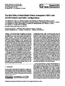
Chemistry module – CHASER
Simulations of atmospheric chemistry in MIROC-ESMCHEM are based on the chemistry model CHASER (Sudo et al., 2002a, 2007) which has been developed mainly at Nagoya University in coorporation with the University of Tokyo, JAMSTEC, and NIES (Fig. 2). The CHASER model version used in MIROC-ESM-CHEM considers the detailed photochemistry in the troposphere and stratosphere by simulating tracer transport, wet and dry deposition, and emissions. The original version of CHASER (Sudo et al., 2002a) focused mainly on tropospheric chemistry, and has been extended to include the stratosphere by incorporating halogen chemistry and related processes. In its present configuration, the model considers the fundamental chemical cycle of Ox -NOx -HOx -CH4 -CO with oxidation of VOCs and halogen chemistry calculating concentrations of 92 chemical species with 262 chemical reactions (58 photolytic, 183 kinetic, and 21 heterogeneous reactions). For VOCs, the model includes oxidation of ethane (C2 H6 ), ethene (C2 H4 ), propane (C3 H8 ), propene (C3 H6 ), butane (C4 H10 ), acetone, methanol, isoprene, and terpenes. The model adopts the condensed isoprene oxidation scheme of P¨oschl et al. (2000) which is based on the Master Chemical Mechanism (MCM, Version 2.0) (Jenkin et al., 1997). Terpene oxidation is largely based on Brasseur et al. (1998). The model also includes detailed stratospheric chemistry, calculating ClOx , HCl, HOCl, BrOx , HBr, HOBr, Cl2 , Br2 , BrCl, ClONO2 , BrONO2 , CFCs, HFCs, and OCS. The formation of PSCs and associated heterogeneous reactions on their surfaces (13 reactions for halogen species and N2 O5 ) are calculated based on the schemes adopted in the CCSR/NIES stratospheric chemistry model (Akiyoshi et al., 2004; Nagashima et al., 2001). The photolysis rates (J-values) are calculated on-line using temperature and radiation fluxes computed in the radiation component of the MIROC-AGCM (Sekiguchi and Nakajima, 2008) considering absorption and scattering by gases, aerosols, and clouds as well as the effect of surface albedo. In MIROC-ESM-CHEM, influences of short-wave radiative forcing associated with the solar cycle, volcanic eruptions, and subsequent changes in stratospheric ozone are also taken into account for the calculation of the photolysis rate. In the original MIROC-AGCM, the wavelength resolution for the radiation calculation is relatively coarse in the ultraviolet and the visible wavelength regions as in general GCMs. www.geosci-model-dev.net/4/845/2011/
851 Therefore, the wavelength resolution in these wavelength regions is improved for the photochemistry in CHASER (see Sect. 2.1.1). In addition, representative absorption crosssections and quantum yields for individual spectral bins are evaluated depending on the optical thickness computed in the radiation component. In a similar manner to Landgraf and Crutzen (1998), we optimized the averaging (weighting) function for each spectral bin differently for the troposphere and stratosphere. The simulated distributions of trace gases are generally well in line with the observations (Sudo et al., 2002b). In the default configuration of the MIROC-ESM-CHEM model, sulfate formation from oxidation of SO2 and DMS is basically simulated in the SPRINTARS model component using concentrations of oxidants (OH, O3 , and H2 O2 ) calculated by the CHASER chemistry. Alternatively, the CHASER model component can simulate sulfate and nitrate aerosols on-line in cooperation with the aerosol thermodynamics model ISORROPIA (Nenes et al., 1998; Fountoukis et al., 2007) by considering the ammonia chemistry. It should be noted that sulfate simulation in CHASER considers neutralization of acidity of cloud water by ammonium and dust cations and its influences on liquid phase oxidation of S(IV) to form sulfate, but such processes are not included in the SPRINTARS sulfate simulation (which assumes a constant pH value for cloud water). The latest version of CHASER also includes chemical formation of secondary organic aerosol (SOA) from oxidation of VOCs (isoprene, terpenes, and aromatics) with a “two product” scheme based on Odum et al. (1996). However, our present experiments for the CMIP5 and related projects do not use this on-line SOA simulation mainly because it is yet to be adequately validated. The spatial and temporal resolutions for the chemistry and aerosol calculations are linked to the main dynamical and physical cores of the model (MIROC-AGCM), and grid/subgrid scale tracer transport is simulated in the framework of the GCM. For the CMIP5 related experiments, surface and aircraft emissions of BC/OC and precursor gases (NOx , CO, VOCs, and SO2 ) are specified from the RCP database (Lamarque et al., 2010, etc.). Lightning NOx emission, calculated in the convection scheme of the MIROC-AGCM, is changeable from year to year responding to the interannual variability and climatic trends. Although MIROC-ESMCHEM includes the land surface model MATSIRO and the land ecosystem model SEIB-DGVM, biogenic emissions of VOCs, such as isoprene or terpenes, are not curently linked to the vegetation processes in these models. 2.2
Ocean and sea-ice model with biogeochemistry
The ocean component of MIROC-ESM is developed at CCSR, University of Tokyo, and is called COCO, the acronym of CCSR Ocean COmponent model. The COCO Geosci. Model Dev., 4, 845–872, 2011
852
S. Watanabe et al.: MIROC-ESM 2010
1 Figure 2. Coupling of chemistry calculations (based on models) the CHASER and Fig. 2. 2Coupling of chemistry and aerosol calculations and (basedaerosol on the CHASER and SPRINTARS in the MIROC-ESM-CHEM modeling framework. Note that SOA production from VOCs and nitrate aerosol (NO− ) are considered in the CHASER 3 framework. Note that SOAcomponent in 3 SPRINTARS models) in the MIROC-ESM-CHEM modeling cooperation with the aerosol thermodynamics module ISORROPIA, but are not included in the simulation for the CMIP5 and other related experiments. 4 production from VOCs and nitrate aerosol (NO3-) are considered in the CHASER component 5
in cooperation with the aerosol thermodynamics module ISORROPIA, but are not included in
solves the primitive equations under hydrostatic and Boussicarbon and calcium flow. The sea-air CO2 flux is calculated 6 the simulation for the CMIP5 and other related experiments. nesq approximations with an explicit free surface. The surby multiplying the difference of ocean-atmosphere CO2 parface mixed tial pressures by the ocean gas solubility. 7 layer parameterization is based on Noh and Kim’s turbulence closure scheme (Noh and Kim, 1999), a deriva2.3 Land surface models tive of Mellor and Yamada level 2.5 (Mellor and Yamada, 1982). The sea-ice is based on a two-category thickness 2.3.1 Physical land component – MATSIRO representation, zero-layer thermodynamics (Semtner, 1976), and dynamics with elastic-viscous-plastic rheology (Hunke MIROC-ESM includes a land surface model: Minimal Adand Dukowicz, 1997). vanced Treatments of Surface Interaction and RunOff (MATThe horizontal resolution for COCO is finer than for the SIRO; Takata et al., 2003), coupled to a river routing model, atmospheric model. The longitudinal grid spacing is about TRIP (Oki and Sud, 1998), for calculating river discharge. In 1.4 degrees, while the latitudinal grid intervals gradually MATSIRO, the heat and water exchanges between the land vary from 0.5 degrees at the equator to 1.7 degrees near and atmosphere are calculated, as are the thermal and hydrothe North/South Pole. The vertical coordinate is a hybrid logical conditions in the soil. The model consists of a single of sigma-z, resolving 44 levels in total: 8 sigma-layers near layer canopy, three layers of snow, and six layers of soil to a the surface, and 35 z-layers at depth, plus one bottom layer depth of 14 m. for the boundary parameterization (K-1 model developers, The aging effect on snow albedo (Yang et al., 1997) has 2004). been applied to MATSIRO. The effects of dirt in snow had A simple biogeochemical process is employed to simubeen considered as a constant after Yang et al. (1997), but late the ocean ecosystem. A type of Nutrient-Phytoplanktonwas modified to vary in accordance with the dirt concentraZooplankton-Detritus model (NPZD, Oschlies, 2001) is suftion at the snow surface to mimic the observed relation beficient to resolve the seasonal variation of oceanic biologitween snow albedo and dirt concentration (Aoki et al., 2006). cal activities at a basin-wide scale (Kawamiya et al., 2000). The dirt concentration in snow is calculated from the deposi45 The biological primary production and NPZD variables are tion fluxes of dust and soot calculated in the aerosol module, computed above the euphotic layer, in a nitrogen-base. A SPRINTARS (Sect. 2.1.2). Since the absorption coefficients constant Redfield ratio (C/N = 6.625) is used to estimate the of dust and soot are very different, the relative strength of Geosci. Model Dev., 4, 845–872, 2011
www.geosci-model-dev.net/4/845/2011/
S. Watanabe et al.: MIROC-ESM 2010 their absorption (0.012 for soil dust and 0.988 for black carbon) are weighted to the deposition fluxes to obtain a radiatively effective amount of dirt in snow. The surface albedo of an ice sheet had been assumed to be constant, but has been modified to consider the effects of melt water on the surface (Bougamont et al., 2005). Here, the ice sheet albedo is a function of the water content above the ice for visible and near-infrared radiation, and is a fixed value of 0.05 for the infrared band. 2.3.2
Land ecosystem model – SEIB-DGVM
The process-based terrestrial ecosystem model SEIB-DGVM (Spatially Explicit Individual-Based Dynamic Global Vegetation Model; Sato et al., 2007; Ise et al., 2009) was coupled to MIROC-ESM to simulate global vegetation dynamics and terrestrial carbon cycling. Under global climate change, terrestrial ecosystems will be affected by aspects including shifts in vegetation types, changes in living biomass, alterations of vegetation structure and energy balance, and accumulation and decomposition of soil organic carbon. These changes will in turn influence the climate, thereby forming a terrestrial-atmosphere feedback. In order to appropriately reproduce these terrestrial ecological processes, SEIB-DGVM adopts an individual-based simulation scheme that explicitly captures light competition among trees, while other terrestrial ecosystem models (e.g. Sitch et al., 2003) rely heavily on parameterization for plant competition. Incorporating ecological realities of competition for light is fundamentally important to strengthen DGVM predictions (Purves and Pacala, 2008). SEIB-DGVM has been validated in various regions with different biomes (Ise and Sato, 2008; Sato, 2009; Sato et al., 2010). In this model, the ecological processes – ecophysiology, population, community, and ecosystem dynamics – are simulated in an integrated manner. In SEIB-DGVM, vegetation is classified into 13 plant functional types (PFTs), consisting of 11 tree PFTs and 2 grass PFTs. Each PFT has different ecophysiological parameters such as maximum photosynthetic rates, optimal temperatures for photosynthesis, and minimum temperatures for frost-related mortality. Allometry relationships and carbon allocation patterns also differ, resulting in differential growth patterns and competition among PFTs under the environmental conditions in each grid cell. Photosynthesis is calculated daily as a function of air temperature, photosynthetically active radiation, and atmospheric CO2 concentration, and modified by air humidity through stomatal control and soil moisture availability. Plant respiration is controlled by the volume of plant tissues (i.e. leaves, stems, and root), growth rates of each tissue, and air temperature with a Q10 function. Population dynamics (establishment, growth, and mortality) and community dynamics (competition and succession) are then simulated from the daily gain from photosynthesis by each tree.
www.geosci-model-dev.net/4/845/2011/
853 Dynamics of soil organic carbon is determined by inputs (turnover of plant tissues and mortality) and the output (decomposition by heterotrophic respiration). Heterotrophic respiration responds linearly to the soil water content and exponentially to the soil temperature via an Arrhenius-type equation. SEIB-DGVM in MIROC-ESM contains two soil organic carbon pools (fast- and slow-decomposing) based on the Roth-C scheme (Coleman and Jenkinson, 1999). The ecosystem carbon balance is then calculated by adding changes in living biomass and soil organic carbon. In order to represent the effects of anthropogenic land use change, SEIB-DGVM incorporates land use datasets of RCPs scenarios (Hurtt et al., 2009) for the period 1500–2100. The spatial resolution of the datasets is converted to T42 and land use types are summarized into five categories: primary vegetation, secondary vegetation, pasture, cropland, and urban area. Transitions are reproduced by a dataset of fractional changes of land use area in each grid of MIROC-ESM and computed using an annual time step. The secondary vegetation is formed as a result of logging or burning of primary forests or abandonment of agricultural land. Regrowth of forest PFTs is then simulated by the individual-based forest dynamics scheme. Carbon in harvested biomass is transferred into carbon pools of linear decay (with turnover times of 1, 10, and 100 yr) according to the Grand Slam Protocol described in Houghton et al. (1983). We simulate the ecosystem dynamics of agricultural land using the processes for natural grassland, but the biomass of cropland is harvested annually and partly transferred into the grand slam carbon pools. The anthropogenic land use changes alter the vegetation structure and carbon cycle in terrestrial ecosystems, and resultant changes of land surface conditions and atmospheric CO2 will affect the climate through biophysical/biogeochemical processes.
3 3.1
Spin-up and experimental designs Spin-up and initial condition
Figure 3 schematically illustrates the spin-up procedures of MIROC-ESM. The terrestrial and ocean carbon cycles require a long time to reach equilibrium compared to physical climate systems. In our approach, the terrestrial carbon cycle component including the vegetation dynamics (SEIBDGVM) and the ocean carbon cycle component embedded in the ocean GCM were separately spun-up for 2000 and 1245 yr, respectively (Fig. 3a). In these first off-line spinup runs, surface physical quantities such as winds, temperature, moisture, precipitation, and radiation flux, which are the year-round daily climatology of a pre-industrial run of MIROC, were recursively adapted to each model. Next, we inputted the resultant equilibrated carbon cycle data into a low-top version of MIROC-ESM, in which the L80-AGCM is replaced by a L20-AGCM for computational efficiency, as Geosci. Model Dev., 4, 845–872, 2011
854
S. Watanabe et al.: MIROC-ESM 2010 Ocean Climate + Biogeochemistry
(a) off-line COCO+NPZD 1245yr (b) on-line (c) off-line (d) on-line (e) on-line
Land Biogeochemistry + Biogeography SEIB-DGVM 2000yr
low-top MIROC-ESM 200yr SEIB-DGVM 4350yr low-top MIROC-ESM 180yr MIROC-ESM 100yr
Fig. 3. Spin-up procedures of MIROC-ESM.
initial conditions, and the on-line terrestrial and ocean carbon cycles were integrated for 200 yr (Fig. 3b). The resultant terrestrial carbon cycle state was again input into the off-line SEIB-DGVM, which was integrated for 4350 yr to adapt to the land-use corresponding to 1850 (Fig. 3c). Using the terrestrial carbon cycle data, the second on-line spin-up was conducted using the low-top MIROC-ESM for 180 yr (Fig. 3d), from which the final states of carbon cycle are used as the initial conditions for the final on-line spin-up of MIROC-ESM with the L80-AGCM (Fig. 3e). In the course of the spin-up runs, we monitored representative states and fluxes in the physical climate and carbon cycle components, for example, surface air temperatures, radiation fluxes at the top of atmosphere, strength of the thermohaline circulation, sea-ice extent, soil and vegetation carbon storage, land and ocean carbon uptakes, and so many. Each of the spin-up runs was continued until linear trends of those quantities in the last 50 yr became insignificant. After the spin-up had finished, we conducted the pre-industrial control run of MIROC-ESM for 530 yr, and the first day of the 20th year of the control run was used as the initial condition of the chemistry coupled spin-up of MIROC-ESM-CHEM, which is described in the next paragraph. The atmospheric chemistry component (CHASER) of MIROC-ESM-CHEM was spun-up separately from the carbon cycles because the atmospheric chemistry does not need thousands of years to reach equilibrium. Some chemical species important in the stratosphere required a few tens of years to reach equilibrium if the surface emission of source gases was substantially changed. Since we had only run the current version of CHASER under present-day conditions before CMIP5, we first needed to prepare appropriate initial conditions for 1850 utilizing the existing presentday dataset: (1) concentrations of halogen compounds such as halocarbons, inorganic chlorine and bromine were set to zero, (2) concentrations of the nitrogen family such as nitrogen dioxide was scaled on the basis of present-day values Geosci. Model Dev., 4, 845–872, 2011
with reference to the surface concentration of nitrous oxide, and (3) concentration of methane and moisture were scaled with reference to the surface concentration of methane. After a spin-up of about 15 yr, the concentrations of all chemical compounds in the troposphere and stratosphere reached equilibrium. The chemistry spin-up run was continued for 28 yr, and the final states of the chemistry tracers were added to the initial condition of the carbon cycles described in the previous paragraph. Finally, a fully-coupled carbon cycles-chemistry spin-up run was performed for 4 yr to derive the initial condition of the historical simulation, whose results are described in Sect. 4. This short final spin-up run was possible because: (1) the pre-industrial mean climate of MIROC-ESM that is used for the carbon cycle spin-up and of MIROC-ESMCHEM was actually similar to each other, because ozone distribution in these models is similar. (2) The present version of MIROC-ESM-CHEM does not include any direct coupling between the carbon cycles and atmospheric chemistry. The atmospheric chemistry indirectly affects ecosystems through chemistry-climate interactions. At least, we did not find any apparent changes in ecosystems before and after the chemistry coupling. 3.2
Experimental designs
The historical simulation was performed for the period from 1850 to 2005 using a set of external forcings recommended by the CMIP5 project. Spectral changes in solar irradiance are considered according to Lean et al. (2005). Historical changes in optical thickness of volcanic stratospheric aerosols are given by Sato et al. (1993) and subsequent updates (http://data.giss.nasa.gov/modelforce/strataer/). Unlike our previous simulations, the temporal evolution of the optical thickness in latitude-altitude cross section is considered. From 1998, the optical thickness of volcanic stratospheric aerosols is exponentially reduced with one year relaxation time. In CMIP5 simulations, CHASER and SPRINTARS do not calculate stratospheric background aerosols made from carbonyl sulfide. The optical thickness of volcanic stratospheric aerosols does include the stratospheric background aerosols, and we use it in radiation calculations and heterogeneous chemistry calculations as the optical thickness per unit altitude can be converted into surface area density of aerosols. Atmospheric concentrations of well-mixed greenhouse gases are provided by Meinshausen et al. (2011). Surface emissions of tropospheric aerosols and ozone precursors are provided by Lamarque et al. (2010). To appropriately incorporate the effects of anthropogenic land use, the harmonized land-use dataset (Hurtt et al., 2009) was implemented in the SEIB-DGVM. The harmonized land use dataset provided global land use type transitions among five types (primary vegetation, secondary vegetation, cropland, pasture, and urban area) in fractions annually at a resolution of 0.5 degrees and was prepared by integration www.geosci-model-dev.net/4/845/2011/
S. Watanabe et al.: MIROC-ESM 2010
855
of four RCP socioeconomic studies (IMAGE, MINICAM, AIM, and MESSAGE) and historical data (1500–2005). The original harmonized land-use data were converted to T42 to fit the spatial resolution of this study by taking weighted means. The quality of the conversion was checked graphically. Implementation of RCPs in SEIB-DGVM is described in Sect. 2.3.2. 4 4.1
Results of historical simulation Transient variations
Temporal variations of global and annual mean surface air temperature (SAT) are shown in Fig. 4 for the MIROC-ESMCHEM simulation as well as for the observations (Brohan et al., 2006). The MIROC-ESM-CHEM simulation well captures the observed multi-decadal variations throughout the whole simulation period, although the simulated SAT is about 0.2 ∼ 0.3 K cooler than observations since the Pinatubo eruption. The simulated SAT increase in the first and the second half of the 20th century is about 0.8 and 1.0 K century−1 respectively, which is slightly less than that in the observations. These global annual mean SAT trends are similar to those of our previous simulations (Nozawa et al., 2007), although we use different forcing datasets than previously. Figure 5 shows the geographical distributions of linear SAT trends for the first and second half of the 20th century. For the first half of the 20th century (Fig. 5a and b), the simulated SAT trends are about 1/2 or smaller than observations over the ocean. The simulated SAT trends are positive over Eurasia despite the observed SAT trends are generally negative. For the second half of the 20th century (Fig. 5c and d), on the other hand, the overall SAT trend for the MIROC-ESM-CHEM simulation shows a realistic geographical pattern, as compared to the observed one: the simulated SAT trend pattern over the northern Pacific is very similar to that in observations, although the simulated trends over the Southern Hemisphere are about 1 K century−1 smaller than those in observations. 4.2
Climatology in the late 20th century
Figure 6a and b shows geographical distributions of SAT averaged for the 1961–1990 periods for the MIROC-ESMCHEM simulation and its biases against observational dataset (Jones et al., 1999), respectively. Overall, MIROCESM-CHEM SAT distributions are realistic but their differences from observations show systematic biases: the simulated SAT is warmer in the mid and high latitudes of the Northern Hemisphere and over Antarctica. On the other hand, the simulated SAT is about 1 ∼ 2 K cooler in the tropics and in the mid latitudes of the Southern Hemisphere. The MIROC-ESM-CHEM shows a realistic distribution of annual mean precipitation for the 1981–2000 period (Fig. 6c). However, there are some differences compared www.geosci-model-dev.net/4/845/2011/
Fig. 4. Temporal variations of global annual mean surface air temperature (SAT). Anomalies from the 1851–1900 mean for the observations (Brohan et al., 2006; black line) and the MIROC-ESMCHEM simulation (red line). In calculating the global annual mean SAT, modeled data are projected onto the same resolution as the observations, discarding simulated data at grid points where there was missing observational data. At each location, more than two months of data were required to calculate the seasonal mean value, and all four seasons of data were required to calculate the annual mean value.
with the GPCP observational dataset (Adler et al., 2003) (Fig. 6d): the precipitation is underestimated along the South Pacific convergence zone (SPCZ), over the eastern side of the Maritime Continent, and over Central America, whereas it is overestimated over the Maritime Continent, the northwestern Indian Ocean, and the western side of South America. These shortcomings are similar to those in our previous model (MIROC3.2) because these two models have almost the same atmospheric physics components. There is significant interest in how many years the Arctic and Antarctic sea-ice can last in a warming globe. Supposing a slightly warming ocean, both the sea-ice extent and the surface albedo would decrease and more solar radiation would be absorbed by the ocean, and hence initial warming is accelerated. Therefore, Arctic and Antarctic sea-ice are very sensitive in a changing climate and can provide a good benchmark for a climate model. Figure 7 compares the sea-ice concentration between the reanalysis (Reynolds et al., 2002) and simulation by seasons and hemispheres. MIROC-ESM-CHEM reasonably simulates the sea-ice seasonality in both hemispheres. The sea-ice distribution is similar between the reanalysis and simulation. During the boreal summer (JJA), the Arctic Ocean has less sea-ice and the Southern Ocean has more sea-ice compared with the other seasons, and vice versa for the boreal winter (DJF). However, some unrealistic features can be found in the simulation, especially over shallow oceans. Hudson Bay, for example, has thin sea-ice during the boreal summer in the reanalysis while no sea-ice is formed in the simulation. The Geosci. Model Dev., 4, 845–872, 2011
856
S. Watanabe et al.: MIROC-ESM 2010
(a)
(c)
(b)
(d)
Fig. 5. Geographical distributions of linear surface air temperature trends (K century−1 ) in the (a, b) first and (c, d) second half of the 20th century for the (a, c) observations (Brohan et al., 2006) and (b, d) the MIROC-ESM-CHEM simulation. Trends were calculated from annual mean values only for those grid points where the annual data is available in at least 2/3 of the 50 yr and distributed in time without significant bias.
southwestern Okhotskoe Sea and northern Barrentsovo Sea also have less sea-ice during the boreal winter in the simulation. Therefore, MIROC-ESM-CHEM underestimates a small amount of sea-ice over shallow oceans and such sea-ice may have disappeared by the 1990s, a bit earlier than in the observations, but the model adequately resolves most other sea-ice, which has more importance in a large-scale climate simulation. The annual mean shortwave (SW) and longwave (LW) radiation at the top of the atmosphere (TOA), and their cloud radiative forcing (CRF) are shown in Figs. 8 and 9. The observational dataset from the Earth Radiation Budget Experiment (ERBE), Earth Radiant Fluxes and Albedo for Month S-9 for the period 1986 to 1990 (Barkstrom et al., 1989) is used for comparison with the model simulation. As shown in Fig. 8, negative bias in SW radiation (the model has too much reflection) and CRF can be seen in the central Pacific, western Atlantic, and Indian Ocean, and positive bias is seen in the eastern Pacific and Atlantic. These features are similar to the bias of low-level cloud albedo in Fig. 12 of Yokohata et al. (2010), and thus these biases are likely caused by the model feature of low-level cloud. As for LW radiation, the bias is relatively small compared to that in SW radiation. A positive bias in LW radiation and LW CRF can be seen over the intertropical convergence zone (ITCZ) in the equatorial Pacific. Since this feature is similar to that of the precipitation bias shown in Fig. 6d, Geosci. Model Dev., 4, 845–872, 2011
this positive bias in LW radiation is likely caused by a problem with the model precipitation or convection. Similarly, the negative bias in the LW radiation and LW CRF over the SPCZ may be related to the negative precipitation bias there (Fig. 6d). The meridional cross sections of simulated zonal mean temperatures, specific humidity, and relative humidity are shown in Fig. 10, along with those biases against ERA-40 (Uppala et al., 2005). A cold bias is seen near the surface except in the Arctic. This is consistent with that in SAT (Fig. 6b). At higher altitudes, a cold bias is seen in the middle troposphere between 40◦ N and 50◦ S, and a larger cold bias is seen in the extratropical upper troposphere and lower stratosphere. A large negative (dry) bias is seen in the lower troposphere, especially at latitudes lower than 30 degrees. Reasons for the dry bias in these regions are related to the cold bias near the surface (Fig. 10b) and the dry bias in the relative humidity centered around 850 hPa (Fig. 10d). In the region where the dry bias in relative humidity is maximal, the dry bias in specific humidity is also maximal. In the upper troposphere and lower stratosphere, a large positive (wet) bias in relative humidity is seen. This bias could cause the negative temperature bias (Fig. 10b) owing to an increase in LW emission to outer space. The meridional cross sections of simulated zonal mean eastward winds and temperatures are shown in Fig. 11, along www.geosci-model-dev.net/4/845/2011/
S. Watanabe et al.: MIROC-ESM 2010
857
Fig. 6. (a) Annual mean climatology of surface air temperature (SAT) for the 1961–1990 period for the MIROC-ESM-CHEM simulations and (b) biases in the annual mean SAT climatology against the observational dataset (Jones et al., 1999). (c) Annual mean climatology of precipitation for the 1981–2000 period for the MIROC-ESM-CHEM simulations and (d) biases in the annual mean precipitation climatology against the GPCP observational dataset (Adler et al., 2003).
with those for ERA-40 (below 1 hPa) and the 1986 Committee on Space Research (COSPAR) International Reference Atmosphere (CIRA) data (above 1 hPa) (Fleming et al., 1990). The model qualitatively reproduces the observed meridional structure of the zonal mean winds and temperatures in each month (January, April, July, and October). Relatively large discrepancies between the model and observations are found in the winter hemisphere high latitudes. More frequent occurrence of stratospheric sudden warming than that in the observations in the 1990s results in weak winds in the northern winter upper stratosphere and mesosphere (Fig. 11a). Less gravity wave drag owing to a lack of lateral propagation in gravity wave drag parameterizations causes strong winds in the southern winter upper stratosphere and mesosphere (Fig. 11e, see Watanabe, 2008). Figure 12 compares time-height cross-sections for the reanalysis (ERA-40) and simulated equatorial eastward winds. They both show alternation of downward propagating eastward and westward wind shear zones, known as the equatorial QBO. The mean periods of the observed and simulated QBO are similar to each other, i.e. approximately 28 months, while the simulated QBO behavior is somewhat www.geosci-model-dev.net/4/845/2011/
regular compared to the reanalysis. This might be due to the constant gravity wave source specified in the tropics (Sect. 2.1.1). Otherwise, it could be attributed to less variability of resolved wave forcing and/or of the equatorial mean upward motions. The QBO in MIROC-ESM will be detailed in a forthcoming paper (Watanabe and Kawatani, 2011). 4.3
Aerosols
Significant changes in atmospheric aerosol loading from preindustrial times to the present result from industrial activities and biomass burning (Fig. 13). BC, OM, and sulfate from anthropogenic sources are emitted from East and South Asia, North America, and Europe and then transported to the outflow regions. They also originate from biomass burning caused by deforestation in Southeast Asia, central and southern Africa, and the Amazon. Figure 14 shows the time evolution of the global mean increasing rate of mass column loading for each aerosol component. BC and sulfate gradually increased after the Industrial Revolution to the first half of the 20th century mainly due to consumption of fossil fuel, and then accelerated after 1950s along with OM due Geosci. Model Dev., 4, 845–872, 2011
858
S. Watanabe et al.: MIROC-ESM 2010
Fig. 7. Seasonal climatology of Arctic and Antarctic sea-ice concentration in the 1990s: for the boreal (JJA) and austral (DJF) summer, and the reanalysis (OISST) and simulation (MIROC-ESM-CHEM).
to rapid industrialization and deforestation. Global mean aerosol mass in the atmosphere at the end of the 20th century is about three times and twice as large as that in 1850 for BC and sulfate, respectively. Atmospheric dust slightly increased in the 20th century relative to the previous century. Anthropogenic aerosols from urban areas in the mid-latitudes of the Northern Hemisphere concentrate in the boundary layer, while biomass burning aerosols from tropical and subtropical regions are injected to higher altitudes due to convection and fire heat (Fig. 15). Figure 16 shows the direct radiative forcing at the tropopause due to anthropogenic aerosols under all-sky condition, which have strong negative values over industrialized and biomass burning regions. The radiative forcings of the direct and indirect effects due to anthropogenic aerosols are −0.2 W m−2 and −0.9 W m−2 for the global mean, respectively. 4.4
Atmospheric chemistry
Figure 17 displays the temporal evolution of the global mean ozone column reproduced by our past simulation with MIROC-ESM-CHEM using the RCP dataset for CMIP5. The total ozone column rapidly decreases after 1980 in response to the increased halogen loading, exhibiting the large influence of volcanic eruptions in 1980s and 90s. The decreasing trend of total ozone in 1980s, however, appears to Geosci. Model Dev., 4, 845–872, 2011
be significantly underestimated by the model in view of the long-term trend in stratospheric ozone observed during this time period (about −1 % yr−1 ) (e.g. World Meteorological Organization (WMO), 2007). In comparison with the total ozone measurements by the total ozone mapping spectrometer (TOMS), we found an overestimation (5–10 %) by the model in the low to midlatitudes through a year with a less overestimation (