Missing Values in Hierarchical Nonlinear Factor ... - Semantic Scholar
Recommend Documents
it reconstructs missing values in observations. The. NFA model uses ... speech data and Boston housing data, we conclude that the ... Generative models handle missing values in an easy ..... and nd principal components and in the middle the.
Atlantic University-Sea Tech, Dania Beach, FL 33004-3023 USA (e-mail: [email protected]). W. M. Haddad is with the School of Aerospace Engineering,.
you do calculations using Excel statistical functions, eg ... You can replace “” in
the “if” formula with na() eg =if(isnumber(cell),log(cell),na()). Note that if you copy
...
May 1, 2017 - ... Sara Crawford, Sheree Boulet, Michael Monsour, Bruce Cohen, Patricia McKane, and Karen ..... Grigorescu, V., Zhang, Y., Kissin, D., et al.
Jan 29, 2015 - Agr family includes three groups of genes, Ag1, Agr2 and Agr3, which encode ... By contrast, higher vertebrates have only Agr2 and Agr3, but.
that methods 4,9 perform very well among all nine methods. For this reason we adopt these methods in this work for the treatment of missing values and they.
input data, to select the best patterns and variables for the training and to fill missing values. On the other hand, statistical data analysis techniques [3, 7, 12, 19, ...
Breast Cancer Data Analytics With Missing Values: A study on Ethnic, Age and Income Groups. Santosh Tirunagariâ, Norman Pohâ , Hajara Abdulrahmanâ¡, ...
Michael R. Berthold and Klaus{Peter Huber. Institute for Computer Design and Fault Tolerance (Prof. D. Schmid). University of Karlsruhe, Am Zirkel 2, 76128 ...
Keywords: Data envelopment analysis; Missing values; Interval DEA. 1. .... In such a setting, the units are free to assign any value within the intervals so as to ...
Further modifications of the SOM using k-nearest neighbor calculations result in lower classification errors and lower variances of classification errors.
IOS Press, 2003. A Methodology for ... notifications from two distinct patients, also called homonym errors, and failure to link multiple notifications on the same ...
Romano (1995), and the matched-block bootstrap of Carlstein et al. (1998) .... Second, define blocks of 1 consecutive observations Yi,n = (Xi,n, ... ,XHI-1,n).
on the predictive variables. library(breedR). N
and McKinley [15] choose tiles based on cache parameters to re- duce self- ..... the Kendall Square Research KSR-1 and the Stanford DASH multiprocessors. In.
Our study utilized the instance-based classifier implemented in Weka [8] to ... Imputation of missing software engineering metrics data and its associated ...
Several subnets were trained, each with one of the ... missing inputs the subnets were trained to classify the ... However in practice, it was found useful to perform.
can deal with them. Missing data is a familiar and unavoidable problem in large datasets and is widely discussed in the field of data mining and statistics.
Monotone troubles appear in various domain areas like credit rating, bankruptcy prediction, bond rating etc. It can thus
May 7, 2010 - of (non missing) observations (e.g. Koutsoyiannis and Langousis, 2010). ... or of dry years to cluster into drought periods (e.g. Koutsoyiannis,.
Milan Jovovic a, Slavica Jonic a,b, Dejan Popovic a,b,* ... E-mail address: [email protected] (D. Popovic) ...... [9] Pitas I, Milos E, Venetsanopoulos AN.
fier composed of several artificial neural networks (ANN's) organised in a tree-like .... Rule extraction from trained ANN's algorithm is based on FERNN â Fast Ex-.
Dec 22, 2011 - Email: [email protected], [email protected], ... Broadcast Channel, Hierarchical Modulation, Digital Video Broadcasting. ... In superposition coding, the available energy is shared to several service flows which are sent ...
Missing Values in Hierarchical Nonlinear Factor ... - Semantic Scholar
For a more detailed discussion, see [9]. The missing values in data behave like other latent variables and are therefore seen as a part of θ. Re- constructing ...
MISSING VALUES IN HIERARCHICAL NONLINEAR FACTOR ANALYSIS ¨ Tapani Raiko, Harri Valpola, Tomas Ostman and Juha Karhunen Helsinki University of Technology, Neural Networks Research Centre P.O. Box 5400, FIN-02015 HUT, Espoo, Finland [email protected] http://www.cis.hut.fi/projects/ica/bayes/ ABSTRACT The properties of hierarchical nonlinear factor analysis (HNFA) recently introduced by Valpola and others [1] are studied by reconstructing missing values. The variational Bayesian learning algorithm for HNFA has linear computational complexity and is able to infer the structure of the model in addition to estimating the parameters. To compare HNFA with other methods, we continued the experiments with speech spectrograms in [2] comparing nonlinear factor analysis (NFA) with linear factor analysis (FA) and with the self-organising map. Experiments suggest that HNFA lies between FA and NFA in handling nonlinear problems. Furthermore, HNFA gives better reconstructions than FA and it is more reliable than NFA. 1. INTRODUCTION A typical machine learning task is to estimate a probability distribution in the data space that best corresponds to the set of real valued data vectors x(t) [3]. This probabilistic model is said to be generative - it can be used to generate data. Instead of finding the distributions directly, one can assume that sources s(t) have generated the observations x(t) through a (possibly) nonlinear mapping f (·): x(t) = f [s(t)] + n(t) ,
(1)
where n(t) is additive noise. Principal component analysis and independent component analysis are linear examples, but we focus on nonlinear extensions. It is difficult to visualise the situation if for instance a 10-dimensional source space is mapped to form a nonlinear manifold in a 30-dimensional data space. Therefore, some indirect measures for studying the situation are useful. We use real-world data to make the experiment setting realistic and mark parts of the data to This research has been funded by the European Commission project BLISS, and the Finnish Center of Excellence Programme (2000–2005) under the project New Information Processing Principles.
be missing for the purpose of controlled comparison. By varying the configuration of the missing values and then comparing the quality of their reconstructions, we measure different properties of the algorithms. Generative models handle missing values in an easy and natural way. Whenever a model is found, reconstructions of the missing values are also obtained. Other methods for handling missing data are discussed in [4]. Reconstructions are used here to demonstrate the properties of hierarchical nonlinear factor analysis (HNFA) [1] by comparing it to nonlinear factor analysis (NFA) [5], linear factor analysis (FA) [6] and to the selforganising map (SOM) [7]. Similar experiments using only the latter three methods were presented in [2]. FA is similar to principal component analysis (PCA) but it has an explicit noise model. It is a basic tool that works well when nonlinear effects are not important. The mapping f (·) is linear and the sources s(t) have a diagonal Gaussian distribution. Large dimensionality is not a problem. The SOM can be presented in terms of (1), although that is not the standard way. The source vector s(t) contains discrete map coordinates which select the active map unit. The SOM captures nonlinearities and clusters, but has difficulties with data of high intrinsic dimensionality and with generalisation. 2. VARIATIONAL BAYESIAN LEARNING FOR NONLINEAR MODELS Variational Bayesian (VB) learning techniques are based on approximating the true posterior probability density of the unknown variables of the model by a function with a restricted form. Currently the most common technique is ensemble learning [8] where Kullback-Leibler divergence measures the misfit between the approximation and the true posterior. It has been applied to ICA and a wide variety of other models (see [1, 9] for some references). In ensemble learning, the posterior approximation q(θ) of the unknown variables θ is required to have a
Q suitably factorial form q(θ) = i qi (θ i ), where θi are the subsets of unknown variables. The misfit between the true posterior p(θ | X) and its approximation q(θ) is measured by Kullback-Leibler divergence. An additional term − log p(X) is included toRavoid calculation of the model evidence term p(X) = p(X, θ)dθ. The cost function is q(θ) C = D(q(θ) k p(θ|X)) − log p(X) = log , p(X, θ) (2) where h·i denotes the expectation over distribution q(θ). Note that since D(q k p) ≥ 0, it follows that the cost function provides a lower bound for p(X) ≥ exp(−C). For a more detailed discussion, see [9]. The missing values in data behave like other latent variables and are therefore seen as a part of θ. Reconstructing missing values corresponds to finding the posterior distribution of them given the observed data X. Therefore, the posterior approximation q(θ) can be used directly. The number of missing values does not affect computational complexity substantially. Beal and Ghahramani [10] compare the VB method of handling incomplete data to annealed importance sampling (AIS). In their example, the variational method works more reliably and about 100 times faster than AIS. Chan et al. [11] used ICA with VB learning successfully to reconstruct missing values. A competing approach without VB by Welling and Weber [12] has an exponential complexity w.r.t. the data dimensionality. ICA can be seen as FA with a non-Gaussian source model. Instead of going into that direction, we choose to stick to the Gaussian source model and concentrate on extending the mapping to be nonlinear instead. 2.1. Nonlinear factor analysis and hierarchical nonlinear factor analysis In [5], a nonlinear generative model (1) was estimated by ensemble learning and the method was called nonlinear factor analysis (NFA). A more recent version with an analytical cost function and a linear computational complexity, is called hierarchical nonlinear factor analysis (HNFA) [1]. In many respects HNFA is similar to NFA. The posterior approximation, for instance, was chosen to be maximally factorial for the sake of computational efficiency and the terms qi (θi ) were restricted to be Gaussian. In NFA, a multi-layer perceptron (MLP) network with one hidden layer was used for modelling the nonlinear mapping f (·): f (s(t); A, B, a, b) = A tanh[Bs(t) + b] + a ,
(3)
where A and B are weight matrices, a and b are bias vectors and the activation function tanh operates on
each element separately. The key idea in HNFA is to introduce latent variables h(t) before the nonlinearities and thus split the mapping (3) into two parts: h(t) = x(t) =
Bs(t) + b + nh (t) Aφ[h(t)] + Cs(t) + a + nx (t) ,
(4) (5)
where nh (t) and nx (t) are Gaussian noise terms and the nonlinearity φ(ξ) = exp(−ξ 2 ) again operates on each element separately. Note that we have included a short-cut mapping C from sources to observations. This means that hidden nodes only need to model the deviations from linearity. Learning is unsupervised and thus differs in many ways from standard backpropagation. Each step in learning tries to minimise the cost function (2). In NFA, the sources are updated while keeping the mapping constant and vice versa. The computational complexity is propotional to the number of paths from sources to the data, i.e. the product of sizes of the three layers. In HNFA, all terms qi (θi ) of q(θ) are updated one at a time. The computational complexity is linear with the number of connections in the model and thus HNFA scales better than NFA. In both algorithms, the update steps are repeated for several thousands of times per parameter. In NFA, neither the posterior mean nor the variance of f (·) over q(θ) can be computed analytically. The approximation based on Taylor series expansion may be inaccurate if the posterior variance for the input of the hidden nodes grows too large. This may be the source of the instability observed in some simulations. Preliminary experiments suggest that it may be possible to fix the problem at the expence of efficiency. In HNFA, the posterior mean and variance of the mappings in (4) and (5) have analytic expressions. This is possible at the expense of assuming independencies of the extra latent variables h(t) in the posterior approximation q(θ). The assumption increases the misfit between the approximated and the true posterior. Minimisation of (2) pushes the solution in a direction where the misfit would be as small as possible. In [13], it is shown how this can lead to suboptimal separation in linear ICA. It is difficult to analyse the situation in nonlinear models, but it can be expected that models with fewer simultaniously active hidden nodes and thus more linear mappings are favoured. This should lead to conservative estimates of the nonlinearity of the model. Since HNFA is built from simple blocks introduced in [14], learning the structure1 becomes easier. The 1 By structure, we mean the sizes of the layers and the connections between the nodes. In principle, we could allow any directed acyclic graph connecting the latent and observed variables.
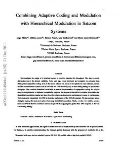
Nonlinearity (patches)
Data with missing values
1.
2.
3.
4.
Generalisation Original data
Memorisation (permuted)
High dimensionality
HNFA reconstruction
Fig. 1. Some speech data with and without missing values and the reconstruction given by HNFA. cost function (2) relates to the model evidence p(X | model) and can thus be used to compare structures. The model is built in stages starting from linear FA, i.e. HNFA without hidden nodes. See [1] for further details. 3. EXPERIMENTS The goal is to study nonlinear models by measuring the quality of reconstructions of missing values. The data set consists of speech spectrograms from several Finnish subjects. Short term spectra are windowed to 30 dimensions with a standard preprocessing procedure for speech recognition. It is clear that a dynamic2 source model would give better reconstructions, but in this case the temporal information is left out to ease the comparison of the models. Half of the about 5000 samples are used as test data with some missing values. Missing values are set in four different ways to measure different properties of the algorithms (Figure 2): 1. 38 percent of the values are set to miss randomly in 4 × 4 patches. (Figure 1) 2. Training and testing sets are randomly permuted before setting missing values in 4 × 4 patches as in Setting 1. 3. 10 percent of the values are set to miss randomly independent of any neighbours. This is an easier setting, since simple smoothing using nearby values would give fine reconstructions. 2 In [9], NFA was extended to include a model for the dynamics of the sources. A similar extension for HNFA would lead to hierarchical nonlinear dynamical factor analysis.
Fig. 2. Four different experimental settings with the speech data used for measuring different properties of the algorithms. 4. Training and testing sets are permuted and 10 percent of the values are set to miss independently of any neighbours. We tried to optimise each method and in the following, we describe how we got the best results. The SOM was run using the SOM Toolbox with long learning time, 2500 map units and random initialisations. One parameter, the width of the softening kernels that was used in making the reconstruction, was selected based on the results, which is not completely fair. In other methods, the optimisation was based on minimising the cost function (2) or its approximation. NFA was learned for 5000 sweeps through data using a Matlab implementation. Varying number of sources were tried out and the best ones were used as the result. The optimal number of sources was around 12 to 15 and the size used for the hidden layer was 30. A large enough number should do, since the algorithm can effectively prune out parts that are not needed. Some runs with a higher number of sources were good according to the approximation of the cost function (2), but a better approximation of the cost function or a simple look at the reconstruction error of the observed data showed that those runs were actually bad. These runs and the ones that diverged were filtered out. The details of the HNFA (and FA) implementation can be found in [1]. In FA, the number of sources was 28. In HNFA, the number of sources at the top layer was varied and the best runs according to the cost function were selected. The size of the top layer varied from 6 to 12 and the size of the middle layer, which is determined during learning, turned out to vary from 12 to 30. HNFA was run for 5000 sweeps through data. Each run with NFA or HNFA takes about 8 hours of processor time, while FA and SOM are faster. Several runs were conducted with different random initialisations but the same data and the same missing value pattern for each setting and for each method. The number of runs in each cell is about 30 for HNFA, 4 for
NFA and 20 for the SOM. FA always converges to the same solution. The mean and the standard deviation of the mean square reconstruction error are:
The order of results of the Setting 1 follow our expectations on the nonlinearity of the models. The SOM with highest nonlinearity gives the best reconstructions, while NFA, HNFA and finally FA follow in that order. The results of HNFA vary the most there is potential to develop better learning schemes to find better solutions more often. The sources h(t) of the hidden layer did not only emulate computational nodes, but they were also active themselves. Avoiding this situation during learning could help to find more nonlinear and thus perhaps better solutions. In the Setting 2, due to the permutation, the test set contains vectors very similar to some in the training set. Therefore, generalisation is not as important as in the Setting 1. The SOM is able to memorise details corresponding to individual samples better due to its high number of parameters. Compared to the Setting 1, SOM benefits a lot and makes clearly the best reconstructions, while the others benefit only marginally. The Settings 3 and 4, which require accurate expressive power in high dimensionality, turned out not to differ from each other much. The basic SOM has only two intrinsic dimensions3 and therefore it was clearly poorer in accuracy. Nonlinear effects were not important in these settings, since HNFA and NFA were only marginally better than FA. HNFA was better than NFA perhaps because it has more latent variables when counting both s(t) and h(t). To conclude, HNFA lies between FA and NFA in performance. HNFA is applicable to high dimensional problems and the middle layer can model part of the nonlinearity without increasing the computational complexity dramatically. FA is better than the SOM when expressivity in high dimensions is important, but the SOM is better when nonlinear effects are more important. The extensions of FA, NFA and HNFA, expectedly performed better than FA in each setting. HNFA is recommended over NFA because of its reliability. It may be possible to enhance the performance of NFA and HNFA by new learning schemes whereas especially FA is already at its limits. On the other 3 Higher dimensional SOMs become quickly intractable due to exponential number of parameters.
hand, FA is best if low computational complexity is the determining factor. 4. REFERENCES ¨ [1] H. Valpola, T. Ostman, and J. Karhunen, “Nonlinear independent factor analysis by hierarchical models,” in Proc. of the 4th Int. Symp. on Independent Component Analysis and Blind Signal Separation (ICA2003), 2003. To appear. [2] T. Raiko and H. Valpola, “Missing values in nonlinear factor analysis,” in Proc. of the 8th Int. Conf. on Neural Information Processing (ICONIP’01), (Shanghai), pp. 822–827, 2001. [3] C. Bishop, Neural Networks for Pattern Recognition. Clarendon Press, 1995. [4] R. Little and D.B.Rubin, Statistical Analysis with Missing Data. J. Wiley & Sons, 1987. [5] H. Lappalainen and A. Honkela, “Bayesian nonlinear independent component analysis by multi-layer perceptrons,” in Advances in Independent Component Analysis (M. Girolami, ed.), pp. 93–121, Berlin: Springer-Verlag, 2000. [6] A. Hyv¨ arinen, J. Karhunen, and E. Oja, Independent Component Analysis. J. Wiley, 2001. [7] T. Kohonen, Self-Organizing Maps. Springer, 3rd, extended ed., 2001. [8] D. Barber and C. Bishop, “Ensemble learning in Bayesian neural networks,” in Neural Networks and Machine Learning (M. Jordan, M. Kearns, and S. Solla, eds.), pp. 215–237, Berlin: Springer, 1998. [9] H. Valpola and J. Karhunen, “An unsupervised ensemble learning method for nonlinear dynamic statespace models,” Neural Computation, vol. 14, no. 11, pp. 2647–2692, 2002. [10] M. Beal and Z. Ghahramani, “The variational Bayesian EM algorithm for incomplete data: with application to scoring graphical model structures,” Bayesian Statistics 7, 2003. To appear. [11] K. Chan, T.-W. Lee, and T. J. Sejnowski, “Handling missing data with variational bayesian estimation of ica,” in Proc. 9th Joint Symposium on Neural Computation, vol. 12, (Institute for Neural Computation, Caltech), May 2002. [12] M. Welling and M. Weber, “Independent component analysis of incomplete data,” in Proc. of the 6th Annual Joint Symposium on Neural Computation (JNSC99), (Pasadena), 1999. [13] A. Ilin and H. Valpola, “On the effect of the form of the posterior approximation in variational learning of ICA models,” in Proc. of the 4th Int. Symp. on Independent Component Analysis and Blind Signal Separation (ICA2003), 2003. To appear. [14] H. Valpola, T. Raiko, and J. Karhunen, “Building blocks for hierarchical latent variable models,” in Proc. 3rd Int. Conf. on Independent Component Analysis and Signal Separation (ICA2001), (San Diego, USA), pp. 710–715, 2001.