Mixture Kalman Filter Based Highway Congestion Mode ... - CiteSeerX

ThA05.1

Proceeding of the 2004 American Control Conference Boston, Massachusetts June 30 - July 2, 2004

Mixture Kalman Filter Based Highway Congestion Mode and Vehicle Density Estimator and its Application Xiaotian Sun, Laura Muñoz, and Roberto Horowitz

Abstract— In this paper, we present our latest results on developing and implementing a traffic congestion mode and vehicle density estimator for a segment of Interstate 210 in Southern California. Using a mixture Kalman filtering (MKF) algorithm on the switching-mode traffic model, the estimator is able to provide estimated vehicle densities at unmeasured locations, as well as the congestion statuses (free-flow or congested), which are not directly observed. The program runs efficiently, thus making it possible to carry out estimation in real time.

I. I NTRODUCTION In today’s metropolitan areas, highway traffic congestion occurs regularly during rush hours. In addition, nonrecurrent congestion often takes place as a result of incidents or road work. The congestion causes inefficient operation of highways, waste of resources, increased air pollution, and intensified driver fatigue. One of the methods used to prevent and/or relieve highway traffic congestion is on-ramp metering. Many strategies have been proposed and deployed to regulate the demands on the highway by limiting the rate at which vehicles enter the highway. These ramp-metering strategies can be classified into two categories: traffic responsive and nontraffic responsive. Traffic responsive ramp metering strategies utilize real-time measurements of the traffic state, such as vehicle densities and traffic congestion status (freeflow or congested), while non-traffic responsive ones often operate under a fixed time-of-the-day table, and ignore the current traffic conditions completely. It is believed that traffic responsive metering strategies are more effective and more robust than non-traffic responsive ones. Currently, traffic data are usually obtained from inductive loop detectors embedded in the pavement. These loop detectors provide percent occupancy (percentage of the time that the detector is occupied by vehicles) and volume (number of vehicles that have passed over the detector), from which other macroscopic quantities can be derived when accurate vehicle lengths are available. These macroscopic quantities include vehicle density (number of vehicles per unit length of highway), flow (number of vehicles per unit time), and speed. One effort to provide such macroscopic traffic data through a centralized database is the Freeway Performance Measurement System (PeMS) [1]. This work has been supported by California Partners for Advanced Transit and Highways (PATH) under Task Order 4136. The authors are with the Department of Mechanical Engineering, University of California at Berkeley, Berkeley, CA 94720-1740. E-mail addresses: {sunx,lmunoz,horowitz}@me.berkeley.edu.

0-7803-8335-4/04/$17.00 ©2004 AACC

Ideally, one would like to have access to these traffic data continuously across time and space. However, because of the high cost and difficulty of installing and maintaining loop detectors, oftentimes traffic data are not available at all desired locations at all times. These missing data thus have to be estimated using the available data. On the other hand, the traffic flow mode, i.e., whether the traffic is in free-flow (where traffic moves freely at high speeds) or congestion (where traffic moves slowly and is restricted by downstream conditions), cannot be measured directly and has to be inferred from other quantities. In our previous work [2], we developed a traffic state estimator based on the switching mode traffic model [3] and the mixture Kalman filter (MKF) [4]. This estimator is able to estimate the vehicle densities at unmeasured locations, as well as to determine the traffic congestion mode, in a highway section. It was tested on a short section of highway and its performance was evaluated using the measured data. It was shown that on average, a mean percentage error of ∼10% was achieved for vehicle density estimation at unmeasured locations. In this paper, we describe our recent work, which involves implementing this congestion mode and vehicle density estimator on our entire selected test site, a 14-mile long segment of Interstate 210 Westbound in Pasadena, California, and interfacing the estimator with traffic simulation programs that have been calibrated to the test segment, including a macroscopic simulator—the modified cell transmission model [5], and a microscopic simulator—VISSIM [6]. We will first briefly review the switching-mode model and the estimation method in Section II. Then in Section III, we will describe the test site and discuss the constraints and other considerations for the cell configuration. The main results will be presented and discussed in Section IV. In the last section, we will give some concluding remarks. II. M ETHOD A. Cell Transmission-Based Switching Mode Model Highway traffic models can be categorized into two groups: microscopic models and macroscopic models. Microscopic models describe the behavior of each individual vehicle on the highway, while macroscopic models describe the evolution of aggregated traffic quantities, such as vehicle densities and flows, based on the conservation principle. Due to their complexity, the microscopic models, which require an enormous number of equations to model each individual vehicle’s behavior and the interaction between

2098

q qm1

qm2 1

2

3

4

QM

β

wc

vf

r

Fig. 3. A schematic plot of a 4-cell highway section with one on-ramp and one off-ramp.

ρ ρc

ρJ

Fig. 1. A trapezoidal fundamental diagram (flow-density relation) used by the cell transmission model. qi

ρi−1

Fig. 2. model.

ρi

A highway section divided into cells in the cell transmission

these vehicles, often can only be solved numerically to simulate the traffic evolution. On the other hand, macroscopic models often consist of a few dynamic equations, along with some constitutional relation between certain traffic quantities, such as the so-called fundamental diagram between flow and density. As an example, a widely used macroscopic model is the Lighthill-Whitham-Richards (LWR) model, which consists of a first-order partial differential equation based on conservation of vehicles, and a flowdensity relationship. Because of their simplicity compared to microscopic models, macroscopic models are often used to quantitatively analyze the effects of changing conditions on traffic behavior. The cell transmission model (CTM) [7], [8] is a macroscopic model. It can be viewed as an approximation and simplification of the LWR model obtained by discretizing the PDE of the LWR model in both space and time, and using a simple trapezoidal fundamental diagram as shown in Fig. 1. The CTM divides a highway into small segments, which are called cells, as shown in Fig. 2. The traffic flow qi going into a cell i is considered constant between two consecutive time points t and t + 1, and is determined by n o
qi (t) = min v f,i−1 ρi−1 (t), wc,i ρ J,i − ρi (t) , Q M,i−1 , (1) where for a cell i, ρi (t) is the average vehicle density between times t and t + 1, ρ J,i is the jam density, i.e., the maximum vehicle density allowed in cell i, v f,i is the free-flow speed, wc,i is the backward congestion wave propagation speed, and Q M,i−1 is the flow capacity, i.e., the maximum possible flow. These quantities are also illustrated in Fig. 1. The three terms involved in the minimum in (1) can be interpreted as follows. The first term v f,i−1 ρi−1 (t) is the flow that can be supplied by cell i−1. The second term is the flow that can be absorbed by cell i. And the third term Q M,i−1

is the maximum possible flow from cell i − 1 to i. Each of these three terms is shown as a thick line segment in Fig. 1 and the minimum is the outline of the trapezoid. Despite the simplifications that are made in the cell transmission model, it still captures many important traffic phenomena, such as queue build-up and dissipation, backward propagation of congestion waves, etc. The simplicity and accuracy of the CTM makes it very desirable for traffic engineering. However, due to the nonlinear nature of the flow-density relationship in the CTM, it can be quite difficult to analyze the model and use it as a basis for designing traffic controllers. Therefore, we have piecewise linearized the CTM and derived a switching-mode model for each section of the highway, based on the traffic congestion status (congested or free-flow) in each section [3]. This switching-mode model includes several modes. In each mode, the vehicle densities in the cells evolve according to a different set of linear difference equations. Among these modes, two are of greatest importance: pure free-flow and full congestion. For the purpose of designing the traffic estimator, we further simplify this switching-mode model by considering only these two modes. For a typical section of highway that consists of 4 cells and contains an on-ramp and an off-ramp, as shown in Fig. 3, we write down this simplified switching-mode model as follows. When the highway section is in free-flow mode, the first term in (1) dominates, and the difference equations are  v T   1 − fl11 s  v f 1 T s ρ1   ρ2  ρ  (t + 1) =  l2 3  0    ρ4 0  Ts  l1 0  +  0 0  0 0 0 0

0 v f 2Ts l2 v f 2Ts l3

1−

0

0

0

0

0

v T 1 − fl33 s v T (1 − β) fl34 s

0 1−

v f 4Ts l4

     ρ1   ρ2     (t)  ρ3   ρ 4

 0     qm1  Ts     l2   qm2  (t) 0   r  0

= A(1)ρ(t) + Bq (1)q(t),

(2) (3)

where qm1 and qm2 are the mainline entering and exiting flows, respectively, r is the on-ramp flow, β is the split ratio of the off-ramp flow, li is the length of cell i, and T s is the sampling time. When the section is in congested mode, the second term

2099

in (1) dominates, and the difference equations are   wc2 T s   0 0 1 − wc1l1T s  ρ  l1 ρ1    1   wc3 T s wc2 T s   ρ2  0 1 − l2 0 ρ2  l 2    (t) ρ  (t + 1) =  wc3 T s 1 wc4 T s    ρ3  0 0 1 − 3   l3 1−β l3    ρ4 wc4 T s  ρ4 0 0 0 1 − l4  Ts  0 0  q  l1     m1  0 0 0  q  (t) +  0 0   m2  0  r Ts 0 − l4 0   wc1 T s − wc2l1T s 0 0  l1  ρ    J1   0 wc3 T s wc2 T s  ρ J2  − 0  l2 l2    , +  wc3 T s w T 1 c4 s   0 0 − 1−β l3  ρ J3  l3  ρ J4  wc4 T s 0 0 0 l4 (4) = A(2)ρ(t) + Bq (2)q(t) + BJ (2)ρ J , (5)

where ρ Ji is the jam density (maximum allowable density) in cell i. It is important to point out that the dynamics of the cell vehicle densities in different modes are dramatically different, as evidenced by the observability and controllability in each mode. In free-flow mode, the densities in the section are observable through a measurement that is downstream of the section and controllable by an on-ramp upstream of the section; while in congestion mode, the densities are observable through a measurement upstream of the section and controllable by an on-ramp downstream of the section. These observations, especially those for congestion mode, are counter-intuitive at a first glance. However they agree with the understanding in highway traffic theory that when during congestion, a high density wave, or in other words, information, propagates backwards along the highway. B. Improved Mixture Kalman Filter In the switching-mode model, the mode (free-flow or congested) is determined by the flow condition in the section. However, there is no direct measurement or observation of the current traffic congestion mode in a highway section. The congestion mode can only be inferred from measured quantities, for example, the speed. The general practice in traffic engineering is to set an upper threshold and a lower threshold for the speed. When the speed in a section is above the upper threshold, the section is considered to be in free flow; when the speed is below the lower threshold, the section is in congestion; when the speed is between the two thresholds, the section is considered somewhat likely to be in congestion. The problem with this kind of method is two-fold: 1) The selection of the thresholds is based on experience and, to a certain degree, is arbitrary, and 2) When the speed falls between the two thresholds, the mode of the section cannot be determined. Therefore, we assume that we do not have direct observation of the mode and that the mode jumps between possible values following a discrete-time Markov chain with a certain transition probability. Under these assumptions,

the switching-mode model falls into a special class, called Markov jump linear systems (MJLS). The previous four-cell example has a continuous state x = [ρ1 ρ2 ρ3 ρ4 ]T and possible discrete modes 1 (free-flow) and 2 (congested). It is known that it is difficult to estimate the states and the mode when the mode itself is not observed. The difficulty lies in the fact that the sample space S t of the mode sequence grows exponentially as time t increases, where S is the set of possible discrete modes. The mixture Kalman filter (MKF) [4] approximately solves this difficult probability inference problem by employing a Monte Carlo approach that approximates the exponentially growing sample space by a fixed finite number, M, of mode sample sequences s(m) t , where m = 1, . . . , M. A weight is associated with each of the sample sequences to represent the a posteriori probability of that sample sequence,   yt , ut p s(m) t (m)  , (6) ξt := P M p s(m) y , u m=1

t

t

t

where a symbol in boldface, for example, st , represents a sequence from time 0 to time t. After the new measurement yt+1 is available, these weights are updated by (m) ξt(m) ζt+1 (m) ξt+1 = P M (m) , (m) m=1 ξt ζt+1

(7)

where the incremental weight   (m) := p yt+1 yt , ut , s(m) ζt+1 , t

(8)

represents the likelihood of the new measurement for a given mode sample sequence. On each of these mode sample sequences, a (timevarying) Kalman filter is implemented to estimate the continuous states. The state estimates on all mode sample sequences are then “mixed” (averaged) by the weights, and this weighted average approximates the a posteriori estimate of the continuous states, i.e., xˆt|t =

M X

(m) ξt(m) xˆt|t ,

(9)

m=1 (m) where xˆt|t is the a posteriori state estimate from each of the Kalman filters. The accuracy of this Monte Carlo method is improved by a predictive sampling technique, in which the current mode is sampled according a predictive probability   µ(m) (s) ∝ p s(m) = s, y s(m) , y , u , (10) t+1

t+1

t+1

t

t

t+1

which favors the mode with higher likelihood given the current measurements and the previously sampled modes. The weight update procedure is recursive. The entire history from time 0 influences the current weight. It is often found in implementation that most of these weights approach 0 while only a few remain of modest magnitudes. This phenomenon reduces the effective number of sample sequences and introduces an underflow risk for

2100

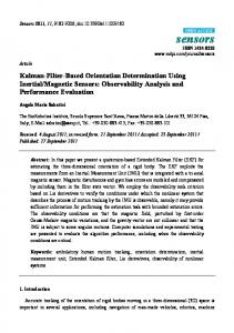
Fig. 4. An aerial photo of the test segment of Interstate 210 Westbound, from Vernon to Fair Oaks, in Pasadena, California (Image source: U.S. Geological Survey digital orthophoto quarter quadrangle, 1996-12-03).

the weights when implemented on a machine with finite floating point precision. Therefore, a forgetting and weight underflow prevention scheme [2] has been introduced in our implementation. In this scheme, the weights of the sample sequences are bounded from below, n (m) o (m) (11) ξt+1 = max ξt+1 ,ξ ,

3) New ramp metering schemes, such as System Wide Adaptive Ramp Metering (SWARM), have undergone testing and evaluation on I-210. 4) District 7 of the California Department of Transportation (Caltrans D7), which manages this highway segment, continues to support researchers in exploring innovative traffic management techniques.

and are re-normalized after the bounding step. This simple procedure not only prevents the underflow, but in effect limits the influence of the early history on the weights and makes the weights recover more quickly when their corresponding sample sequences are favored by the current measurements. In addition to the mixture estimate of the continuous states, the mixture Kalman filter also provides an approximate maximum a posteriori (MAP) estimation of the congestion mode:

Therefore, our efforts in traffic modeling and model calibration have been concentrated on this highway segment.

sˆt,MAP = arg max p (st = s | yt , ut ) , s

where p (st = s | yt , ut ) ≈

M X

  ξt(m) 1 s s(m) , t

(12)

(13)

m=1

and 1 s (st ) is the indicator function. This is particularly important to our application because different control schemes will be used in different congestion modes (free-flow or congested), based on the highway density controllability properties [3]. III. T EST S ITE A segment of Interstate 210 Westbound in Pasadena, California, as shown in an aerial photo in Fig. 4, has been selected as the testbed for new ramp-metering algorithms. It is approximately 14 miles long, from Vernon (Mile Post 39.159) to Fair Oaks (Mile Post 25.4). This site was selected as the preferred test location for the following reasons: 1) It is a heavily used freeway segment that experiences severe recurring congestion and can benefit greatly from ramp-metering strategies that reduce congestion and improve total travel time. 2) I-210 has most of the necessary infrastructure, such as loop detectors, on-ramp metering signal controllers, and a centralized advanced traffic management system (ATMS), that is needed to test new ramp-metering designs.

A. Cell Configuration To apply the switching-mode model to the test highway segment, we first need to divide it into cells. There are several constraints and considerations that we must take into account during this process. 1) The cell transmission model requires that the cell length be larger than the product of the free-flow speed and the time step. In other words, vehicles cannot travel across more than one cell within one time step. 2) With the measurements (density and flow) from mainline loop detectors, the section of highway between two mainline detectors can be decoupled from the rest of the highway. Therefore, we generally divide the highway into sections at the mainline loop detectors. We skip detectors that are believed to be malfunctioning and combine the neighboring sections into one. 3) Within one section, cells are divided at the mergepoints of on-ramps and the diverge-points of offramps. Based on the above considerations, as well as the nominal value of the free-flow speed, 63 miles per hour, the geometry of the highway and the locations of the mainline detectors, we have chosen the sampling time to be 2 seconds. Fig. 5 on the next page shows the cell configuration for the chosen test segment of I-210. In the schematic, the cells are numbered at the corner of each cell, while their lengths, in feet, are marked in the center, in italic typeface. The arrows indicate on- or off-ramps. The entire test segment is divided into 73 cells, and the cells are grouped into 18 sections divided by mainline loop detectors, as shown by thick solid lines in the figure. Some of the mainline loop detectors, shown by thick dashed lines, are not used because they are believed to be malfunctioning.

2101

Travel Direction Vernon 39.159 500

1613.5

73 22

1275

70

1617

462

41 500 40 12

13

265

6

375

8

418.5 10

1284 23

544 24

2

4

815

51

2298

14

50

440

1978

1978

48

14

34

650

1700 62

1100

13

33

975

32

375

46

45

31

1075

1109 1331 300 59 58 57 16 15 18

1456

44

1456

13

15

975

1109 60 17

61 18

19

47

438

625

63 17

30 275

43

1256

12

218

29

14

28 300

535 27

931 21

931

2343

20

825

425

19

625 4

725 16

4

500

3064 13

14

3

6

1975 12 5

4

3 1

1 1

500

8

Fair Oaks 25.4

1000

1

2

7

9

15

5

1450

300

7 5

10

17

6

825

8

688

18

7

650

9,10

9

11

5

7

3

1712 64 18

49

16

525

35

6 4

52

2356 65

19

20

10

360

8

815

1000

22

2350

418.5 9

53 15

1615.5 1615.5 975 37 36 39 38 11 11 12

25

8

475

2356 66

593 67

20

17

544

26

11

54

200

68

21

16

42

550

69

19

55

18

14

937.5

71

21

56

200

1613.5

72

3

2

2

Fig. 5. The cell configuration for the test segment of I-210 West. The cell numbers are marked at the corner of each cell, while the cell length (in feet) are indicated in italic type in the center of each cell. The schematic is not to scale.

IV. R ESULTS AND D ISCUSSION

Mile Post 39.16

38.21

38.07

36.59

35.41

34.9

34.05

33.05

32.2

32.02

31

30.78

30.14

30

29.88

29.17

28.27

28.03

26.8

26.12

25.68

25.4

5

61.64

66.01

63.88

59.76

60.87

60.28

60.43

61.10

61.87

62.28

61.65

60.01

61.11

59.56

59.80

60.30

59.47

58.57

59.48

62.74

63.54

61.30

5.25

63.54

77.24

66.69

61.50

63.16

63.09

63.22

61.85

61.98

61.86

61.81

62.06

64.46

66.38

61.95

63.49

61.55

62.33

58.73

66.52

66.61

63.38

5.5

59.43

72.28

60.50

60.89

61.77

61.92

61.98

62.94

63.03

62.86

63.06

63.23

65.88

73.06

61.90

63.95

62.08

63.10

57.88

65.17

65.51

62.90

5.75

59.67

72.61

61.65

60.51

64.37

63.52

65.01

62.69

64.76

64.41

63.62

63.63

66.69

71.08

63.44

65.31

60.85

63.15

58.70

66.46

66.34

62.96

6

43.94

60.02

56.22

59.27

59.33

58.58

59.22

46.78

60.42

60.06

60.86

60.69

63.44

67.31

58.93

62.31

59.86

59.11

55.81

63.15

64.76

63.01

6.25

39.12

60.45

50.14

59.10

53.50

52.09

38.81

34.79

59.11

59.25

58.79

59.92

62.12

66.28

60.08

60.99

58.30

58.58

54.40

60.89

62.55 NaN

6.5

39.62

64.06

48.37

57.31

39.32

34.03

38.42

36.47

58.15

58.11

56.44

54.20

56.78

64.54

58.18

62.63

57.15

59.91

54.31

61.23

58.65 NaN

6.75

33.27

65.16

44.43

34.05

25.41

35.99

28.26

23.99

47.05

44.03

45.10

44.14

58.89

61.26

59.34

62.57 NaN

56.00

56.00

61.62

43.42 NaN

7

32.19

65.17

44.65

7.25

34.70

59.24

29.93

20.72

27.42

24.01

22.77

57.57

58.95

45.45

44.67

58.06

61.04

58.41

59.95

42.05

52.25

54.61

59.65

62.41 NaN

43.87

17.92

20.11

21.93

21.68

20.75

40.92

35.19

44.82

44.18

53.37

48.65

49.92

59.09

37.70

42.34

52.42

53.13

59.16 NaN

36.68 NaN

41.31

14.81

17.79

22.29

14.95

17.63

28.35

26.50

36.17

35.28

51.79

52.73

53.76

45.13

29.11

33.68

41.58

50.29

56.79 NaN

7.75

69.41

63.11

55.39

12.04

13.62

21.37

17.13

19.35

23.74

21.70

24.95

26.37

30.65

33.58

38.68

41.36

25.89

34.86

38.66

47.93

55.75 NaN

8

67.82

69.78

66.21

17.10

15.64

18.41

11.19

11.14

13.86

13.29

12.19

16.76

26.54

38.08

52.65

60.49

43.24

45.27

54.66

44.59

58.12 NaN

8.25

64.73

67.27

57.48

9.97

8.95

9.42

9.10

14.00

28.96

27.67

42.28

38.54

55.55

54.23

57.10

59.12

33.37

38.14

48.81

50.66

58.69 NaN

8.5

64.71

62.75

35.51

10.57

18.64

26.00

21.67

22.68

35.71

28.75

44.44

39.17

58.08

54.64

53.18

47.58

28.03

36.70

51.11

54.60

56.97 NaN

8.75

62.03

61.41

48.38

17.24

24.58

23.96

19.88

19.39

31.93

30.00

34.64

37.35 NaN

47.27

48.75

44.84

28.04

38.80

56.49

55.58

57.51 NaN

9

61.77

61.93

58.22

46.96

20.27

23.06

17.76

21.92

47.10

32.21

40.72

36.21 NaN

48.24

52.51

56.59

33.84

40.67 NaN

56.60

57.85 NaN

9.25

61.80

57.16

59.19 NaN

32.73

32.77

26.95

23.42

44.53

36.59

46.65

40.49 NaN

53.63

59.04

60.80

59.06

56.98 NaN

48.28

54.73 NaN

Time (Hour)

7.5

9.5

60.42

54.34

56.39

66.05

60.72

38.25

31.17

26.87

54.54

42.13

46.28

48.41 NaN

54.69

59.32

61.37

61.28

61.14 NaN

59.74

58.72 NaN

9.75

61.13

60.10

53.74

65.93

69.22

67.31

56.19

26.42

61.34

56.70

66.32

63.91 NaN

58.93

63.19

61.92

61.52

60.07

62.21

59.08

57.43 NaN

10

60.52

56.34

54.92

64.63

69.70

67.30

69.26

40.20

74.26

69.55

71.20

72.05 NaN

62.03

66.10

65.21

63.67

62.04

63.36

64.07

59.16

62.22

10.25

59.25

51.39

52.44

61.77

65.80

64.08

66.05

65.71

76.07

69.83

70.97

71.66 NaN

61.50

67.05

66.08

61.14

59.38

61.84

63.52

60.93

63.69

10.5

59.26

51.58

52.70

61.11

64.41

63.18

63.67

63.53

71.94

66.24

66.86

67.93 NaN

57.36

63.30

61.33

61.28

60.25

64.52

53.92

57.09

62.11

10.75

60.18

54.93

55.81

62.01

64.59

62.96

62.54

62.31

70.58

65.51

66.48

66.26 NaN

56.72

63.18

62.82

62.08

60.32 NaN

51.23

53.80

58.29

11

59.51

36.56

40.39

62.07

66.48

65.04

66.60

64.53

72.63

66.64

67.57

66.82 NaN

57.50

63.37

63.36

62.27

59.51 NaN

64.81

57.78

61.96

11.25

58.90

39.87

36.38

60.66

63.12

62.84

64.20

61.42

67.63

64.54

65.39

65.94

67.06

57.23

63.10

60.83

61.71

58.60 NaN

62.64

57.76

62.45

11.5

30.13

47.45

38.68

60.90

62.34

61.72

63.45

34.03

66.60

64.39

65.69

66.69

66.33

59.29

39.98

61.59

61.43

61.51

62.83

58.85

61.32

11.75

61.53

58.99

53.24

62.74

64.16

62.89

63.75

30.36

64.86

63.36

65.77

67.07

67.71

61.98

52.25

62.52

61.51

63.20 NaN

63.54

60.14

63.22

12

61.53

58.99

53.24

62.74

64.16

62.89

63.75

30.36

64.86

63.36

65.77

67.07

67.71

61.98

52.25

62.52

61.51

63.20 NaN

63.54

60.14

63.22

64.40

(a) PeMS 15-minute average speed contour plot (Red: 55 mph). 5

6

7

Time (Hour)

This mixture Kalman filter-based congestion mode and vehicle density estimator has been implemented for the entire 14-mile long test segment. The program was written in the C language for reasons of efficiency and portability. Not only can the estimator run on collected traffic data sets, it has been successfully interfaced with a calibrated VISSIM microscopic traffic simulator [6], through the VISSIM DDE (Direct Data Exchange) interface, and with a calibrated macroscopic cell transmission model [5]. The estimator is running synchronously with these traffic simulators. The running time of the estimator with 10 mode sample sequences for a 7-hour (from 5AM to 12 noon) time period and the full 14-mile segment is less than one minute on a 1.4 GHz Pentium M computer. The traffic data were extracted from the PeMS [1] database. The traffic flows and vehicle densities are available every 30 seconds, while the speeds are available every 5 minutes. We interpolated the 30-second flow and density data into 2-second intervals and passed the interpolated data through a low-pass filter to reduce the amount of noise in the original 30-second traffic data. The estimator produced the vehicle density for each cell, as well as the congestion mode for each section, using these 2-second interpolated and filtered data. Fig. 6(b) shows an example of the MAP congestion mode estimation from the estimator. In this example, data from January 10, 2002 were used. In the plot, blue indicates freeflow mode, while red indicates congestion. For comparison, a contour plot of the PeMS-derived 15minute average speeds for that day is given in Fig. 6(a). In this plot, blue indicates an average speed of 55 miles per

8

9

10

11

12

39.16 38.21 38.07 36.59 35.41 34.9 34.05 33.05 32.2 32.02

31

30.78 30.14

30

29.88 29.17 28.27 28.03 26.8 26.12 25.68 25.4

Mile Post

(b) MKF maximum a posteriori estimation (Red: congestion; blue: freeflow). Fig. 6. Congestion mode estimation for the test segment of Interstate 210 Westbound in Pasadena, California (January 10, 2002).

2102

6

Time (Hour)

7

8

9

10

11

39.16 38.21 38.07 36.59 35.41

34.9

34.05 33.05

32.2

32.02

31

30.78 30.14

30

29.88 29.17 28.27 28.03

26.8

26.12 25.68

25.4

Mile Post

(a) VISSIM 5-minute average speed contour plot (Red: 55 mph). 6

Time (Hour)

7

V. S UMMARY

8

9

10

11

39.16 38.21 38.07 36.59 35.41

location. 2) It is not clear whether a section is in congestion or not when the speed is between the upper and lower thresholds. 3) The speed data usually are not available as frequently as the density and flow data when the data are collected using single loop detectors, which is usually the case. 4) More importantly, the MKF-based estimation provides the statistically most probable mode that directly corresponds to one of the possible dynamic models, while the speed-based estimate itself does not have this direct correspondence. 5) The MKF-based estimator also provides vehicle density estimation for all the cells where no measurements are available.

34.9

34.05 33.05

32.2

32.02

31

30.78 30.14

30

29.88 29.17 28.27 28.03

26.8

26.12 25.68

25.4

Mile Post

(b) MKF maximum a posteriori estimation (Red: congestion; blue: freeflow). Fig. 7. Congestion mode estimation with a VISSIM microsimulation model for the test segment of Interstate 210 Westbound in Pasadena, California.

In the paper, we presented our latest results on developing and implementing a traffic congestion mode and vehicle density estimator for a segment of Interstate 210. Using the mixture Kalman filtering algorithm on the switching-mode traffic model, the estimator is able to provide the estimated vehicle densities at unmeasured locations, as well as the traffic congestion modes (free-flow or congested), which are not directly observed. The program runs efficiently, thus making it possible to carry out estimation in real time. The availability of the congestion modes enables us to design more effective ramp metering algorithms, utilizing the appropriate switching-mode model dynamics under different flow conditions. R EFERENCES

hour and above, which is generally considered to indicate free-flow conditions in traffic engineering. Red indicates an average speed of 40 miles per hour and below, in which the traffic is considered to be in congestion. Orange indicates an average speed between 40 and 55 miles per hour, in which the traffic is somewhat likely to be in congestion. In the plot, white indicates unavailable data. As another example, similar plots for the VISSIM simulation model of the same I-210 segment are shown in Fig. 7. In this example, the measurements for the MKF-based estimator were from the traffic flows and vehicle densities simulated by VISSIM. The estimated congestion modes, as shown in Fig. 7(b), are compared with a contour plot (Fig. 7(a)) of the speeds that were simulated by VISSIM. It can be seen from the plots that in general, the congestion mode estimation by the MKF-based estimator agrees with the speed contour plot. However, the MKF-based congestion mode estimation is preferable for the following reasons. 1) As mentioned earlier, the thresholds for the speed are determined empirically and can vary from location to

[1] “The freeway performance measurement system.” [Online]. Available: http://pems.eecs.berkeley.edu/ [2] X. Sun, L. Muñoz, and R. Horowitz, “Highway traffic state estimation using improved mixture Kalman filters for effective ramp metering control,” in Proceedings of the 42nd IEEE Conference on Decision and Control, Maui, Hawaii, USA, Dec. 9–12 2003, pp. 6333–6338. [3] L. Muñoz, X. Sun, R. Horowitz, and L. Alvarez, “Traffic density estimation with the cell transmission model,” in Proceedings of the 2003 American Control Conference, Denver, CO, USA, June 2003, pp. 3750–3755. [4] R. Chen and J. S. Liu, “Mixture Kalman filters,” Journal of the Royal Statistical Society, Series B—Statistical Methodology, vol. 62, pp. 493– 508, 2000. [5] L. Muñoz, X. Sun, D. Sun, G. Gomes, and R. Horowitz, “Methodological calibration of the cell transmission model,” in Proceedings of the 2004 American Control Conference, Boston, MA, USA, June 30– July 2 2004, to appear. [6] G. Gomes, A. D. May, and R. Horowitz, “Calibration of VISSIM for a congested highway,” in The 83rd Annual Meeting of the Transportation Research Board, Washington, D.C., Jan. 2004. [7] C. F. Daganzo, “The cell transmission model: A dynamic representation of highway traffic consistent with the hydrodynamic theory,” Transportation Research Part B: Methodological, vol. 28, no. 4, pp. 269–287, Aug. 1994. [8] ——, “The cell transmission model, part II: Network traffic,” Transportation Research Part B: Methodological, vol. 29, no. 2, pp. 79–93, Apr. 1995.

2103