ML vs. MAP Parameter Estimation of Linear Dynamic ... - eurasip

18th European Signal Processing Conference (EUSIPCO-2010)

Aalborg, Denmark, August 23-27, 2010

ML vs. MAP PARAMETER ESTIMATION OF LINEAR DYNAMIC SYSTEMS FOR ACOUSTIC-TO-ARTICULATORY INVERSION: A COMPARATIVE STUDY ¨ ˙ Yücel Ozbek I. and Mübeccel Demirekler EE Department, Middle East Technical University, Ankara, Turkey email: [email protected], [email protected]

be used. The performance of the system is directly related to appropriate modeling of the state and observation, and the accuracy of the estimation of model parameter set. Appropriate modeling may not be possible due to uncertainties in the system structures. The accuracy of the parameter estimation is related to the adequacy and consistency of the training samples in the training database. If any one of them (modeling and parameter estimation problems) is poor, the performance of the inversion system will degrade. To avoid these types of problems, in this paper we propose a MAP based learning algorithm for a single GLDS to be used in estimation of articulatory trajectories. MAP based learning algorithm use some prior information about model parameters. Therefore, we also propose a prior density selection method to improve performance of the articulatory inversion. We also compare the performances of both ML and MAP based learning algorithms in various experiments. The rest of the paper is organized as follows: Sec.2 gives problem formulation of articulatory inversion based on single global linear dynamic system (GLDS). Sec.3 describes learning and inference methods for GLDS. The experimental results are given in Sec.4. Sec.5 presents conclusions and future work plan.

ABSTRACT This work proposes a maximum a posteriori (MAP) based parameter learning algorithm for acoustic-to-articulatory inversion. Inversion method is based on single global linear dynamic system (GLDS) representation of acoustic and articulatory data. MAP based learning algorithm considers a prior distribution for the parameter set as well as the likelihood of the training data. Therefore in this paper, we investigate the selection of prior distributions with hyperparameters for GLDS to improve the performance of articulatory inversion. The performance of the proposed learning algorithm and comparison of it with the maximum likelihood (ML) based learning method are examined on an extensive set of examples. These results show that the performance of the articulatory inversion method based on GLDS is significantly improved via MAP based learning algorithm. 1. INTRODUCTION Electromagnetic Articulography (EMA) Trajectories provide the movement of certain articulators during a speech utterance. They contain useful information about speech production and this information can be used in a variety of speech applications including speech recognition and synthesis. Therefore, the reliable estimation of articulatory trajectories could improve performance of these applications. Recently, numerous methods are proposed to find reliable estimates of articulatory trajectories. Among them, [1, 2] uses neural network and mixture density network. Other methods given in the literature are GMM regression [3, 4], HMM [5], SVM regression [6, 7] and codebook usage [8]. A combination of acoustic and visual features is used in [9, 10]. Consideration of articulatory inversion as a state estimation problem via state space representation can be seen in [11, 12, 13]. In state space representation, the position of the each articulator is considered as a state of the dynamic system and they are governed by state equation. The observations are the acoustic (and/or visual) data like Melfrequency cepstral coefficients (MFCC), and the transformation from acoustic to articulatory data is controlled via observation equation. The observation equation is either a nonlinear [12, 13] or a linear affine function [11]. Studies in the literature estimate the parameters of the model by ML criterion [12, 13, 11]. The data used in parameter estimation, i.e. the training data consists of articulatory and acoustic vector pairs. State space representation of articulatory inversion problem gives a compact formulation so that filtering and smoothing can be applied relatively easily. For this purpose Bayesian recursive estimation (i.e. Kalman filter etc.) can

© EURASIP, 2010 ISSN 2076-1465

2. ARTICULATORY INVERSION BASED ON GLDS The acoustic-to-articulatory inversion problem can be converted into the state estimation problem of a single global linear dynamic system (GLDS). The dynamics of articulation and acoustic-to-articulatory transform are characterized via piece-wise affine functions given as follows. xk+1 = Fxk + u + wk zk = Hxk + d + vk

(1) (2)

where • xk ∈ Rnx denotes the continuous-valued state vector related to articulatory data with dimension of nx • zk ∈ Rnz denotes the observation vector related to the acoustic data with dimension of nz • wk and vk are Gaussian white noise with corresponding covariances Q ∈ Rnx ×nx and R ∈ Rnz ×nz wk ∼ N (wk ; 0, Q) vk ∼ N (vk ; 0, R) • Initial state x1 has Gaussian distribution with following parameters x1 ∼ N (x1 ; x, ¯ Σ)

805

• F ∈ Rnx ×nx and H ∈ Rnz ×nx are state transition and observation matrices respectively. u ∈ Rnx and d ∈ Rnz are corresponding bias vectors. • The over all parameter set of GLDS is Θ = {x, ¯ Σ, H, d, R, F, u, Q} Assume that we have a training database D = {X, Z} that links acoustic observations Z and articulatory observations X. The problem of the acoustic-to-articulatory inversion involves two separate tasks, that we may call “learning” and “inference”: • LEARNING: Learning is the estimation of the model parameters Θ given the training data set D and prior distribution p(Θ). We examine both maximum likelihood (ML) and a maximum a posterior (MAP) learning methods. That is,

Table 1: ML Based Parameter Estimation for GLDS Define the following summations: N , ∑Ll=1 Nl − 1, x¯ p ,

1 N

Θ

Qˆ =

xk|τ = E[xk |z1:τ ]

1 N

dˆ = z¯c − Hˆ x¯c

where E[·] is the expectation operator. If τ = k, the estimation is called filtering; if τ = N (where N is the length of the observation sequence), the estimation is called fixed-interval smoothing. The following two sections explore, in detail, the problems of learning Θ from measured X, Z, and of inferring X from measured Z.

Rˆ =

1 N+L

Nl ˆ l − xl − d) ˆT (zlk − xkl − d)(z ∑Ll=1 ∑k=1 k k

Taking the logarithm of L(Θ) and substituting in (3) gives Ã L Nl ML ˆ Θ = arg max ∑ ∑ ln p(zlk |xkl , H, d, R) Θ

3. LEARNING AND INFERENCE

L

3.1 Learning

+

For the estimation of the parameter vector Θ, suppose that training database D contains L training sequences that contains acoustic observations Z = {zl1:Nl }Ll=1 and articulatory l observations, X = {x1:N }L . Suppose that each of the lth l l=1 l sequence contains Nl vectors, that is x1:N = {x1l , . . . , xNl l } and l l l l z1:Nl = {z1 , . . . , zNl }.

∏

k=1

Nl

∏

k=2

(5)

l=1 k=2

N N

(zlk ; Hxkl + d, R) l (xkl ; Fxk−1 + u, Q)

(6) (7) (8)

Maximum likelihood estimation of a GLDS tends to over-fit the training data, leading to degraded test-set performance. In order to improve generalizability of the learned parameters, we propose a regularized learning algorithm based on MAP (maximum a posteriori) learning. Specifically, we propose to impose a prior distribution p(u, F, Q) that encourages the regression matrix, F, to take values slightly smaller (therefore slightly more generalizable [14]) than its maximum-likelihood values. In the maximum a posteriori learning criterion, the parameter set Θ is estimated based

! l p(xkl |xk−1 , Θ)

∑∑

! l p(xkl |xk−1 , F, u, Q)

3.1.2 Maximum a Posteriori (MAP) Based Learning

L

p(zlk |xkl , Θ)

Nl

Derivatives of (5) for each unknown parameter, and roots of the equations that are obtained by setting the derivatives equal to zero are listed in Table 1. These roots are the estimation formulae of the unknown parameters.

l L(Θ) = ∏ p(x1:N , zl1:Nl |Θ) l Nl

L

p(zlk |xkl , H, d, R) , l p(xkl |xk−1 , F, u, Q) ,

Under independent observation sequences assumption, L(Θ) can be written as follows

p(x1l |Θ)

ln p(x1l |x, ¯ Σ) +

p(x1l |x, ¯ Σ) , N (x1l ; x, ¯ Σ)

(3)

Θ

l=1 k=1

where,

In the maximum likelihood learning criterion, the parameter set Θ can be estimated via maximizing the logarithm of the joint likelihood function L(Θ) = p(Z, X|Θ) using training data set D. ˆ ML = arg max ln L(Θ) Θ

∑

l=1

3.1.1 Maximum likelihood (ML) Based Learning

l=1

N

l ˆ l − u)(xl − Fx ˆ l − u)T (xkl − Fx ∑Ll=1 ∑k=2 k−1 k k−1 ³ ´ Nl Hˆ = ∑Ll=1 ∑k=1 (zlk − z¯c )(xkl − x¯c )T ³ ´−1 Nl × ∑Ll=1 ∑k=1 (xkl − x¯c )(xkl − x¯c )T

• INFERENCE: The estimation of the articulatory state xk given acoustic data z1:τ = {z1 , . . . , zτ } and estimated paˆ Estimated state is found via minimum rameter set Θ. mean square error (MMSE) method as follows.

l=1

N

l zk . ∑Ll=1 ∑k=1

uˆ = x¯c − Fˆ x¯ p

Θ

Ã

1 N+L

ˆ¯ T ˆ¯ 1l − x) xˆ¯ = L1 ∑Lk=1 x1l , Σˆ = L1 ∑Ll=1 (x1l − x)(x ´ ³ Nl l (xkl − x¯c )(xk−1 − x¯ p )T Fˆ = ∑Ll=1 ∑k=2 ³ ´−1 Nl l l × ∑Ll=1 ∑k=2 (xk−1 − x¯ p )(xk−1 − x¯ p )T

ˆ MAP = arg max p(Z, X|Θ)p(Θ). Θ

=∏

N

l xk−1 , z¯c , ∑Ll=1 ∑k=2

N −1

l xk . ∑Ll=1 ∑k=1

ML based estimated parameters:

ˆ ML = arg max p(Z, X|Θ), Θ

L

1 N

x¯c ,

(4)

806

on training data set D = {X, Z} and prior distribution p(Θ), therefore In the maximum a posteriori learning criterion, the parameter set Θ is estimated based on the training data set D and prior distribution p(Θ), therefore ˆ MAP = arg max ln L(Θ) + ln p(Θ) Θ

Table 2: MAP Based Parameter Estimation for GLDS MAP based estimated parameters: £ ¤ £ ¤T ˆ −1 F ˆ T +Ψ ˆ , u, F ˆ Fˆ , xk l , 1, (xkl )T , ϒ , FΩ ³ ´ ˆ = ∑L ∑Nl xl xl F l=1 k=2 k k−1 ³ ´−1 Nl × ∑Ll=1 ∑k=2 xlk−1 xlk−1 + Ω−1

(9)

Θ

where, L(Θ) is the likelihood function defined in (4) and p(Θ) is the prior distribution for the model parameter set Θ, which can be defined as follows. In this work, the model parameter set is divided into two subsets Θ = {Θ1 , Θ2 }, where Θ1 = {x, ¯ Σ, H, d, R} and Θ2 = {F, Q}. where, F , [u, F] is the augmented parameter. Under the prior independence assumption, the joint prior density can be written as follows p(Θ) = p(Θ1 )p(Θ2 )

Qˆ =

Θ

Taking derivatives of (16) for each unknown parameter, and setting derivatives equal to zero estimation formulas can be obtained. These formulas are given in Table 21 .

(11)

3.2 Inference

The joint prior distribution for p(F, Q) can be written as p(F, Q) = p(F|Q)p(Q)

After the parameter learning stage, the filtered state xˆk|k can be estimated by Kalman filter (KF) in a recursive manner. Smoothing is also a standard procedure in Kalman filtering. In this work we have obtained smoothed estimates by applying KF in forward and backward direction. Smoothed states xˆk|N are obtained as a combination of forward and backward estimates. Kalman filtering and smoothing algorithms are described in [17] in detail.

(12)

Now, we need to specify the prior distribution for p(F|Q) and p(Q). For this purpose, the conjugate prior distributions are chosen. A prior distribution is said to be a conjugate prior distribution for a given model if the resulting posterior distribution is from the same family as the prior. The prior distribution p(F|Q) is the matrix normal distribution [15, 16] defined as p(F|Q) , N (F; 0, Q, Ω) µ ¶ nx nx +1 1 ∝ |Ω−1 | 2 |Q−1 | 2 exp − tr Ω−1 FT Q−1 F 2

4. EXPERIMENTS 4.1 Experimental Conditions

(13)

In this work, we use the MOCHA database [18]. The acoustic data and EMA trajectories of one female talker (fsew0) are used; these data include 460 sentences. Audio features (Mel-frequency cepstral coefficients (MFCC)) were computed using a 36 ms window with 18 ms shift. The articulatory data are EMA trajectories, which are the X and Y coordinates of the lower incisor, upper lip, lower lip, tongue tip, tongue body, tongue dorsum and velum. EMA trajectories are normalized by the methods suggested in [1] and downsampled to match the 18 ms shift rate. All the model parameters of GLDS are tested using 10-fold cross-validation. For each fold, nine tenths of the data (414 sentences) are used for training and one tenth (46 sentences) for testing. Crossvalidation performance measures (RMS error and correlation coefficient) are computed as the average of all ten folds.

where, 0 is the mean of the matrix normal distribution. Ω and Q are two corresponding covariances. The prior distribution p(Q) is the inverse Wishart distribution [15, 16] defined as follows p(Q) , W −1 (Q; Ψ, v) ∝ |Q−1 |

v+nx +1 2

µ ¶ 1 exp − tr Q−1 Ψ 2

(14)

where,v and Ψ are the degrees of freedom and scale matrix for inverse Wishart distribution. Combining (13) and (14), the joint prior density p(F, Q) becomes nx

v+2nx +2

p(F, Q) ∝ |Ω−1 | 2 |Q−1 | 2 ¶ µ ¢ 1 ¡ −1 T −1 −1 × exp − tr Ω F Q F + Q Ψ 2

N

l +v+2n +2 ∑Ll=1 ∑k=2 x

(10)

In this work prior density p(Θ1 ) is assumed to be noninformative uniform prior, i.e. p(Θ1 ) = constant. Under this assumption, (9) reduces to the ˆ MAP = arg max ln L(Θ) + ln p(F, Q) Θ

N

l (xl −Fx ˆ l )(xl −Fx ˆ l )T +ϒ ∑Ll=1 ∑k=2 k k−1 k k−1

(15)

4.2 Hyperparameter Assessment The parameters of the prior distributions are called hyperparameters and they must be estimated to solve articulatory inversion problem. The hyperparameter set of the proposed model is θh = {Ω, Ψ, α , v}. In this work, we choose the fol-

Substituting (15) into (11) and rearranging, the maximization criterion of Θ2 can be written as follows. n n v+2n +2 ˆ MAP = arg max ln L(Θ) + ln |Ω−1 | 2x ||Q−1 | 2x Θ Θ ¶¾ µ (16) ¢ 1 ¡ × exp − tr Ω−1 FT Q−1 F + Q−1 Ψ 2

1 Since the estimation formulae of the rest of the parameters are same as given in Table 1, we do not repeat them in Table 2

807

lowing parameters for joint prior distribution.

(−a−)

(−b−)

2.34

Ω

−1

L

=α∑

Nl

∑

0.65 Filtering Smoothing

xlk−1 xlT k−1

0.61

RMS Error (mm)

1 Ψ = Inx ×nx v where, xk l is the augmented articulatory state trajectories de£ ¤T fined as xk l , 1, (xkl )T In this way, prior distribution becomes an invariant prior distribution [15]. Degree of freedom of the inverse Wishart distribution v is also fixed and is equal to the total number of observations. That is,

2.04

0.59 0.57 0.55 0.53

Filtering Smoothing

0.51

1.84 ML

MAP (α=0.1)

MAP (α=0.3)

Learning Method

MAP (α=0.5)

ML

MAP (α=0.1)

MAP (α=0.3)

MAP (α=0.5)

Learning Method

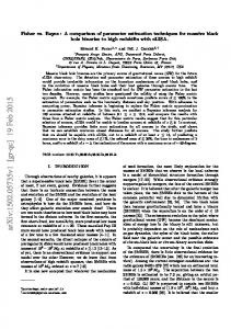
Figure 1: RMS error (-a-) and correlation coefficient (-b-) between true (measured) and estimated articulatory trajectories for ML and MAP (with various α values) learning, and corresponding filtered and smoothed estimation results.

∑ Nl − 1.

l=1

Therefore, the only unknown hyperparameter is {α }. The parameter α is estimated via trial and error. In this work, we test the values of α ∈ S = {0.1, 0.3, 0.5}.

for ML learning method while the corresponding results for MAP (α = 0.3) based learning method are about 1.93 mm and 0.59 respectively. That means MAP based learning algorithm in filtering mode reduces RMS error about 17.5% (from 2.34 mm to 1.93 mm) and improve the correlation coefficients about 13.4% (from 0.52 to 0.59). When we consider inferences based on smoothed estimate, The RMS error and correlation coefficient for ML based learning method are about 2.3 mm and 0.59, corresponding results for MAP (α = 0.3) based learning method are 1.85 mm and 0.65. That means MAP based learning algorithm in smoothing reduces RMS error about 18% (from 2.26 mm to 1.85 mm) and improve the correlation coefficients about 10% (from 0.59 to 0.65). The second observation from Fig.1 is that the smoothing is highly improves the performance compared to filtering. A similar result is reported in [3, 4] for articulatory inversion based on GMM and in [1] for articulatory inversion based on (TMDN). In our work smoothing reduces the RMSE from 2.34 mm to 2.26 mm (a 3.4% relative improvement) and improves the correlation coefficient about from 0.52 to 0.59 (a 13.4% relative improvement) when ML based learning is used. Similarly, smoothing reduces RMSE about 4.1% (from 1.93 mm to 1.85 mm) and improves correlation coefficient about 10.1% (from 0.59 to 0.65) for the MAP (α = 0.3) based learning method. Fig.2 provides more details regarding the utility of MAP based learning method in articulatory inversion. The abscissa distinguishes different articulators. As an example, in Fig.2, normalized RMS error for Y axis of upper lip (uly) reduced from 1.13 to 0.85. That means, there is a 24.7% relative error reduction. In general, this figure denotes that MAP based learning algorithm reduces normalized RMS about (14-28%). Fig.3 illustrates an example of the estimated (based on ML and MAP (α = 0.3) and the true x-coordinates of articulatory trajectories for lower incisor. The utterance is taken form MOCHA database.

4.3 Performance Measures The performance of the algorithms is measured using three performance measures, namely, RMS error, normalized RMS error and correlation coefficient, all of which are described in [1, 4, 10]. • RMS error: s 1 N i i ERMS , ∑ (xk − xˆki )2 , i = 1, . . . , m N k=1 where xki and xˆki are true and estimated position, respectively, of the ith articulator in the kth frame. • Normalized RMS error: i ERMS , σi

2.14

1.94

L

i ENRMS ,

Correlation Coefficient

l=1 k=2

v=

0.63

2.24

i = 1, . . . , m

where σi is the standard deviation of ith articulator xi . • Correlation coefficient: ∑Nk=1 (xki − x¯ki )(xˆki − x¯ˆki ) q ∑Nk=1 (xki − x¯ki )2 ∑Nk=1 (xˆki − x¯ˆki )2

ρx,i xˆ , q

for i = 1, . . . , m where x¯i and xˆ¯i are the average position of true and estimated ith articulator respectively. 4.4 Experimental Results Experimental results of the proposed method are given in this sub-section. The comparison of the learning methods based on ML and MAP criteria for a single GLDS in terms of RMS error and correlation coefficient can be seen in Fig.1. Examination of the figure shows that the MAP based learning method significantly improves the performance of the articulatory inversion. The performance of the proposed algorithm is tested for various α values and it is observed that α = 0.3 gives the best performance for MAP based learning algorithm. The RMS error and the correlation coefficient between the true (measured) and the estimated articulatory trajectories for filtering mode are about 2.34 mm and 0.52

5. CONCLUSION AND FUTURE WORK In this paper, we have examined parameter estimation methods that are based on ML and MAP criteria for acoustic-toarticulatory inversion which is done by using a single global linear dynamic system (GLDS). The main aim of this work

808

Normalized RMS Error

1.25

[2] C.Qin and M. Carreira-Perpin, “A comparison of acoustic features for articulatory inversion,” in Proc. INTERSPEECH, 2007. [3] T. Toda, A. W. Black, and K. Tokuda, “Statistical mapping between articulatory movements and acoustic spectrum using a Gaussian mixture model,” Speech Communication, vol. 50, pp. 215–227, 2008. ¨ [4] ˙I. Y. Ozbek, M. Hasegawa-Johnson, and M. Demirekler, “Formant trajectories for acoustic-to-articulatory inversion,” in Proc. INTERSPEECH, 2009. [5] S. Hiroya and M. Honda, “Estimation of articulatory movements from speech acoustics using an HMMbased speech production models,” IEEE Trans. Sp. Au. Proces, vol. 12, no. 2, p. 175185, March 2004. [6] A. Toutios and K. Margaritis, “Contribution to statistical acoustic-to-EMA mapping,” in EUSIPCO, 2008. ¨ H. Nam, X. Zhou, and C. Espy[7] V. Mitra, ˙I. Y. Ozbek, Wilson, “From acoustic to vocal tract time functions,” in ICASSP, 2009. [8] S. Ouni and Y. Laprie, “Modeling the articulatory space using a hypercube codebook for acoustic-toarticulatory inversion,” J. Acoust. Soc. Am., vol. 118, no. 1, pp. 444–460, 2005. [9] H. Kjellström and O. Engwall, “Audiovisual-toarticulatory inversion,” Speech Communication, vol. 51, no. 3, pp. 195–209, 2009. [10] A. Katsamanis, G. Papandreou, and P. Maragos, “Face active appearance modeling and speech acoustic information to recover articulation,” IEEE Trans. Acoust., Speech, Signal Process., vol. 17, no. 3, pp. 411–422, 2009. [11] A. Katsamanis, G. Ananthakrishnan, G. Papandreou, P. Maragos, and O. Engwall, “Audiovisual speech inversion by switching dynamical modeling governed by a hidden markov process,” in Proc. EUSIPCO, 2008. [12] S. Dusan and L. Deng, “Acoustic-to-articulatory inversion using dynamical and phonological constraints,” in 5’th Seminar on Speech Production: Models and Data, Kloster Seeon,Germany, 2000, pp. 237–240. [13] L. J. Lee, P. Fieguth, and L. Deng, “A functional articulatory dynamic model for speech production,” in Proc. ICASSP, 2001, pp. 797–800. [14] R. Tibshirani, “Regression shrinkage and selection via the lasso,” J. Royal. Statist. Soc B., vol. 58, no. 1, pp. 267–288, 1996. [15] T. P. Minka, “Bayesian linear regression,” 3594 Security Ticket Control, Tech. Rep., 1999. [16] D. B. Rowe, Multivariate Bayesian Statistics: Models for Source Separation and Signal Unmixing. New York: CRC Press Company, 2003. [17] D. Simon, Optimal State Estimation: Kalman, H∞ , and Nonlinear Approaches. Wiley, 2006. [18] A. Wrench and W. Hardcastle, “A multichannel articulatory speech database and its application for automatic speech recognition,” in In Proc. 5th Seminar on Speech Production, 2000, [Online]. Available: http://www.cstr.ed.ac.uk/artic.

ML Learning MAP Learning

1.15 1.05 0.95 0.85 0.75 0.65

lix

liy

ulx

uly

llx

lly

ttx tty Articulators

tbx

tby

tdx

tdy

vx

vy

Lower Incisor X−Axis Position (mm)

Figure 2: Normalized RMS errors for each articulator for ML and MAP (α = 0.3) learning methods. The abbreviations li, ul,ll, tt,tb, td and v denote lower incisor, upper lip, lower lip, tongue tip, tongue body, tongue dorsum and velum, respectively. The suffixes x and y of the articulator abbreviations show the corresponding X and Y coordinates respectively.

1 0 −1 True ML MAP (α=0.3)

−2 −3

0

0.5

1 Time (sec)

1.5

2

Figure 3: An example of estimated (based on ML and MAP method) and true articulatory trajectories of x-coordinate for lower incisor.(taken from MOCHA database) is to show that MAP based parameter estimation method significantly improves the performance of the articulatory inversion. Experiments have been conducted on the MOCHA databases. In the literature, [11] uses a single GLDS in articulatory inversion with similar experimental setup. They estimate the model parameter set via ML criterion and their best RMSE and correlation coefficient results between the true (measured) and estimated articulatory trajectories are 2.15 mm and 0.59 respectively. According to the experimental results given in Sec. 4.4, our best results are obtained via MAP based learning algorithm by using smoothing method. The RMS error and correlation coefficient are about 1.85 mm and 0.65 respectively, which is significantly better than the results of [11]. The main reason of the improvement is using MAP based learning instead of ML and also smoothing instead of filtering. Our future work plan is to generalize the single GLDS to a multiple models dynamic system which is known as jump Markov linear system (JMLS) or switching linear dynamic system (SLDS) and use MAP based learning. The preliminary experimental results showed that MAP based learning algorithm is also improves the performance of articulatory inversion when multiple models are used. REFERENCES [1] K. Richmond, “Estimating articulatory parameters from the speech signal,” Ph.D. dissertation, The Center for Speech Technology Research, Edinburgh, KU, 2002.

809