Aug 12, 2015 - ... (Emeritus), The Graduate School and University Center (CUNY) .... sequences of formulas, which we cal
Modal Interpolation via Nested Sequents Melvin Fittinga,1 , Roman Kuznetsb,c,2,3,∗ a Department
of Computer Science (Emeritus), The Graduate School and University Center (CUNY) b Institut f¨ ur Informatik und angewandte Mathematik, Universit¨ at Bern c Institut f¨ ur Computersprachen, Technische Universit¨ at Wien
Abstract The main method of proving the Craig Interpolation Property (CIP) constructively uses cut-free sequent proof systems. Until now, however, no such method has been known for proving the CIP using more general sequent-like proof formalisms, such as hypersequents, nested sequents, and labelled sequents. In this paper, we start closing this gap by presenting an algorithm for proving the CIP for modal logics by induction on a nested-sequent derivation. This algorithm is applied to all the logics of the so-called modal cube. Keywords: Craig interpolation, nested sequent, structural proof theory, modal logic 2010 MSC: 03B45, 03C40, 03F07
1. Introduction Suppose, for the moment, that we identify a logic with a set of formulas L, ignoring semantics, proof systems, and so on. Then L has the Craig interpolation property (CIP) if, whenever A ⊃ B ∈ L, there exists a formula C such that A ⊃ C, C ⊃ B ∈ L, where C is in the “common language” of A and B. What “common language” means is situation-dependent: it can mean having shared propositional variables, or individual variables, or modal operators, or nominals, etc. Whether a logic has the CIP is an important characteristic of the logic (for an overview of the problems and complexity of interpolation, as well as a history of the subject, see [6]). In addition to knowing whether a logic has the CIP, it is useful to be able to prove the property constructively.4 For instance, in [12], the existence of fixed points in the logic of provability GL was established constructively using the CIP of GL, and in [3], that method was made the basis of a program to compute fixed points for GL. Historically, constructive proofs of the CIP for L make use of a cut-free proof system for L, typically a sequent calculus or tableau system. Unfortunately, sequent calculi for modal logics whose semantics involves symmetry are hard to come by, though sometimes ad hoc methods have been devised. Actually, cut-freeness is not the central issue. What is important is that we have a proof procedure that has the subformula property and in which polarity of subformulas is preserved during the course of a proof. (Both are violated by the cut rule.) Over the years generalizations of sequent and tableau systems have been developed, capable of handling a greater number of logics in a uniform way: among them, nested sequents ([1]) ∗ Corresponding
author collaboration was made possible by several visits of this author to Bern, thanks to the financial support of the Swiss National Science Foundation Grants 200020-134740 and PZ00P2-131706. 2 In 2011–2013, this author was supported by the Swiss National Science Foundation Grant PZ00P2-131706. The final stages of the research were supported by the Austrian Science Fund Grants Y 544 and P 25417. 3 Affiliation b of this author corresponds to the period up until February 2014, when most of the work on this paper was done. Affiliation c of this author is his current affiliation and corresponds to the preparation of the final version of the paper. 4 As pointed out to us by Matthias Baaz, for a recursively enumerable logic, any proof of the CIP yields a (very inefficient) algorithm for constructing an interpolant by enumerating all theorems until an interpolant is found. The obvious disadvantage of such an algorithm is in the difficulty of giving any, however weak, estimates of its efficiency. Our method provides a more reasonable construction based on a nested-sequent derivation with complexity bounded by the size of the derivation. It should be mentioned that the resulting complexity is not polynomial in the size of the derivation and, hence, not optimal. 1 This
Preprint submitted to Elsevier
August 12, 2015
and prefixed tableaus ([2, 11]). Nested sequents are in the tradition allowing so-called deep reasoning in the course of a proof. Prefixed tableaus allow a kind of representation of possible worlds directly in the proof, with accessibility captured using simple syntactic machinery. It turns out that nested sequents and prefixed tableaus are related much as ordinary sequents and tableaus are—loosely, one is the other upside-down ([4]). In this paper, we show that nested sequents can be used in a natural way to prove the CIP constructively for all the logics in the modal cube. There is no appeal to ad hoc methods; the work is essentially uniform across the whole family. While our primary interest is in interpolants between two formulas or, more generally, two sets of formulas, we develop something broader: we introduce the notion of interpolant between sets of formulas within a nested structure. Interpolants created at this level cannot be just formulas. Instead, our interpolants are Boolean combinations of formulas within the same nested structure. Thus, we actually work with a more general notion of interpolant. Interpolation in the usual sense is a special case. We assume we have a countable set Prop of propositional variables, fixed throughout this paper. Our modal language L is built up from these propositional variables, together with > and ⊥, in the usual way, using propositional connectives ¬, ∧, ∨, and ⊃ and modal operators � and ♦. We omit parentheses when it will not lead to confusion. For a modal formula A, by Prop(A) we mean the set of propositional variables that occur in A. We note that all logics considered here are monomodal, though proof systems of the sort we use do exist for multimodal logics as well. Definition 1.1 (CIP for modal logics). A modal logic L has the CIP if for any formulas A and B such that A ⊃ B ∈ L, there exists an interpolant C such that A ⊃ C ∈ L,
C ⊃ B ∈ L,
and
Prop(C) ⊆ Prop(A) ∩ Prop(B) .
Thus, common language for modal logics simply means having common propositional variables. Unlike with ordinary sequent calculi, there are cut-free nested sequent systems for each normal modal logic formed from any combination of axioms d, t, b, 4, and 5. The difficulty in extracting interpolants from nested sequent proofs lies in the presence in nested sequents of an additional structural connective that corresponds to � the same way that comma in ordinary sequents corresponds to ∧ in the antecedent or to ∨ in the consequent of a two-sided sequent. This additional nested structure has to be reflected in the interpolation process, and this is the source of most of the technical complexity to be found here. 2. Nested Sequent Calculus for the Basic Normal Monomodal Logic K Definition 2.1 (Logic K). The minimal normal monomodal logic K is the logic of all Kripke frames. It is axiomatized by • an arbitrary complete set of axioms of classical propositional logic (in the monomodal language L), • the rule modus ponens, • the normality axiom k: �(A ⊃ B) ⊃ (�A ⊃ �B), • the necessitation rule:
A . �A
We identify the logic K with the set of its theorems and write K ` A instead of A ∈ K. Before presenting a nested sequent calculus for K, we need to define nested sequents, the objects of the derivation in such a calculus, and contexts, the tools necessary to describe rules of such a calculus. We define a grammar for nested objects that covers both sequents and contexts and explain how to distinguish between them. Definition 2.2 (Nested objects). We define nested objects Φ according to the following grammar: Φ ::= ε | Φ, A | Φ, { } | Φ, [Φ] 2
,
where ε is the empty sequence, A ∈ L is a formula, { } is the hole symbol, brackets in [Φ] are called a structural box, and comma is the operation of appending an element to the end of a sequence. Thus, a nested object is a sequence of formulas, of occurrences of the hole symbol, and of nested objects within structural boxes. It is trivial to define the number of occurrences of the hole symbol in a given nested object, which is why we omit the formal definition. Definition 2.3 (Nested sequents, contexts, and multicontexts). A nested object without holes is called a nested sequent, or, simply, a sequent. A nested object with exactly one hole is called a context. A nested object with more than one hole is called a multicontext. In this paper, we do not use multicontexts, although they do play a significant role elsewhere. Thus, from now on, all nested objects are assumed to be either sequents or contexts. Since there is exactly one hole in a context, we call it the hole. We use Γ, ∆, . . . , possibly with sub- and/or superscripts, to denote sequents, Γ{ }, ∆{ }, . . . , possibly with sub- and/or superscripts, to denote contexts, and Φ, Ψ, . . . , possibly with sub- and/or superscripts, to denote nested objects that can be either sequents or contexts. One way of looking at a nested sequent is to consider a tree of ordinary one-sided sequents, i.e., of sequences of formulas, which we call here shallow sequents to avoid ambiguity. Each structural box in the nested sequent corresponds to a child in the tree. Nested sequent calculi are designed to use the mechanism of deep inference, where rules are applied at an arbitrary node of this tree, i.e., arbitrarily deep in the nested structure of the sequent. The hole in a context provides a reference to the place, or to the node in the tree, at which the rule should be applied. Definition 2.4 (Inserting a sequent into a nested object). The insertion of a sequent ∆ into a nested object Φ is obtained by performing the following action on Φ: if Φ contains the hole, replace it with ∆; otherwise, do not do anything. The result of such an insertion is denoted Φ{∆}. When we use the notation Φ{∆{Γ}}, it should be read as follows: first, the sequent Γ is inserted into the context ∆{ }; second, the resulting sequent ∆{Γ} is inserted into the nested object Φ. Figure 1 recalls the uniform notation, which is typical of tableau calculi and which we use in the paper. α A∧ B ¬(A∨B) ¬(A ⊃ B)
α1 A ¬A A
ν �A ¬♦A
α2 B ¬B ¬B
β A∨ B ¬(A∧B) A⊃B
ν0 A ¬A
π ♦A ¬�A
β1 A ¬A ¬A
β2 B ¬B B
π0 A ¬A
Figure 1: Uniform notation.
Definition 2.5 (Nested sequent calculus NK). The nested sequent calculus NK for the modal logic K can be found in Figure 2. This calculus is a hybrid of the multiset-based version from [1], where formulas are restricted to the negation normal form, of the sequence-based version from [8], where formulas are also restricted to the negation normal form, and of the set-based version from [4], where formulas are unrestricted. None of the three versions uses Boolean constants ⊥ and >, necessitating an addition of the rules id> and id¬⊥ for handling these. According to the uniform notation, the α and β rules in Figure 2 encode three rules each and the ν and π rules encode two rules each. In [1, 8], the ν and π rules are called the � and k rules respectively. 3
−−−−−−−−− − idP − Γ{P, ¬P }
Γ{A}
¬¬
− −−−−−−−− − Γ{¬ ¬ A}
Γ{A, A}
−−−−−−− − ctr −
Γ{A}
id> −−−−−−
Γ{>}
Γ{β1 , β2 } −−−−−−−−− − β− Γ{β}
Γ{∆, Σ}
−−−−−− − id¬⊥ − Γ{¬⊥}
Γ{α1 } Γ{α2 } −−−−−−−−−−−−−−− − α− Γ{α}
Γ{[ν0 ]} −−−−−− − ν−
exch −−−−−−−−−
Γ{Σ, ∆}
Γ{ν}
Γ{[∆, π0 ]} −−−−−−−−−− − π− Γ{[∆], π}
Figure 2: Rules of the nested sequent calculus NK.
� Example 2.6. A nested sequent derivation of �(P ⊃ �Q) ⊃ �(�Q ⊃ R) ⊃ �(P ⊃ R) can be found in Figure 3.
− −−−−−−−−−−−−−−−− − idP � � ¬P, R, [Q, ¬Q] − −−−−−−−−−−−−−−−−−− − π� � ¬P, R, [Q], ¬�Q − − − − − − − − − − − − − − − − − − − − exch � � (††) idP −−−−−−−−−−−−−−−−−−− ¬P, R, ¬�Q, [Q] [¬P, R, ¬R, ¬�Q] −−−−−−−−−−−−−−−−−−−−−−−− − −−−−−−−−−−−−−−−−−− − (?) −−−−−−−−−−−−−−−−− − idP − ν− exch − [P, ¬P, R, ¬(�Q ⊃ R)] [¬P, R, ¬�Q, �Q] [¬P, R, ¬�Q, ¬R] −−−−−−−−−−−−−−−−−−−−−−−− − (†) −−−−−−−−−−−−−−−−−−−−−−−−−−−−−−−−−−−−−−−−−−−−−−−−−−− − exch − α− [¬P, R, P, ¬(�Q ⊃ R)] [¬P, R, ¬�Q, ¬(�Q ⊃ R)] −−−−−−−−−−−−−−−−−−−−−−−−−−−−−−−−−−−−−−−−−−−−−−−−−−−−−−−−−−−−−−−−−−−−−−−−−−−−− − α− [¬P, R, ¬(P ⊃ �Q), ¬(�Q ⊃ R)] −−−−−−−−−−−−−−−−−−−−−−−−−−−−−−−−−−−−− − β− [P ⊃ R, ¬(P ⊃ �Q), ¬(�Q ⊃ R)] −−−−−−−−−−−−−−−−−−−−−−−−−−−−−−−−−−−−−−− − π− [P ⊃ R, ¬(P ⊃ �Q)], ¬�(�Q ⊃ R) −−−−−−−−−−−−−−−−−−−−−−−−−−−−−−−−−−−−−−− − exch − ¬�(�Q ⊃ R), [P ⊃ R, ¬(P ⊃ �Q)] −−−−−−−−−−−−−−−−−−−−−−−−−−−−−−−−−−−−−−−−− − π− ¬�(�Q ⊃ R), [P ⊃ R], ¬�(P ⊃ �Q) −−−−−−−−−−−−−−−−−−−−−−−−−−−−−−−−−−−−−−−−− − (††††) exch − ¬�(P ⊃ �Q), ¬�(�Q ⊃ R), [P ⊃ R] −−−−−−−−−−−−−−−−−−−−−−−−−−−−−−−−−−−−−−−−−−−− − (??) ν− ¬�(P ⊃ �Q), ¬�(�Q ⊃ R), �(P ⊃ R) −−−−−−−−−−−−−−−−−−−−−−−−−−−−−−−−−−−−−−−−−−−−− − β− ¬�(P ⊃ �Q), �(�Q ⊃ R) ⊃ �(P ⊃ R) −−−−−−−−−−−−−−−−−−−−−−−−−−−−−−−−−−−−−−−−−−−−−−−− − β− �
(†††)
�(P ⊃ �Q) ⊃ �(�Q ⊃ R) ⊃ �(P ⊃ R)
� Figure 3: An NK derivation of �(P ⊃ �Q) ⊃ �(�Q ⊃ R) ⊃ �(P ⊃ R) .
To understand in which sense this nested calculus represents the modal logic, we need a translation from sequents to formulas of this modal logic. Intuitively, our sequents are one-sided (i.e., comprising only the consequent part of a two-sided sequent) with two structural connectives: structural disjunction (comma ,) and structural necessitation modality (bracket [·]). This intuition is formalized using the notion of a corresponding formula. Since this notion does not make sense for contexts, we use the following subgrammar that defines sequents: Γ ::= ε | Γ, A | Γ, [Γ] . This subgrammar will also be used in proofs by induction on the structure of a given sequent. Definition 2.7 (Corresponding formula of a nested sequent). For any sequent Γ, its corresponding
4
formula Γ is defined by induction on the construction of the sequent: ( ( Γ∨A if Γ 6= ε, Γ∨�∆ Γ, A := Γ, [∆] := ε := ⊥; A otherwise; �∆
if Γ 6= ε, otherwise.
The following theorem follows from the results in [1, 4, 8]. Theorem 2.8 (Completeness of the calculus NK). For any sequent Γ, we have NK ` Γ iff K ` Γ iff Γ, where expresses validity in the class of all Kripke models. 3. Formulating Interpolation for Nested Sequents Our goal is to prove the CIP by induction on the nested sequent derivation. To achieve this, it is necessary to decide what being an interpolant of a nested sequent means and what kind of object an interpolant of a nested sequent is. Since the answers to these questions have turned out to be quite non-trivial, we first explain how we arrived at these answers by using an analogy with the formalism closest to nested sequents: namely, shallow one-sided sequents, i.e., multisets of formulas. We show why for nested sequents it is not possible to directly use the definitions of interpolation and interpolant known from shallow sequents and explain in which sense our definitions conform to the idea of interpolation and how they are formally related to the CIP, whose formulation is independent of the proof system used. Definition 3.1 (Interpolant of a shallow one-sided sequent). Let a multiset of formulas ∆ be partitioned into two multisets L (∆) and R (∆). Whenever safe, we omit the parentheses. We call L∆ | R∆ a split of ∆. An interpolant of the split L∆ | R∆ of the sequent ∆ is a formula C such that ¬C
L∆,
C R∆ ,
and C only uses propositional variables common to L∆ and R∆. For a given shallow one-sided sequent calculus, this statement is usually formulated syntactically in terms of derivability in the calculus; however, as we explain later, interpolants of nested sequents cannot be restricted to the formula format. Since an introduction of yet another calculus just for the purpose of formulating the interpolation statement syntactically does not seem reasonable, our interpolation statements for nested sequents are formulated semantically, and the statement above is the closest analog. Example 3.2. Before giving formal definitions, let us consider a simple example to motivate our choices. A shallow sequent Q, R, P, ¬P is derivable by idP . One of the possible splits is Q, R, ¬P | P , and the interpolant prescribed to such a split by most sequent-based is P . � � � algorithms � ¬P , derivable by the same rule idP . It should be possible Let us now consider the sequent ∆ �= Q,� R� , P, � � � to split this sequent in the same way: Q, R , ¬P | P . However, the information that P and ¬P are in the same structural box, which makes the sequent derivable, is lost in such a split. Thus, instead of creating the split by physically moving formulas in the sequent, we indicate to which side of the split each formula should belong by assigning it a bias � in the � � form of �a superscript. The above-mentioned split is then represented by e = Q` , R` , P < , ¬P ` . The left (right) side of such a biased sequent is obtained by the biased sequent ∆ dropping all right-biased (left-biased) formulas and erasing the biases of the remaining formulas: e = [Q, R], [¬P ] , L∆
e = [ε], [P ] . R∆
Note that the structural boxes are not removed even if they become empty. � � Let us simplify further. Suppose we want to find an interpolant of P, ¬P biased in the � − e `
Γ{> }
l ¬¬
e `} Γ{A
− −−−−−−−−− − e ¬ ¬ A` } Γ{
e ` } Γ{α e `} Γ{α 1 2 −−−−−−−−−−−−−−− − αl − e ` Γ{α }
e − e
}
r ¬¬
Γ{ ⊥ }
e }
e < } ←− f1 Γ{α e < } ←− f2 Γ{α 1 2 −−−−−−−−−−−−−−−−−−−−−−−−−−−−−−−−−−−− − αr − e < } ←− f1 7 f2 Γ{α
e ` } ←− f1 Γ{α e ` } ←− f2 Γ{α 1 2 −−−−−−−−−−−−−−−−−−−−−−−−−−−−−−−−−−− − αl − e ` } ←− f1 6 f2 Γ{α n
e ∆], e [Σ]} e ←− Γ{[
mi
6 Λij {[∆ij ], Aij , [Σij ]} 7 i=1 j=1
−−−−−−−−−−−−−−−−−−−−−−−−−−−−−−−−−−−−−−−−−−−−−−−−−− − adtr[ ][ ] − n mi
e Σ], e [∆]} e ←− Γ{[
n
e ` ]} Γ{[ν 0
←−
l
6 Λij {[Σij ], Aij , [∆ij ]} 7 i=1 j=1 mi
li
!
7 Λij {[ε]} 6 7 Πik {[Aik ]} 7 j=1 i=1 k=1
−−−−−−−−−−−−−−−−−−−−−−−−−−� −−−−−−−−−−− −−−−−−−−−−−−−−−−−−− − ν − ! � mi n li V e ◦ {♦ e ` } ←− Γ Aik } 7 Γ{ν Λij {ε} i=1 j=1 k=1
6
n
e < ]} ←− Γ{[ν 0 r
7
li
mi
!
7 6 Πik {[Aik ]} 6 j=1 6 Λij {[ε]} i=1 k=1
−−−−−−−−−−−−−−−−−−−−−−−−−−−� −−−−−−−−−−− −−−−−−−−−−−−−−−−−−− − ν − ! � mi n li W < ◦ e e Γ{ν } ←− Γ {� Aik } 6 Λij {ε} i=1 j=1 k=1
7
6
For all the remaining rules, i.e., for the rules ¬¬l , ¬¬r , ctrl , ctrr , β l , β r , adtrlrff , adtrrlff , adtrllff , adtrrr ff , adtrlf[ ] , adtrrf[ ] , adtrl[ ]f , adtrr[ ]f , π l , and π r , the given interpolant for the premise is used as an interpolant for the conclusion. Figure 6: Interpolation algorithm for the calculus BNK. Interpolants for the premises of adtr[ ][ ] and ν r must be in a SCNF; e } ∼ Λij { } ∼ Πik { } for all an interpolant for the premise of ν l must be in a SDNF. For these three rules, we require that Γ{ suitable i, j, and k. Finally, Aij in adtr[ ][ ] must be shallow sequents for all suitable i and j.
18
Example 6.2. Let us apply the algorithm to the derivation of ¬�(P ⊃ �Q)` , �(�Q ⊃ R) ⊃ �(P ⊃ R)< from Figure 5. The result can be found in Figure 7. Since most of the rules do not require the interpolant to be changed, we only explain those steps of the algorithm that do, starting from the three leaves of e 1 {P ` , ¬P < } the derivation tree. The leftmost leaf, an application of the rule idlrP , has the conclusion Γ < ¬ < ◦ e e with Γ1 = [{ }, R , (�Q ⊃ R) ]. Given that Γ1 = [{ }], we assign to this conclusion an interpolant e ◦ {¬P } = [¬P ]. Similarly, the middle leaf, an application of the rule idrl with the conclusion Γ e {Q< , ¬Q` } Γ 1 � < < � � �P � � 2 ◦ ◦ e e e where Γ2 = ¬P , R , [{ }] , is assigned an interpolant Γ2 {Q} = [Q] , where Γ2 = [{ }] . Finally, the < ¬ < ` e e ¬ < ¬ rightmost leaf, an application of the rule idrr P with the conclusion Γ3 {R , R } where Γ3 = [ P , { }, �Q ], e ◦ {>} = [>], where Γ e ◦ = [{ }]. is assigned an interpolant Γ 3 3 There are two α rules in the derivation. The first, αr , requires taking the external conjunction of [�Q] and [>]. The second rule, αl , produces the external disjunction of [¬P ] with the external conjunction [�Q] 7 [>]. In both cases, the result is clearly well formed. In Lemma 6.4(ii), we show that external conjunctions and disjunctions are always applicable to interpolants in the premises of α rules. It remains to explain how the ν rules are applied (both are ν r rules). First, in (?), from the inter� � � � e 4 {[Q< ]} = ¬P < , R< , ¬�Q` , [Q< ] with Γ e 4 { } = [¬P < , R< , ¬�Q` , { }], we construct an interpolant [Q] of Γ � � e 4 {�Q< } = [¬P < , R< , ¬�Q` , �Q< ]. The interpolant of the premise [Q] is in the prescribed SCNF polant of Γ < ¬ ` e ¬ < with its only disjunct of its only conjunct being Π{[Q]} for W Π{ } = [{ }] ∼ [ P , R , �Q , { }] = Γ4 { }. To compute the interpolant [�Q] of the conclusion, we take {Q} = Q, prefix it with a �, and insert �Q into e ◦ { } = [{ }]. Γ 4 � Finally, we discuss (??). The preceding rule adtrlrff yields the interpolant [¬P ]6 [�Q]7[>] of the premise e 5 {[P ⊃ R< ]} = ¬�(P ⊃ �Q)` , ¬�(�Q ⊃ R)< , [P ⊃ R< ] with Γ e 5 { } = ¬�(P ⊃ �Q)` , ¬�(�Q ⊃ R)< , { }. Γ < e 5 {�(P ⊃ R) } = ¬�(P ⊃ �Q)` , ¬�(�Q ⊃ R)< , �(P ⊃ R)< , To construct an interpolant of the conclusion Γ � we first need to convert [¬P ] 6 [�Q] 7 [>]� to a SCNF using the constructive method from Fact � � � 5.7. � � The result, [¬P ] 6 [�Q] 7 [¬P ] 6 [>] = Π1,1 {[¬P ]} 6 Π1,2 {[�Q]} 7 Π2,1 {[¬P ]} 6 Π2,2 {[>]} with e 5 {}, is also an interpolant of the premise by Lemma 5.8. Since Π1,1 {} = Π1,2 {} = Π2,1 {} = Π2,2 {} = {} ∼ Γ ◦ e e ◦ {�(¬P ∨�Q)} 7 Γ e ◦ {�(¬P ∨>)} = �(¬P ∨�Q) 7 �(¬P ∨>). Γ = { }, the interpolant of the conclusion is Γ 5
5
idlr P adtrrl ff adtrrl ff αl
Converting
5
− −−−−−−−−−−−−−−−−−−−−−−−− idrl �−−−−−−−�−−−−−� P � ¬P < , R< , [Q< , ¬Q` ] ←− [Q] − −−−−−−−−−−−−−−−−−−−−−−−−−− πl � �−−−−−−−�−−−−−� ¬P < , R< , [Q< ], ¬�Q` ←− [Q] −−−−−−−−−−−−−−−−−−−−−−−−−− −−−−−−− −−−−−−−−−−−−−−−−−−−−−−−−−−−−−−−−−− − − −−−−−−−−−−−−−−−−−−−−−−−−−−−−−−−−−−−−−−−−−− − adtrlf[ ] − idrr � � �−−−−−� (††) P − ¬P < , R< , ¬�Q` , [Q< ] ←− [Q] [P ` , ¬P < , R< , ¬(�Q ⊃ R)< ] ←− [¬P ] [¬P < , R< , ¬R< , ¬�Q` ] ←− [>] −−−−−−−−−−−−−−−−−−−−−−−−−−−−−−−−−−−−− − (?) − − − − − − − − − − − − − − − − − − − − − − − − − − − − − − − − − − − − − −−−−−−−−−−−−−−−−−−−−−−−−−−−−−−−−−−−−−−−−−− − (†) νr − adtrlr ff [¬P < , P ` , R< , ¬(�Q ⊃ R)< ] ←− [¬P ] [¬P < , R< , ¬�Q` , �Q< ] ←− [�Q] [¬P < , R< , ¬�Q` , ¬R< ] ←− [>] −−−−−−−−−−−−−−−−−−−−−−−−−−−−−−−−−−−−−−−−−−−−−−−−−−−−−−−−−−−−−−−−−−−−−−−−−−−−−−−−−−−−−−− − − −−−−−−−−−−−−−−−−−−−−−−−−−−−−−−−−−−−−−−−−−− − (†) αr − < < ` < < < ` < [¬P , R , P , ¬(�Q ⊃ R) ] ←− [¬P ] [¬P , R , ¬�Q , ¬(�Q ⊃ R) ] ←− [�Q] 7 [>] − −−−−−−−−−−−−−−−−−−−−−−−−−−−−−−−−−−−−−−−−−−−−−−−−−−−−−−−−−−−−−−−−−−−−−−−−−−−−−−−−−−−−−−−−−−−−−−−−−−−−− −−−−−−−−−−−−−−−−−−−−−−−−−−− − � [¬P < , R< , ¬(P ⊃ �Q)` , ¬(�Q ⊃ R)< ] ←− [¬P ] 6 [�Q] 7 [>] −−−−−−−−−−−−−−−−−−−−−−−−−−−−−−−−−−−−−−−−−−−−−−−−−−−−−−−−−−−−−−−−−−−−−−− − βr − � [P ⊃ R< , ¬(P ⊃ �Q)` , ¬(�Q ⊃ R)< ] ←− [¬P ] 6 [�Q] 7 [>] −−−−−−−−−−−−−−−−−−−−−−−−−−−−−−−−−−−−−−−−−−−−−−−−−−−−−−−−−−−−−−−−−−−−−−−− − πr − � [P ⊃ R< , ¬(P ⊃ �Q)` ], ¬�(�Q ⊃ R)< ←− [¬P ] 6 [�Q] 7 [>] −−−−−−−−−−−−−−−−−−−−−−−−−−−−−−−−−−−−−−−−−−−−−−−−−−−−−−−−−−−−−−−−−−−−−−−− − adtrrf[ ] − � ¬�(�Q ⊃ R)< , [P ⊃ R< , ¬(P ⊃ �Q)` ] ←− [¬P ] 6 [�Q] 7 [>] −−−−−−−−−−−−−−−−−−−−−−−−−−−−−−−−−−−−−−−−−−−−−−−−−−−−−−−−−−−−−−−−−−−−−−−−−− − πl − � ¬�(�Q ⊃ R)< , [P ⊃ R< ], ¬�(P ⊃ �Q)` ←− [¬P ] 6 [�Q] 7 [>] −−−−−−−−−−−−−−−−−−−−−−−−−−−−−−−−−−−−−−−−−−−−−−−−−−−−−−−−−−−−−−−−−−−−−−−−−− − adtrlf[ ] − � (††††) ¬�(�Q ⊃ R)< , ¬�(P ⊃ �Q)` , [P ⊃ R< ] ←− [¬P ] 6 [�Q] 7 [>] − − − − − − − − − − − − − − − − − − − − − − − − − − − − − − − − − − − − − − − − − − − − − − − − − − − − − − − − − − − − − − − − − − − − − − − − − − − − adtrlr � (††††) ff ¬�(P ⊃ �Q)` , ¬�(�Q ⊃ R)< , [P ⊃ R< ] ←− [¬P ] 6 [�Q] 7 [>] −−−−−−−−−−−−−−−−−−−−−−−−−−−−−−−−−−−−−−−−−−−−−−−−−−−−−−−−−−−−−−−−−−−− −−−−−−−−−−−−−−−−− − interpolant to SCNF − � � ¬�(P ⊃ �Q)` , ¬�(�Q ⊃ R)< , [P ⊃ R< ] ←− [¬P ] 6 [�Q] 7 [¬P ] 6 [>] −−−−−−−−−−−−−−−−−−−−−−−−−−−−−−−−−−−−−−−−−−−−−−−−−−−−−−−−−−−−−−−−−−−−−−−−−−−−−−−−−−−−− − (??) νr − ¬�(P ⊃ �Q)` , ¬�(�Q ⊃ R)< , �(P ⊃ R)< ←− �(¬P ∨�Q) 7 �(¬P ∨>) −−−−−−−−−−−−−−−−−−−−−−−−−−−−−−−−−−−−−−−−−−−−−−−−−−−−−−−−−−−−−−−−−−−−−−−−−−−−−−−−− − βr − ¬�(P ⊃ �Q)` , �(�Q ⊃ R) ⊃ �(P ⊃ R)< ←− �(¬P ∨�Q) 7 �(¬P ∨>)
Figure 7: Application of Algorithm 6.1 to the BNK-derivation of ¬�(P ⊃ �Q)` , �(�Q ⊃ R) ⊃ �(P ⊃ R)< from Figure 5.
Let us now prove that the interpolation algorithm works for all biased derivations. We start with the 19
(†††)
simplest of the three lemmas that states that the propositional variables of the interpolant produced by the algorithm are always common to the left and right sides of the biased sequent being interpolated. Lemma 6.3. For every rule in Figure 6, if the propositional variables of the given interpolant in each premise are common to the left and right sides of the biased sequent in this premise, then the propositional variables of the newly constructed interpolant for the conclusion are common to the left and right sides of the biased sequent in the conclusion. Proof. We leave this as an exercise to be checked by the reader with the help of the fact that � � � � e Π}) e e }) ∪ Prop(LΠ) e e Π}) e e }) ∪ Prop(RΠ) e . Prop L(Γ{ = Prop(LΓ{ and Prop R(Γ{ = Prop(RΓ{ In the second lemma, we demonstrate all the necessary properties of the structure of interpolants: Lemma 6.4. (i) To apply the algorithm to the rule adtr[ ][ ] , rule ν l , or rule ν r , a given interpolant for the premise of the rule must be in the required form (see Figure 6). If the given interpolant is not in this form, it can be efficiently converted to a decoratively equivalent generalized sequent that is. (ii) The object suggested by the algorithm as an interpolant for the conclusion of all zero-premise rules, as well as for the rule αl , rule αr , rule adtr[ ][ ] , rule ν l , and rule ν r , is always a well-formed generalized sequent (provided, for the rule adtr[ ][ ] , rule ν l , and rule ν r , that a given interpolant for the premise of the rule is in the required form).7 (iii) Each generalized sequent suggested by the algorithm for the conclusion of any rule is structurally equivalent to the biased sequent from this conclusion. Proof. For each rule, we need to prove all statements applicable to it. For brevity, we say “interpolant” instead of “suggested interpolant.” l r l r 8 (ii) and (iii) for idlrP , idrlP , idllP , idrr P , id> , id> , id¬⊥ , and id¬⊥ . The details are left to the reader. r l r l l r (iii) for ¬¬l , ¬¬r , ctrl , ctrr , β l , β r , adtrlrff , adtrrlff , adtrllff , adtrrr ff , adtrf[ ] , adtrf[ ] , adtr[ ]f , adtr[ ]f , π , and π . For e Π} e each rule, given that the interpolant remains unchanged, to show the structural equivalence of a premise Γ{ e Λ} e of each rule, it is sufficient to show that Π e ∼ Λ. e The details are left to the reader. and a conclusion Γ{ l r l ` ` ` e e e (ii) and (iii) for α and α . For α , since Γ{α 1 } ∼ Γ{α2 } ∼ Γ{α }, it follows that f1 ∼ f2 . Thus, f1 6 f2 e ` } ∼ Γ{α e ` }. The case of αr is analogous. is defined. Further, f1 6 f2 ∼ f1 ∼ Γ{α 1
e ∆], e [Σ]} e (i), (ii), and (iii) for adtr[ ][ ] . Let us start with transforming a given interpolant f for a premise Γ{[ 0 e e e into the required form. By Fact 5.7 and Lemma 5.8, another interpolant f of Γ{[∆], [Σ]} can be constructed that is in a SCNF. Further, every member sequent Ω of the interpolant f0 is structurally equive ∆], e [Σ]}, e e ◦ {[∆ e ◦ ], [Σ e ◦ ]}. Thus, by Lemma 5.9.2, Ω = Λ{[Π], A, [Θ]} where alent to Γ{[ meaning that Ω◦ = Γ ◦ ◦ ◦ ◦ ◦ ◦ e { }, Π = ∆ e , Θ = Σ e , and A is a shallow sequent9 . It follows that Λ{ } ∼ Γ{ e }, which Λ {} = Γ completes the proof of (i). Each member sequent Λij {[Σij ], Aij , [∆ij ]} of the interpolant for the cone ∆], e [Σ]}, e clusion corresponds to the member sequent Λij {[∆ij ], Aij , [Σij ]} of the given interpolant of Γ{[ e e e e where Λij { } ∼ Γ{ }. Since Λij {[∆ij ], Aij , [Σij ]} ∼ Γ{[∆], [Σ]} by assumption, [∆ij ], Aij , [Σij ] must be e [Σ], e meaning that ∆ij ∼ ∆ e and Σij ∼ Σ. e It immediately follows that structurally equivalent to [∆], e e e Λij {[Σij ], Aij , [∆ij ]} ∼ Γ{[Σ], [∆]}. This completes the proof of (ii) and (iii).10 (i), (ii), and (iii) for ν l and ν r . We consider ν l in detail, leaving ν r to the reader. We start with transforming e ` ]} into the required form. By Fact 5.7 and Lemma 5.8, another a given interpolant f for a premise Γ{[ν 0 7 For
the remaining rules, the suggested interpolant is well-formed because it is the same as for the premise. is worth noting that all such steps produce singleton sequents, which are both in a SDNF and in a SCNF. Strictly speaking, this observation is not needed to prove the lemma but is useful for implementation. 9 A either is the empty sequent or consists of exactly one formula because f0 is in a singleton CNF. 10 A note for the implementation: this interpolant for the conclusion is in a SCNF whenever the given interpolant for the premise is, because Λij {[Σij ], Aij , [∆ij ]} is a singleton sequent whenever Λij {[∆ij ], Aij , [Σij ]} is. 8 It
20
e ` ]} can be constructed that is in a SDNF. Every member sequent Ω of the interpolant f0 interpolant f0 of Γ{[ν 0 e ` ]}, meaning that Ω◦ = Γ e ◦ {[ε]}. Thus, by Lemma 5.9.1, Ω = Σ{[Θ]} where is structurally equivalent to Γ{[ν 0 ◦ ◦ ◦ e { } and Θ = ε, making Θ a shallow sequent. It follows that Σ{ } ∼ Γ{ e }. Given that Ω is a Σ {} = Γ singleton sequent, Θ either is ε or consists of a single formula A. Using Fact 5.2 and Lemma 5.8, we construct e ` ]} by moving all member sequents Ω = Σ{[ε]} to the end of each disjunct of f0 in an interpolant f00 of Γ{[ν 0 a SDNF. This completes the proof of item (i) for ν l . Since each member sequent of the interpolant for the e } or Γ e ◦ {B}, it is always structurally equivalent to Γ{ν e ` }. This conclusion is either Λij {ε} with Λij { } ∼ Γ{ l 11 completes the proof of (ii) and (iii) for ν . It only remains to show that the well-formed generalized sequents proposed by the algorithm satisfy the appropriate decorative consequences. The algorithm often prescribes that interpolants should be kept unchanged. In all such cases, the proof that the interpolant continues to satisfy the decorative consequences is based on the same idea, which we formulate as a separate lemma: e LΠ e Lemma 6.5. LΣ
=⇒
e Σ}) e L(Γ{ e Π}). e L(Γ{
e RΠ e RΣ
=⇒
e Σ}) e R(Γ{ e Π}). e R(Γ{
e ∼ LΣ e Proof. We show the statement for the left biases, leaving the other case to the reader. First , Σ e ∼ LΠ. e Further, LΣ e LΠ e implies that LΣ e ∼ LΠ. e By transitivity, we get Π e ∼Σ e and, consequently, and Π e Π} e ∼ Γ{ e Σ}. e Finally, we conclude that L(Γ{ e Π}) e ∼ L(Γ{ e Σ}). e Γ{ ∗ e Σ}) e and Ξ∗ of L(Γ{ e Π}). e Consider arbitrary matching M-decorations Θ of L(Γ{ By Fact 5.12, we ∗ ∗ ∗ ∗ ∗ ∗ ∗ e e e e e e ∗ , and LΠ e ∗ with have Θ = LΓ {LΣ }w and Ξ = LΓ {LΠ }w for some M-decorations LΓ { }w , LΣ ∗ ∗ ∗ e ) = r(LΠ e ) = w. It is clear that such a decomposition of the matching decorations Θ and Ξ∗ r(LΣ e } and matching decorations LΣ e ∗ and LΠ e ∗. produces the same decoration of LΓ{ ∗ ∗ ∗ e e e LΠ e and since Assume Θ . By Fact 5.11, either LΓ {w}w or LΣ . Since by the assumption LΣ ∗ ∗ ∗ ∗ ∗ e e e e LΠ matches LΣ , either LΓ {w}w or LΠ . Thus, Ξ by Fact 5.11. e LΠ e and RΣ e RΠ. e If Γ{ e Σ} e ←− f, then ¬f L(Γ{ e Π}) e and f R(Γ{ e Π}). e Corollary 6.6. Let LΣ The following two lemmas are to be used for the rules αl and αr and for the rule adtr[ ][ ] respectively: Lemma 6.7. ∆∗ {w, α1 }w
and
∆∗ {w, α2 }w
Lemma 6.8. Λ∗ {w, [∆∗ ], A, [Σ∗ ]}w
⇐⇒
⇐⇒
∆∗ {w, α}w .
Λ∗ {w, [Σ∗ ], A, [∆∗ ]}w .12
Proof. Since the world assigned to each bracket is moved along with the bracket, each formula is evaluated at the same world as before and the truth of the decoration is not affected. The rest is left to the reader. Lemma 6.9. Given arbitrary interpolant(s) of the premise(s) of any rule from Figure 6 in the form prescribed for it/them for this rule, for the generalized sequent f suggested by the algorithm as an interpolant e of the rule, ¬f L∆ e and f R∆. e for the conclusion ∆ e and, Proof. Note that by Lemma 6.4, f is a well-defined generalized sequent structurally equivalent to ∆ e and R∆. e hence, to both L∆ e ◦ {¬P } LΓ{P e } and Γ e ◦ {¬P } RΓ{ e ¬P }. Cases idlrP and idrlP are similar. For idlrP , we need to show that ¬Γ rl We only show the first of these decorative consequences, leaving the second and the case of idP to the reader. e ◦ )∗ {w, ¬P }w of Γ e ◦ {¬P } and LΓ e ? {w, P }w of LΓ{P e }. Assume Consider arbitrary matching M-decorations (Γ ◦ ∗ e ¬ ¬ ¬ now that 1 (Γ ) {w, P }w . By Fact 5.11, we can see that 1 w, P : i.e, M, w 1 P . Thus, M, w P : i.e., e ? {w, P }w follows from Fact 5.11.
w, P . Now LΓ 11 A note for the implementation: this generalized sequent is in the same form (SDNF or SCNF) as the given interpolant e◦ { } because Λij {ε} is a singleton sequent whenever Λij {[ε]} is and because inserting the formula B into the void context Γ always produces a singleton sequent. 12 These decorated sequents are not, in general, decoratively equivalent because they need not be structurally equivalent.
21
r r Cases idllP , idl> , idl¬⊥ , idrr P , id> , and id¬⊥ are even simpler and are left to the reader. Cases ¬¬l and ¬¬r . By Corollary 6.6, it is sufficient to note that A ¬¬A (and ε ε). Cases β l and β r . By Corollary 6.6, it is sufficient to note that β1 , β2 β. Cases ctrl and ctrr . By Corollary 6.6, it is sufficient to note that A, A A. Cases adtrllff and adtrrr ff . By Corollary 6.6, it is sufficient to note that A, B B, A. lr Cases adtrff and adtrrlff . By Corollary 6.6, it is sufficient to note that A A and B B. Cases adtrlf[ ] , adtrrf[ ] , adtrl[ ]f , and adtrr[ ]f . By Corollary 6.6, it is sufficient to note that A, [∆] a` [∆], A and e RΣ}, e with the exact choice depending on the rule. Λ Λ, where {∆, Λ} = {LΣ, l r Cases π and π . By Corollary 6.6, it is sufficient to show that [∆, π0 ] [∆], π and Λ Λ, where e RΣ}, e with the exact choice depending on the rule. The latter consequence is trivial. To {∆, Λ} = {LΣ, show the former, let M = (W, R, V ). Consider arbitrary matching M-decorations w, [∆∗ , π0 ] of [∆, π0 ] and w, [∆∗ ], π of [∆], π. For v = r(∆∗ ) we have wRv. Thus,
w, [∆∗ , π0 ]
∆∗ or M, v π0
=⇒
∆∗ or M, w π
=⇒
=⇒
w, [∆∗ ], π .
e ` } ←− fi for each i = 1, 2. Cases αl and αr . We show the former, leaving the latter to the reader. Let Γ{α i We need to show that e e ¬(f1 6 f2 ) LΓ{α} and f1 6 f2 RΓ{ε} .
We start with the first decorative consequence. Consider arbitrary matching M-decorations f∗1 6 f∗2 of e ∗ {w, α}w of LΓ{α} e e ∗ {w, α}w . Assume that f1 6 f2 and LΓ (see Fact 5.12), where f∗1 and f∗2 match LΓ ∗ ∗ ∗ ∗ e e i } for each i = 1, 2. 1 f1 6 f2 . Then 1 fi for each i = 1, 2. Now LΓ {w, αi }w follows from ¬fi LΓ{α ∗ e {w, α}w follows by Lemma 6.7. Finally, LΓ e ∗ {w}w For the second consequence, consider arbitrary matching M-decorations f∗1 6f∗2 of f1 6f2 and RΓ ∗ ∗ ∗ ∗ ∗ ∗ e e of RΓ{ε}, where f1 and f2 match RΓ {w}w . Assume that f1 6 f2 . Then fi for some i = 1, 2. Now e ∗ {w}w follows from fi RΓ{ε}. e
RΓ n
e ∆], e [Σ]} e ←− Case adtr[ ][ ] . Let Γ{[
mi
e } and Aij is a shallow 6 Λij {[∆ij ], Aij , [Σij ]}, where Λij { } ∼ Γ{ 7 i=1 j=1
sequent for each 1 ≤ i ≤ n and each 1 ≤ j ≤ mi . The following two statements need to be demonstrated: n ¬
mi
76 i=1 j=1
n
e Σ], e [L∆]} e and Λij {[Σij ], Aij , [∆ij ]} LΓ{[L
mi ij {[Σij ], Aij , [∆ij ]}
76Λ i=1 j=1
e e [R∆]} e .
RΓ{[R Σ],
The proofs use Lemma 6.8. The details are left to the reader. Cases ν l and ν r . These are the most crucial cases because they require removing a structural box from the interpolant’s structure, a non-trivial modification. We only!show the former case, leaving the latter to the li
n
e ` ]} ←− reader. Let Γ{[ν 0
mi
6 7 Πik {[Aik ]} 7 j=1 7 Λij {[ε]} i=1 k=1
, where the generalized sequent is in a SDNF
e } ∼ Λij { } ∼ Πik { } for each 1 ≤ i ≤ n, each 1 ≤ j ≤ mi , and each 1 ≤ k ≤ li . Each context Πik { } and Γ{ e ◦ { }. We need to show that is void because Πik {[Aik ]} is a singleton sequent. Thus, Πik { } = Γ ! ! mi mi n n li li ^ ^ ◦ ◦ e {♦ e e {♦ e ¬ Γ Aik } 7 Λij {ε} LΓ{ν} and Γ Aik } 7 Λij {ε} RΓ{ε} .
6 i=1
k=1
7
6
j=1
i=1
k=1
7 j=1
We start with showing the contraposition of the first consequence. For M = (W, R, V ), consider arbitrary matching M-decorations of ! mi n li ^ ◦ e {♦ e Γ Aik } 7 Λij {ε} and LΓ{ν} .
6 i=1
k=1
7 j=1
22
e } ∼ LΓ{ e }∼Γ e ◦ { }, they must have the form By Fact 5.12 and considering that Λij { } ∼ Γ{ ! mi n li ^ ◦ ∗ ∗ e ) {w, ♦ e ∗ {w, ν}w (Γ Aik }w 7 Λij {w}w and LΓ
6 i=1
7 j=1
k=1
e ∗ {w, ν}w . By Fact 5.11, 1 LΓ e ∗ {w}w and 1 w, ν. The latter means respectively. Assume that 1 LΓ that M, w 1 ν. Then there exists v ∈ W such that wRv and M, v 1 ν0 . Thus, 1 w, [v, ν0 ], and e ∗ {w, [v, ν0 ]}w for a decoration of LΓ{[ν e 0 ]}. It is easy to see that for it follows by Fact 5.11 that 1 LΓ ∗ ◦ ∗ e Πik { }w := (Γ ) { }w for each 1 ≤ i ≤ n and each! 1 ≤ k ≤ li , this last decoration matches the ! li
n
n
mi
li
li
n
7 Π∗ik {w, [v, Aik ]}w 7 j=1 7 Λ∗ij {w, [v]}w 6 i=1 k=1
decoration
of
!
mi
6 7 Π∗ik {w, [v, Aik ]}w 7 j=1 7 Λ∗ij {w, [v]}w i=1 k=1
from
n ¬
lL
mi
7 Πik {[Aik ]} 7 j=1 7 Λij {[ε]} 6 i=1 k=1 li
mi
6 7 Πik {[Aik ]} 7 j=1 7 Λij {[ε]} i=1 k=1
e 0 ]}.
LΓ{[ν
mL
7 Π∗Lk {w, [v, ALk ]}w 7 j=1 7 Λ∗Lj {w, [v]}w . k=1
Thus, there must exist 1 ≤ L ≤ n such that
. We get
!
Given that
Π∗Lk {w}w and w, [v] are void, using Fact 5.11, we can equivalently say that M, v ALk for each 1 ≤ k ≤ lL lL V ALk . Since wRv, it follows that and Λ∗Lj {w}w for each 1 ≤ j ≤ mL . It follows that M, v k=1 lL V
M, w ♦
lL V
e ◦ )∗ {w, ♦ ALk , which, by Fact 5.11, is sufficient to conclude that (Γ
k=1
e ◦ )∗ {w, ♦ that (Γ
k=1 lL V k=1
mL
ALk }w 7
n
e ◦ )∗ {w, ♦ (Γ
7 Λ∗Lj {w}w , and, finally, that 6 i=1 j=1
ALk }w . It follows ! m i
li V k=1
Aik }w 7
7 Λ∗ij {w}w j=1
.
For the second consequence, we omit some details. For! M = (W, R, V ), consider arbitrary match! mi mi n n li li V V ∗ ◦ ∗ ∗ ◦ ∗ e e Λij {w}w of (Γ ) {♦ Λij {ε} and ing M-decorations (Γ ) {w, ♦ Aik }w 7 Aik } 7 j=1 i=1 j=1 i=1 k=1 k=1 ! mi n li e ∗ {w}w of RΓ{ε}. e e ◦ )∗ {w, ♦ V Aik }w 7 RΓ Assume that (Γ Λ∗ {w}w . Then there must exist
7
6
6
6 i=1
7
j=1
k=1
7
ij
e ◦ )∗ {w, ♦ 1 ≤ L ≤ n such that Λ∗Lj {w}w for each 1 ≤ j ≤ mL and (Γ
lL V
ALk }w . Given that
k=1 lL V
e ◦ )∗ { }w is void, it follows that M, w ♦ (Γ
ALk . Then there exists v ∈ W such that wRv and
k=1
M, v
lL V k=1
ALk . In particular, M, v ALk for each 1 ≤ k ≤ lL . It follows that Π∗Lk {w, [v, ALk ]}w
e ◦ )∗ { }w for each 1 ≤ i ≤ n and each 1 ≤ k ≤ li . Furfor each 1 ≤ k ≤ lL where Π∗ik { }w := (Γ ∗ ∗ ther, ΛLj {w}w clearly implies ΛLj {w, [v]}w for each 1 ≤ j ≤ mL . Overall, we conclude that ! l m l m L
n
L
i
i
7 Π∗Lk {w, [v, ALk ]}w 7 j=1 7 Λ∗Lj {w, [v]}w , and, hence, 6 7 Π∗ik {w, [v, Aik ]}w 7 j=1 7 Λ∗ij {w, [v]}w i=1 k=1 k=1 n
This last decoration of
li
.
!
mi
e ∗ {w, [v]}w of RΓ{[ε]}. e matches the decoration RΓ ! mi e Πik {[Aik ]} 7 Λij {[ε]} RΓ{[ε]}. Since w, [v] is void, we
6 7 Πik {[Aik ]} 7 j=1 7 Λij {[ε]} i=1 k=1 n
e ∗ {w, [v]}w follows from Now RΓ e ∗ {w}w . conclude that RΓ
li
6 7 i=1 k=1
7
j=1
e derivable in BNK, Algorithm 6.1 Theorem 6.10 (Interpolation theorem for K). For any biased sequent Γ, e finds an interpolant f of Γ. 23
Proof. Follows from Lemmas 6.3, 6.4, and 6.9. Corollary 6.11 (Interpolation Theorem). The modal logic K has the CIP. Proof. Let K ` A ⊃ B. Then by completeness of NK, clearly NK ` ¬A∨B, and also NK ` ¬A, B. Thus, BNK ` ¬A` , B < by Theorem 4.2. By Theorem 6.10, ¬A` , B < ←− f for some interpolant f. By Corollary 3.33, the formula f contains only propositional variables common to ¬A and B, equivalently common to A and B and, in addition, K ` ¬¬A ⊃ f and K ` f ⊃ B. Thus, K ` A ⊃ f and f is an interpolant of A and B. 7. Dealing with Other Modal Logics from the “Modal Cube” In this section, we extend our methods of proving the CIP to all the logics from the so-called modal cube. Given the detailed presentation of the method for the logic K, we only outline the necessary changes while omitting most of the details and proofs. Definition 7.1 (Modal cube). Identifying each logic with its set of theorems, we define the modal logics of the modal cube to be extensions of K with any combination of the following axioms: d:
�⊥ ⊃ ⊥ ,
�A ⊃ A ,
t:
�A ⊃ ��A ,
4:
5:
b: ¬�A
♦�A ⊃ A ,
⊃ �¬�A .
The modal cube consists of 15 logics depicted in Figure 8. The names of the logics are traditional (according to one of the multiple existing traditions). We do not explain the naming scheme here in detail, referring the reader instead to the article “Modal Logic” in Stanford Encyclopedia of Philosophy [7, Sect. 8]. The general idea of (most of) the names is that D in the name of the logic means that d is an axiom of the logic, etc. An edge joining two logics in Figure 8 means that the logic to the right or above (or both) extends the logic to the left or below (or both). Given that there are 32 ways to extend K with a subset of the 5 axioms stated in Definition 7.1 but that there are only 15 logics in Figure 8, it follows that some logics in the modal cube have alternative axiomatizations. Not all such axiomatizations have straightforward translations into nested sequent systems that we are going to describe next. However, we are primarily interested in whether a given logic has the CIP rather than in the fine details of which axiomatization of the logic is better suited for proving it has. Thus, we simply work with maximal axiomatizations of each logic. S4 T
◦
◦
S5
TB
◦
◦
D4
◦
◦
D45
◦
D5
D◦
◦ DB K4
◦
◦
◦ KB5
K45
◦
K5
K
◦
◦
KB
Figure 8: The modal cube.
Definition 7.2 (Maximal axiomatization). The maximal axiomatization of a logic from the modal cube consists of all the axioms and inference rules of K (see Definition 2.1) and all the extending axioms from Definition 7.1 that are derivable in the logic, with the following exception: the axiom d is not part of the axiomatization whenever t, of which d is an instance, is derivable. 24
Definition 7.3 (Kripke models for the modal cube). Each axiom from Definition 7.1 corresponds to a restriction on the accessibility relation. For d, accessibility must be serial : i.e., for each world w, there exists a world v such that wRv. For t, accessibility must be reflexive. For b, accessibility must be symmetric. For 4, accessibility must be transitive. Finally, for 5, accessibility must be Euclidean: i.e., vRu whenever, for some world w, wRv and wRu. A Kripke model M = (W, R, V ) is called serial (reflexive, symmetric, transitive, or Euclidean) if its accessibility relation R is. Let L be a logic from the modal cube. A Kripke model M = (W, R, V ) is called an L-model if R satisfies all the requirements that correspond to the additional axioms in the maximal axiomatization of L. Definition 7.4 (Nested calculi for the modal-cube logics). For each of the modal-cube logics, we define a nested sequent calculus as the extension of the calculus NK with those nested rules from Figure 9 that correspond to the axioms from the maximal axiomatization of the logic. For instance, the nested rule b is added to the nested calculus whenever the Hilbert axiom b is part of the maximal axiomatization of the logic. Note that the presence of the axiom 5 in the maximal axiomatization necessitates the addition of all three rules 5a, 5b, and 5c to the nested calculus. We denote the nested calculus for a logic L by prepending its name with N. For instance, the nested calculus for the logic D45 is called ND45.
Γ{[π0 ]} −−−−−− − d− Γ{π}
Γ{[Σ], π}
−−−−−−−− − 5a −
Γ{[Σ, π]}
Γ{π0 } −−−−− − t− Γ{π}
Γ{[Σ], π0 } −−−−−−−−− − b− Γ{[Σ, π]}
Γ{[Σ], [Π, π]}
−−−−−−−−−−−−− − 5b −
Γ{[Σ, π], [Π]}
Γ{[Σ, π]}
−−−−−−−− − 4−
Γ{[Σ], π}
Γ{[Σ, [Π, π]]}
−−−−−−−−−−−−− − 5c −
Γ{[Σ, [Π], π]}
Figure 9: Nested rules for logics built from axioms d, t, b, 4, and 5.
Theorem 7.5 (Completeness of the nested calculi for the modal-cube logics). For any logic L from the modal cube, for any sequent Γ, we have NL ` Γ iff L ` Γ iff L Γ, where L denotes validity for L-models. Proof. It follows from the results in [1, 4, 8]. It immediately follows from this completeness theorem and Theorem 3.26 that Corollary 7.6 (Completeness with respect to decorations for the modal-cube logics). Let L be a logic from the modal cube. A nested sequent is derivable in NL iff all its M-decorations are true for all L-models M. The decorative consequence is a logical consequence, i.e., is based on the underlying semantics. To define the decorative consequence and interpolants for a logic L from the modal cube, we restrict the class of Kripke L e ←− models used in Definitions 3.20 and 3.23 to L-models, and use L instead of . We also write ∆ f to e rather than a K-interpolant we have been discussing so far. denote the fact that f is an L-interpolant of ∆ Corollary 7.7. For any logic L from the modal cube, let a generalized sequent f be an L-interpolant of a e Then shallow biased sequent ∆. � � � � e ⊃ f, e e ∩ Prop R∆ e . (B0 ) L ` ¬L∆ (C0 ) L ` f ⊃ R∆, and (D0 ) Prop(f) ⊆ Prop L∆ e | R∆ e of the shallow sequent ∆, which corresponds to the biasing in ∆, e a formula Thus, for the split L∆ L-interpolant of the split can be obtained by taking the corresponding formula of the generalized-sequent e L-interpolant f of ∆. Proof. The proof is obtained by restricting the proof of Corollary 3.33 to L-models. 25
e ` ]} Γ{[π 0 −−−−−− − dl − e ` Γ{π }
e Σ], e π` } Γ{[ 0 −−−−−−−−− − bl − e e ` Γ{[Σ, π ]}
e Σ], e π` } Γ{[
−−−−−−−−− − 5al − e e `
Γ{[Σ, π ]}
e < ]} Γ{[π 0 −−−−−−− − dr − e