another agent, how should an agent react optimally against it? Second, how ... R1,R2 are finite sets of alternative moves for the players (called pure strate- gies) ...
Model-based Learning of Interaction Strategies in Multi-agent Systems David Carmel and Shaul Markovitch Computer Science Department, Technion, Haifa 32000, Israel {carmel,shaulm}@cs.technion.ac.il Tel: 972-4-8294346 Running head: Model-based learning of interaction strategies.
1
Abstract Agents that operate in a multi-agent system need an efficient strategy to handle their encounters with other agents involved. Searching for an optimal interaction strategy is a hard problem because it depends mostly on the behavior of the others. One way to deal with this problem is to endow the agents with the ability to adapt their strategies based on their interaction experience. This work views interaction as a repeated game and presents a general architecture for a model-based agent that learns models of the rival agents for exploitation in future encounters. First, we describe a method for inferring an optimal strategy against a given model of another agent. Second, we present an unsupervised algorithm that infers a model of the opponent’s strategy from its interaction behavior in the past. We then present a method for incorporating exploration strategies into modelbased learning. We report experimental results demonstrating the superiority of the model-based learning agent over non-adaptive agents and over reinforcement-learning agents.
2
1
Introduction
The recent tremendous growth of the Internet has motivated a significant increase of interest in the field of multi agent systems (MAS). In such a system a group of egocentric autonomous agents interact with each other in order to achieve their private goals. For example, an information gathering agent may have to interact with information supplying agents in order to obtain highly relevant information at a low cost. Other examples are situations where conflict resolution, task allocation, resource sharing and cooperation are needed. In such environments, agents are designed to achieve their masters’ goals, usually by trying to maximize some given utility measurement. The task of the agent designer is to devise an interaction strategy that will maximize the payoff received by the agent. Designing an “effective” strategy for interaction is a hard problem because its effectiveness depends mostly on the strategies of the other agents involved. However, the agents are autonomous, hence their strategies are private. One way to deal with this problem is to endow agents with the ability to adapt their strategies based on their interaction experience [Weiß and Sen, 1996]. A common technique used by adaptive agents in MAS is reinforcement learning [Sen et al., 1994, Shoham and Tennenholtz, 1994, Sandholm and Crites, 1995]. The adaptive agent adapts its strategy according to the rewards received while interacting with other agents. A major problem with this approach is its slow convergence. An effective interaction strategy is acquired only after processing a large number of interaction examples. During the long period of adaptation the agent pays the cost of interacting sub-optimally. In this work we present a model-based approach that tries to reduce the number of interaction examples needed for adaptation, by investing more computational resources in deeper analysis of past interaction experience (a preliminary version of part of this work appeared in [Carmel and Markovitch, 1996b]). This approach splits the learning process into two separate stages. In the first stage, the learning agent infers a model of the other agent based on past interaction. In the second stage the agent utilizes the learned model for designing effective interaction strategy for the future. We study the model-based approach using a framework based on tools of game theory. Interaction among agents is represented as a repeated twoplayer game and the objective of each agent is to look for an interaction strategy that maximizes its expected sum of rewards in the game. The 3
model-based approach presents two main questions. First, given a model of another agent, how should an agent react optimally against it? Second, how should an agent adapt the opponent model in the case of a failure in prediction? We restrict the agents’ strategies to those that can be represented by deterministic finite automata (regular strategies) [Rubinstein, 1986]. First, based on previous work [Papadimitriou and Tsitsiklis, 1987], we show that finding the best response strategy can be done efficiently given some common utility functions for repeated games. Second, we show how an adaptive agent can infer an opponent model based on its interaction experience. A model-based adaptive agent might converge to sub-optimal behavior. Acting according to the current best-response strategy may leave unknown aspects of the opponent’s strategy unexplored. We describe a method for combing exploration with model-based learning. At early stages of learning, the model-based agent sacrifices immediate reward to explore the opponent behavior. The better model resulted will then yield a better interaction strategy. In Section 2, we outline our basic framework for a model-based adaptive agent. In Section 3, we show methods for inferring best-response strategy against regular opponents. In Section 4, we present an unsupervised algorithm for inferring a model of the opponent’s automaton from its input/output behavior. In Section 5, we describe a method for exploring the opponent’s strategy. In Section 6, we show experimentally the superiority of a model-based agent over non-adaptive agent and over reinforcementlearning agent. Finally, Section 7 concludes.
2
A general framework for a model-based interacting agent
To formalize the notion of interacting agents we consider a framework where an encounter between two agents is represented as a two-player game and a sequence of encounters as a repeated game; both are tools of game-theory. Definition 1 A two-player game is a tuple G = �R1 , R2 , u1 , u2 �, where R1 , R2 are finite sets of alternative moves for the players (called pure strategies), and u1 , u2 : R1 × R2 → � are utility functions that define the utility of a joint move (r1 , r2 ) for the players. For example, the Prisoner’s dilemma (PD) is a two-player game, where R1 = R2 = {c, d} and u1 , u2 are described by the payoff matrix shown in 4
Figure 1. c (Cooperate) is usually considered as cooperative behavior and d (Defect) is considered as aggressive behavior. Playing d is a dominant strategy for both players, therefore, the expected outcome of a single game between rational players is (d, d). II
c c I
d
3 3
d 5
5 0
0
1 1
Figure 1: The payoff matrix for the Prisoner’s dilemma game A sequence of encounters among agents is described as a repeated game, G# , based on the repetition of G an indefinite number of times. At any stage t of the game, the players choose their moves, (r1t , r2t ) ∈ R1 × R2 , simultaneously. A history, h(t) of G# , is a finite sequence of joint moves chosen by the agents until the current stage of the game. �
�
h(t) = (r10 , r20 ), (r11 , r21 ), . . . , (r1t−1 , r2t−1 )
(1)
λ denotes the empty history. H(G# ) is the set of all finite histories for G# . hi (t) is the sequence of actions in h(t) performed by player i. A strategy si : H(G# ) → Ri for player i, i ∈ {1, 2}, is a function that takes a history and returns an action. S� is the set of all possible strategies for player i in G# . A pair of strategies (s1 , s2 ) defines a path - an infinite sequence of joint moves, g, while playing the game G# : = λ g(s1 ,s2 ) (0) � � g(s1 ,s2 ) (t + 1) = g(s1 ,s2 ) (t)|| s1 (g(s1 ,s2 ) (t)), s2 (g(s1 ,s2 ) (t))
(2)
g(s1 ,s2 ) (t) determines the history h(t) for the repeated game played by s1 , s2 . Definition 2 A two-player repeated-game based on a stage game G is a tuple G# =< S1 , S2 , U1 , U2 >, where S1 , S2 are sets of strategies for the players, and U1 , U2 : S1 × S2 → � are utility functions. Ui defines the utility of the path g(s1 ,s2 ) for player i. Definition 3 sopt (sj , Ui ) will be called the best response for player i with respect to strategy sj and utility Ui , iff ∀s ∈ Si , [Ui (sopt (sj , Ui ), sj ) ≥ Ui (s, sj )]. 5
In this work we consider two common utility functions for repeated games. The first is the discounted-sum function: Uids (s1 , s2 ) = (1 − γi )
∞ �
γit ui (s1 (g(s1 ,s2 ) (t)), s2 (g(s1 ,s2 ) (t)))
(3)
t=0
0 ≤ γi < 1 is a discount factor for future payoffs of player i. It is easy to show that U ds (s1 , s2 ) converges for any γ < 1. The second is the limit-ofthe-means function: Uilm (s1 , s2 ) = lim inf k→∞
k 1� ui (s1 (g(s1 ,s2 ) (t)), s2 (g(s1 ,s2) (t))) k t=0
(4)
We assume that the players’ objective is to maximize their utility function for the repeated game. The Iterated Prisoner’s Dilemma (IPD) is an example of repeated game based on the PD game that attracts significant attention in the game-theory literature. Tit-for-tat (TFT) is a simple, well known strategy for IPD that has been proven to be extremely successful in IPD tournaments [Axelrod, 1984]. It begins with cooperation and imitates the opponent’s last action afterwards. The best-response against TFT with respect to U lm is to play “always c” (all-c). The best-response with respect to U ds depends on the discount parameter γ [Axelrod, 1984]: s
opt
ds
(TFT, U )) =
all-c
≤γ all-d γ ≤ 14 “Alternate between c and d” otherwise 2 3
In most cases there is more than one best response strategy. For example, cooperation with TFT can be achieved by the strategy all-c, by another TFT, or by many other cooperative strategies. One of the basic factors affecting the behavior of agents in MAS is the knowledge that they possess about each other. In this work we assume that each player is aware of the other player’s actions, i.e. R1 , R2 are common knowledge, while the players’ preferences, u1 , u2 , are private. In such a framework, while the history of the game is common knowledge, each player predicts the future course of the game differently. The prediction of player i, g(si ,ˆsj ) , is based on the player’s strategy si and on the player’s belief about the opponent’s strategy, sˆj . sˆj will be called an opponent model. How can a player best acquire a model of its opponent’s strategy? One source of information available for the player is the set of examples of the 6
opponent’s behavior based on the history of the game. Another possible source of information is observed games of the opponent with other agents. Definition 4 An example of the opponent’s strategy is a pair (h(t), rjt ) where h(t) is a history of the repeated game and rjt is the action performed by the opponent at stage t of the game. A set of examples Dj will be called a sample of the opponent’s strategy. A learning algorithm L receives a sample of the opponent’s strategy Dj and returns an opponent model sˆj = L(Dj ). For any example (h, rj ) ∈ Dj , we denote rj as Dj (h). We say that a model sˆj is consistent with Dj if for any example (h, rj ) ∈ Dj , sˆj (h) = Dj (h). Note that any history of length t provides a sample Ej (h(t)) of t + 1 examples of the opponent’s behavior, since any prefix of h(t) is also a history of the game, Ej (h(t)) = {(h(k), rjk )|0 ≤ k ≤ t}. Therefore, any sample of the opponent’s strategy is a prefix-closed set of examples (a set of sequences is prefix-closed iff every prefix of every member of the set is also a member of the set). Given a learning algorithm Li , and a utility function Ui , we can define i ,Li of a model-based learning agent as the strategy sU i i ,Li (h(t)) = sopt sU i (Li (Ej (h(t))) , Ui ) (h(t)) i
The above definition yields a model-based player (MB-agent) that adapts its strategy during the game. A MB-agent begins the game with an ars0j , Ui ), and bitrary opponent model sˆ0j , finds the best response s0i = sopt (ˆ plays according to the best response, ri0 = s0i (λ). At any stage t of the game, the MB-agent acquires an updated opponent model by applying its learning algorithm Li to the current sample of the opponent’s behavior, sˆtj = Li (Ej (h(t))). It then finds the best response against the current model, stj , Ui ), and plays according to the best response rit = sti (h(t)). Figsti = sopt (ˆ ure 2 illustrates the general architecture of an on-line model-based learning agent for repeated games. The efficiency of this adaptive strategy depends mainly on the two main processes involved: 1) Finding the best response against a given model; 2) Learning process the opponent model. In the following sections we will deal with these processes in more detail.
7
L
Sˆ
i
t j
Best Response Inference
s
r
t i
h( t )
s
r
t i
t j
j
(r , r ) t i
t j
Figure 2: An architecture for a model-based learning agent in repeated games.
3
Inferring a best-response strategy against regular opponents
Generally, searching for the best response strategy is too complicated for agents with bounded rationality (agents with limited computational resources). Knoblauch [1994] shows an example for a recursive strategy (a strategy that can be represented by a Turing machine) for IPD, without recursive best response. One way of making the search feasible is by restricting the complexity of the opponent strategies. In this work we adopt a common restriction that the opponent uses regular strategies, i.e. strategies that can be represented by deterministic finite automata (DFA) [Rubinstein, 1986, Abreu and Rubinstein, 1988]. A DFA (Moore machine) is defined as a tuple M = (Q, Σin , q0 , δ, Σout , F ), where Q is a non empty finite set of states, Σin is the machine input alphabet, q0 is the initial state, and Σout is the output alphabet. δ : Q × Σin → Q is a transition function. δ is extended to the range Q × Σ∗in in the usual way: δ(q, λ) = q δ(q, sσ) = δ(δ(q, s), σ) F : Q → Σout is the output function. M (s) = F (δ(q0 , s)) is the output of M for a string s ∈ Σ∗in . |M | denotes the number of states of M . A strategy for player i against opponent j is represented by a DFA Mi where Σin = Rj and Σout = Ri . Given a history h(t), the move selected by Mi is Mi (hj (t)). For example, Figure 3 shows a DFA that implements the strategy TFT for the IPD game. Papadimitriou and Tsitsiklis [1987] prove that the best response problem 8
TFT
c
d
d c
c
d
Figure 3: A DFA that implements the strategy TFT for the IPD game. can be solved efficiently for any Markov decision process with respect to U lm and U ds . We reformulate their theorem for DFA and provide a constructive proof that presents efficient methods of finding the best response strategy against any given DFA. ˆ j at state qˆj , there exists a Theorem 1 Given a DFA opponent model M opt ˆ j , qˆj �, Ui ) such that |M opt | ≤ |M ˆ j | with respect best response DFA Mi (�M i opt ds lm to Ui = Ui and Ui = Ui . Moreover, Mi can be computed in time ˆ j |. polynomial in |M ˆ j = (Qj , Ri , q j , δj , Rj , Fj ) and assume w.l.o.g. that qˆj = q j . Proof. Let M 0 0 Ui = Uilm : Let umax be the maximal payoff for player i in the stage-game ˆj ˆ j |. Consider the underlying directed graph of M G, and let n = |M where each edge, (qj , δj (qj , ri )), is associated with the non-negative weight w(qj , δj (qj , ri )) = umax − ui (ri , Fj (qj )). It is easy to show that the infinite sum problem for computing Uilm is equivalent to finding a cycle in the graph that can be reached from q0j with a minimum mean of weights (the minimum mean-weight cycle problem). The best response automaton will follow the path from q0j to the minimum mean-weight cycle and will then force the game to remain on that cycle. The following procedure, which is a version of the shortest-path problem for directed graphs, finds the minimum mean-weight cycle that can be reached from q0j [Cormen et al., 1990]: 1. Let Pk (q) be the weight of the shortest path from q0j to the state q consisting of exactly k edges. P0 (q) . . . Pn (q) can be computed as follows:
0 q = q0j ∞ otherwise {Pk−1 (q � ) + w(q � , q)} Pk (q) = min �
P0 (q) =
q ∈Qj
9
�
2. return min max
q∈Qj 0≤k