Model Identification for Performance Management of Distributed ...

Institute for Software Integrated Systems Vanderbilt University Nashville, Tennessee, 37203

Model Identification for Performance Management of Distributed Enterprise Systems Rajat Mehrotra Abhishek Dubey Electrical and Computer Engineering Institute for Software Integrated Systems Mississippi State University, Miss. State, MS Vanderbilt University, Nashville, TN Sherif Abdelwahed Electrical and Computer Engineering Mississippi State University, Miss. State, MS

Asser Tantawi IBM TJ Watson Research Center Hawthorne, NY

TECHNICAL REPORT ISIS-10-104 April, 2010

Abstract Model-based techniques have been explored recently by researchers aiming to develop effective autonomic management techniques for multi-tier enterprise systems under uncertain and dynamic operating conditions. The general aim is to minimize operational costs while maximizing a multidimensional QoS metric that typically includes service related factors such as response time, throughput, and reliability. In this paper we present a systematic approach to develop accurate models for distributed multitier enterprise systems. The proposed approach first identifies the system parameters through extensive experimentation and then defines the relationship among these parameters and identifies the underlying model structure of the system using regression methods and bayesian estimation techniques. The developed model can then be used in various model-based autonomic management structures used for performance control, fault adaptation, and security management. In this techincal report, we demonstrate the effectiveness of our approach by using a predictive controller to reduce power consumption of a multi-tier enterprise system and still achieve a good response time. 1

1 This

technical report extends our work published earlier in [1].

Model Identification for Performance Management of Distributed Enterprise Systems Rajat Mehrotra Electrical and Computer Engineering Mississippi State University, Miss. State, MS

Sherif Abdelwahed Electrical and Computer Engineering Mississippi State University, Miss. State, MS

Abhishek Dubey Institute for Software Integrated Systems Vanderbilt University, Nashville, TN

Asser Tantawi IBM TJ Watson Research Center Hawthorne, NY

I. I NTRODUCTION Distributed enterprise systems are typically comprised of several data processing and management components such as HTTP servers, application servers, Web service applications, and database management systems. There is tremendous increase in usage of this architecture for hosting e-commerce, social networking, internet search, and information broadcast applications. Additionally, these enterprise systems are currently used for hosting cloud computing web services (e.g., Amazon EC2 [2] and Google Apps[3]). Increased usage of this architecture leads to increased demand for application availability, reliability, QoS guarantee, and reduced operation risk in their typical dynamic and uncertain environment. To achieve effective management in such operating conditions, expert administrator knowledge is needed to identify workload pattern, system behavior, capacity planning, and resource allocation. However, with increasing size and complexity of these systems, effective administration is not only tedious but also error-prone and in some cases infeasible. Absence of an efficient management technique will lead to poor performance and outage of these services which can result in significant revenue losses. There has been widespread interest in the research community to make enterprise systems self-managing i.e. managed autonomically without any human intervention using high level Quality of Service (QoS) parameters provided by system engineers and administrators. Such autonomic systems should be able to change the operating parameters automatically with respect to changes in environment without manual intervention. IBM’s Autonomic Computing [4], Microsoft’s Dynamic Systems [5], and HP’s Adaptive Infrastructure [6] are some examples of ongoing industry efforts to realize next generation self-managing systems. Model-based techniques have been investigated by both academia and industry to build such systems through enabling adaptive behavior in distributed systems and applications. These techniques observe the current application measurements and take corrective action, based on a given model, to achieve a specified system requirements (QoS).

They have been successfully applied to problems such as task scheduling [7], bandwidth allocation and QoS adaptation in web servers [8], load balancing in e-mail and file servers [9], and CPU provisioning [10]. To develop these models and to derive self-management techniques, knowledge of relevant system parameters, their dependencies, and constraints is needed. Contribution: In this report, we develop a systematic modeling approach for distributed multi-tier enterprise systems and present the experimentation steps and results underlying the modeling approach. The developed model captures the system behavior in varying environmental conditions with high accuracy. The proposed approach starts by identifying the system parameters impacting the performance of the system, and then defining the dependency relationship between these parameters and using this relationship to develop the model structure of the system using dynamic regression and Bayesian techniques. Finally, we present the results of using this model with a predictive control framework aimed to optimize the system QoS. Outline: This technical report is organized as follows. Related works are presented in Section II. Preliminary concepts of our approach are presented in Section III, and experiment setup is described in Section IV. System parameters are defined in Section V and the proposed approach of performance modeling is outlined in Section VI. Experimental efforts for system model development and performance verification through a predictive controller are described in section VII and VIII, while conclusions are presented in Section IX. II. R ELATED W ORKS A feedback Control real time scheduling (FCS) framework has been developed [11] to manage an adaptive real time system. The proposed approach applies different load profiles (ramp and step) with closed loop control methodology to derive a system model and then to design a FCS algorithm that achieves a given performance specification. Results of this study show robust and steady state performance guarantee even under 100% variation in estimated execution time for both periodic and aperiodic tasks.

In [12], power consumption was managed in Network of Chips (NOCs) using a closed loop control structure. In this study, model approximation and lookahead techniques are employed to predict the arrival rate of requests in a chip network and change the states (active, idle, and sleep) of chips based on this prediction. Results show that a significant power saving can be achieved with minimal increase in hardware area for implementation of local controller. Another approach for system level power management in event driven computation system is introduced in [13], where system states are defined in terms of the underlying process states. The paper proposes shutdown method in computing systems based on prediction for upcoming idle period. It introduces two methods; prediction miss correction and pre-wakeup mechanism. These schemes primarily work for reducing the delay overhead for switching on and off of the system which results in minimum power overhead with low delay penalties. A recent study [14] describes certain systems that can learn their best configuration with respect to CPU and memory shares for a given workload, using machine learning techniques. It discusses dynamic reconfiguration of hardware, CPU, and memory in response to workload changes. As a result, it derives four set of rules to determine the best configuration for the system with respect to changing system workload. An approximate layered queuing model of a multi-tier web application system is described in [15] to show the service dependencies while serving a request among multiple tiers. It shows the per-tier concurrency limits and resource contention with help of function approximation method with coupled processor model. Result of this model shows that it captures the inter-tier relationship in a multi-tier system with high precision. An online autonomic performance management framework for DCS cluster is presented in [16] to achieve predefined QoS parameters in terms of minimum power consumption with desired response time. The proposed approach describes a hierarchical control based framework to manage the DCS cluster against the high level system goals by continuous observation of the underlying system performance. Additionally, the proposed approach is scalable and highly adaptive even in case of time varying dynamic workload patterns. The goal of this report is to develop a systematic modeling approach for distributed multi-tier web enterprise system that uses regression and Bayesian techniques for estimating the state of a system modeled using concepts learned from queuing theory. This technical report is an extension of our earlier work described in [1] by accurately modeling the multi-tier system behavior with respect to performance variables and to integrate the system model with a feedback based predictive controller framework to dynamically change the system parameters to achieve multi-dimensional QoS parameters.

III. P RELIMINARY C ONCEPTS This section introduces the multi-layered queuing model implemented in this paper and the Kalman filter used to predict the parameters of the system model. We also introduce the control structure underlying our approach for designing model-based self-managing enterprise systems. A. Queuing Models for Multi-Tier Systems Multi-tier enterprise systems are composed of various components that typically include web (http) servers, application servers, and database servers. Each component performs its function with respect to web requests and forwards the result to the next component (tier). Generally, system administrators limit the number of concurrent requests served at each tier that is called “concurrency limit” for that particular tier [15]. Normally, a web request has to wait in a queue for computational resources before it can enter a tier. For example, if the number of maximum threads allowed in the application (app) server is capped to limit concurrency, a new request will wait until the old requests releases a thread. Clearly, the total service time of the enterprise system is directly affected by the queuing policy at each tier. Approximate queuing model can be used to capture the behavior of such systems. Thereafter, it can be used to measure the average number of web requests in the queue and the average time spent there. During the progression of this work, we have considered four different queuing models. For a detailed description, readers are referred to [17]. These are: M/M/1: This is the most basic queuing model where both service time and arrival time are exponentially distributed. M/G/1: This is a first come first served (FCFS) system where the nature or distribution of service time is unknown. This is a more realistic model of web service behavior where the service requests of two different request can vary. M/G/U PS: This is the most realistic queuing model for a system that has a limit on the maximum number of concurrent jobs. However, once a job gets admitted, it shares the computational resources with other jobs already in the system. This limit is typically enforced on all web servers and databases. Even in an operating system, the maximum number of processes that can execute concurrently is capped. (e.g. 32000 for Linux kernel 2.6). This type of system is called Limited Processor Sharing(LPS) Queue. However, closed form analysis for this type of system is difficult and online prediction for response time and other variables can become intractable. M/G/∞ PS: This is a processor sharing (PS) queue with unlimited capacity, where each web request will enter the system as soon as it arrives. The distribution of inter-arrival time between web requests is Markovian (exponential), while service time distribution is general (any statistical distribution). The computational resource is shared equally by all the jobs in a round-robin manner. The analysis of this system is much easier compared to the LPS queue. In fact, the closed form expression of this queue is same as that of the M/M/1 queue. The only catch is that this model can be used to

study a webserver realistically only if we can ensure that the total number of requests in the system do not increase the maximum concurrency limit. Thus, if the bottleneck resource utilization is less than 1, we can use this queue to model web servers. B. Kalman Filters Kalman filter [18] is an optimal recursive data processing algorithm, which estimates the future states of linear stochastic process in presence of measurement noises. This filter is optimal in the sense that it minimizes the mean of squared error between the predicted and actual value of the state. It is typically used in a predict-and-update loop where knowledge of the system, measurement device dynamics, statistical description of system noise, and the current state of the system is used to predict the next state estimate. Then the available measurements and statistical description of measurement noise is used to update the state estimate. Two assumption are made before applying Kalman filter for state estimation; first, system in consideration is described by linear model, or if the system is non-linear, the system model is linearized at the current state (extended Kalman Filter), and second, the measurement and system noise are Gaussian and white respectively. Whiteness indicates that noise is not correlated with time and it has equal impact on all operating modes. Due to simple approach with optimal results, Kalman filter has been applied in wide areas of engineering application including motion tracking, radar vision, and navigation systems. Furthermore, recently Kalman filter has been applied to provision CPU resources in case of virtual machines hosting server applications [19]. In [19], the feedback controllers based on Kalman filter continuously detect CPU utilization and update the allocation correspondingly for estimated future workloads. Overall, an average of 3% performance improvement in highly dynamic workload conditions over a three-tier Rubis benchmark web site deployed on a virtual Xen cluster was observed . In this paper, we describe our implementation of an exponential Kalman filter that we used to predict the computational nature of the incident requests over webserver by predicting the service time S and delay D of a request by observing the current average response time of the incident request and request arrival rate on the webserver. This filter uses an M/G/1/∞ P S approximate queuing model as the system state equation and considers variation in S and D at previous approximation to estimate the S and D at next sample time. This filter is exponential because it operates on the exponential transformation of the system state variables. This transformation allows us to enforce the ≥ 0 constraints on the state variables. Such constraints are not possible in typical Kalman filter implementations. Further details are provided in Section VII-A. C. Control-based Management of Enterprise Systems Control theory concepts provide a powerful foundation to address various resource management problems under uncertain conditions and external disturbances. Recently,

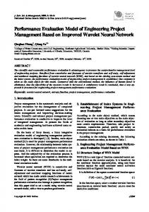
Fig. 1.

Elements of a General Control System

Control theoretic approaches have been successfully applied to selected resource management issues including task scheduling [7], bandwidth allocation, QoS adaptation in web servers [8], multi-tier websites [9], load balancing in e-mail and file servers [9], and processor power management [10]. Control theory provides a systematic way to design an automated and efficient resource management technique by continuous observation of the system state, variation in the environment input, and finite control inputs such that system always operates in a safe and stable state region while maintaining the QoS demands. A typical control system consists of the components shown in Fig. 1. Set Point is the desired state of the system in consideration that a system tries to achieve during its operation. Control Error is the difference between the desired system set point and the measured output during system operation. Control Inputs are the set of system parameters, which are applied to the system dynamically for changing the performance level of the system. The Controller module takes observation of the measured output and provides the optimal combination of different control inputs to achieve the desired set point. Estimator module estimates the unknown parameters for the system based upon the previous history using statistical methods. Disturbance Input can be considered as the environment input that affects the system performance. Target system is the system in consideration, while System Model is the mathematical model of the system, which defines the relation between its input and output variables. A Learning Module takes measured output through the monitor and extracts information based on the statistical methods. System State shows the relationship between control/input variables and performance variables of the system. IV. E XPERIMENTAL S ETUP Our experimental setup consists of four physical nodes: Nop01, Nop02, Nop03 and Nop10. Names Nop04 to Nop09 are reserved for the virtual machines. Table I summarizes configuration of physical machines. Nop03 and Nop10 both have Dynamic Voltage and Frequency Scaling (DVFS) capability that allows administrator to tune the complete physical

Name Nop01

Cores 8

Nop02 Nop03 Nop10

4 8 8

Description 2 Quad core 1.9GHz AMD Opteron 2347 HE 2.0 GHz Intel Xeon E5405 processor 2 Quad core 1.9GHz AMD Opteron 2350 2 Quad core 1.9GHz AMD Opteron 2350z

RAM 8GB

DVFS No

VMs Nop04,Nop07 (Development Machines)

4GB 8GB 8GB

No Yes Yes

Nop05,Nop08 (Client Machines) Nop06,Nop09 (Application server) Nop11,Nop12 (Database Server)

TABLE I P HYSICAL MACHINE CONFIGURATION .

Control Variables CPU Frequency Cap on Virtual machine resources. Load distribution percentage (in a cluster) Number of Service Threads Number of Virtual Machines in Cluster

State Variables CPU Utilization (Observable) Memory Utilization (Observable) Service Time (Unobservable) Queue waiting Time (Unobservable) Queue Size on each server (Unobservable) Number of Live Threads (Observable) Peak Threads available in a JAVA VM (Observable)

Performance Variables Average Response Time Power consumption in Watts %age of Errors

TABLE II S YSTEM PARAMETERS .

node or its individual core for desired performance level. We have used Xen Hypervisor (http://www.xen.org/) and Linux version 2.6.18-92.el5xen to create and manage physical resources (CPU and RAM) for cluster of Virtual Machines (VMs) on these physical servers. Table I also shows the virtual machines (VM) running on all physical machines and the roles played by those VMs. VM Nop06 and Nop09 are running over physical host machine Nop03 while database server VMs Nop11 and Nop12 are running on physical host Nop10. Application server Nop06 is attached to the database server Nop12 and Nop09 is attached to the Nop11. All VM run same version of Linux. Client machines are used to generate request load. Application servers run the open source version of IBM’s J2EE middleware, Web Sphere Application Server Community Edition (WASCE). Database machines run MySQL. Example Application: We used Daytrader, an open source benchmark application developed to compare and measure the performance of multi-tier J2EE web servers in industry, as our web application. Daytrader is available as open source application with WASCE. It drives a trade scenario that allows users to monitor their stock portfolio, inquire about stock quotes, buy or sell stock shares, as well as measure the response time for benchmarking. Out of the box, the Daytrader application puts most of the load on the database server. We modified the main trade scenario servelet to allow shifting the processing load of a request from the database node to the computing node. In the modified daytrader application, for each request, webserver generates a random symbol from the symbol set of available stock names. Webserver performs database query based on that symbol and returns the result of the query to the client. As an added computation on the application server, we perform computation of sum of the first N integer, where N is supplied through the client workload. All client requests contain same N to make them homogeneous in computation nature. This was done to emulate business enterprise loads in highly dynamic environment. For the basic service, we

distributed the Daytrader application across multiple instances of WASCE, deployed over virtual machines ( Nop06 and Nop09). Finally, a modified Daytrader client is used to generate workload requests based on a given throughput profile (specified as a lookup table). This table contains the sampling period and number of requests in that period. Due to limitation of workload pattern (only uniform is allowed) in Daytrader client, we use the Httperf [20] benchmarking application client tool for measuring the web server performance in all of our experiments in following sections. This client tool supports both http 1.0/1.1 and SSL protocols. It provides flexibility to generate various workload patterns (poisson, deterministic, and uniform) with numerous command line options for benchmarking. Similar to the modified Daytrader client, Httperf also generates workload requests based on a given throughput profile (specified as a lookup table). Due to its availability as open source, we have modified it to print the performance measurements of our interest periodically while running the experiment. At the end of each sample period, modified version of Httperf prints out the detailed performance statistics of the experiment in terms of total numbers of requests sent, minimum response time, maximum response time, average response time, total number of errors with types, and response time for each request. Furthermore, to support the high workload between the client - web server interface, changes were made to remove the file socket limitation in the Linux OS installed over client and webserver machines. Monitoring: Specially developed python scripts are used as monitoring sensors on all virtual and physical machines. These sensors monitor CPU, disk and RAM utilization of the node (physical and virtual) throughout the system run and report data after each sampling interval as well as at the end of the experiment. Furthermore, modifications to the web server code allows us to monitor web server performance in terms of max threads active in web server, response time measured at first tier and at the database tier for each incident request, and average queue size after each

sampling interval. The client returns the measured maximum, minimum, and average response time during the sampling period. We have specified 100 seconds as the timeout value for a request response. Any outstanding request after the timeout is logged as an error. It also returns the number of errors with their type (client timeout, connection reset, etc) in each sample. Measurement of power consumption over a physical node is performed with help of a real time watt meter. The average power consumption is measured over a sampling interval of 15 seconds as per the requirements and data is transferred to computer through the interface software over USB. Xenmon [21] is used to measure the virtual CPU utilization at VMs for each sampling interval. Synchronization: System time is synchronized using NTP. The jitter in monitoring sensors across all servers is controlled using a PID controller as described in [22]. V. I DENTIFICATION OF THE S YSTEM PARAMETERS As a result of different experiments described in Section VI, an extensive list of system parameters have been identified, which is shown in Table II. This list contains three different types of parameters: Control Variables, State Variables, and Performance Variables. Control variables can be controlled at runtime during experiment for tuning the system to achieve performance objectives. State variables describes the current state of system under observation. Performance variables are used to quantify QoS objectives. Additionally, state variables are divided into two different categories: Observable and Unobservable. Observable variables can be measured directly through sensors, system calls or application related API, while unobservable variables can not be measured directly, instead they are estimated within certain accuracy using existing measurements through various techniques at runtime. During our experiments, we used specially written sensors or different tools to measure observable variables, while unobservable variables (e.g. service time and delay) are estimated through the exponential Kalman filter described in Section VII-A.

Fig. 2. Power consumption on Nop03 vs CPU frequency and Aggregate CPU core utilization.

VI. S YSTEM M ODELING A PPROACH For identifying an accurate system model of a distributed multi-tier system, extensive experiments have been per-

formed and results have been analyzed. During these experiments, we analyzed the multi-tier system performance with respect to system utilization, various work load profiles, bottleneck resource utilization, and its impact on system performance. Additionally, we calculated work factor of our client requests with help of linear regression techniques described in [23]. details of modeling efforts are described in following sub-sections. A. Model for Power Consumption As a first step towards system model identification, the mutual relationship among physical CPU core utilization, CPU frequency, and power consumption of the physical server is identified. This work is an extension of the power modeling effort described in [1] to model the system power consumption with greater accuracy that can be utilized effectively in real time physical server deployment. Fig. 2 shows the power consumed on one of the physical server Nop03 with respect to the aggregate CPU core usage and CPU frequency. An extensive experiment was performed over physical server Nop03 with help of a specially written script, which exhausted a physical CPU core through floating point operations in increments of 10% utilization independent of the current CPU frequency. With multiple instances of this utility, all eight physical CPU core of the Nop03 server were loaded in incremental manner for different discrete values of CPU frequencies. CPU frequency across all of the physical cores (1 to 8) was kept same during each step. The consumed power was measured with help of a real time watt meter. Based on this experiment, we created a regression model for power consumption at physical machine with respect to CPU core frequency and aggregate CPU utilization. After analysis of the results (and reconfirmation with several other experiments across other nodes), it was observed that power consumption model of a physical machine is non-linear because power consumption in these machines depends not only upon the CPU core frequency and utilization, but also depends non-linearly on other power consuming devices e.g. hard drive, CPU cooling fan etc. As a result, a look-up table with near neighbor interpolation was found to be the best fit for aggregating the power consumption model of the physical machine. Combination of CPU frequency, and aggregate CPU core usage of the physical machine is used as a key of the lookup table to access the corresponding power consumption value. This aggregate power model was utilized further for the controlled experiments described in section VIII. B. Determining Request Characteristics Httperf benchmark application code was modified to allow the generation of client requests to the webserver, N op03, at a pre-specified rate provided from a trace file. At Nop03, each request performed certain fixed floating point computation on the webserver and then performed some random select query on the database machine. To better understand the nature of requests, we performed analysis to compute the number of CPU cycles needed to process the request. This linear regression technique is explained in [23].

Fig. 3.

Fig. 6.

Work factor Plot for Request Characteristic

A queuing model for the two-tier system.

During any sampling interval T , if ρ is virtual CPU utilization, f is CPU frequency, Wf c is the work factor of the request (defined in terms of CPU clock cycles), λ is request rate, and ψ is system noise. Then, ρ ∗ f = λ ∗ Wf c + ψ. The average workfactor was computed to be 2.5X104 CPU cycles with coefficient of variation = 0.5. The variation in Wf c shows the variation in the nature of final request based upon the chosen symbol for query. Result of the experiment is shown in Fig. 3. VII. E XPERIMENT 1: N O C ONTROLLER This experiment was performed to learn the system characteristics, identify bottle necks and have a benchmark to compare the performance of a later experiment in which we used the predictive controller that we developed. This first experiment was configured with Nop09 (physical machine Nop03) as the virtual machine running the first tier of Daytrader application. With help of Xen, virtual CPU of Nop09 was pinned to a single physical core and 50% of the physical core was assigned to Nop09 as maximum available computational resource. Physical memory was also limited to 1000MB for Nop09. Nop11 was configured as database using similar CPU and memory related operating settings over physical server Nop10. To simulate real time load scenario, all CPU cores of physical server Nop03 (except the CPU core hosting Nop09) were loaded approximately 50% with help of utility scripts described in Section VI-A. MAX JAVA threads, a parameter that sets the maximum concurrency limit was configured as 600 in the webserver application. All CPU cores in physical server Nop03 are operating at their maximum frequency 2.0 Ghz. Results of this experiment are

shown in figure( 4 and 5) and prominent observations are listed in following paragraph. Observations from figure( 4 and 5): The aggregate CPU utilization (sub-figure 1) (numbered from top to bottom) and memory utilization (sub-figure 2) of webserver and database tier are shown in Fig. 4. According to sub-figure 1, initial CPU utilization of physical server Nop03 is approximately 46% due to loading of the CPU cores as described in previous paragraph, while addition to the Nop03 CPU utilization is due to contribution of weberser Nop09 during the experiment. Power consumption of the physical machine Nop03 is shown in sub-figure 3 and aggregate utilization of the physical machine Nop03 (similar to Nop03CPU in subfigure 1) is shown in sub-figure 4. Sub-figure 6 represents the java thread utilization of the web server and sub-figure 7 shows the queue size of the web server through the method described in section VIII-A. Distribution of observed response time at webserver is shown in Fig. 5 sub-figure 1 while the min, max, and mean value of response time is plotted in sub-figure 2 of the same figure. Figure 5(sub-figure 3) show the generated client request rate, (ActualRequestRateSent), and corresponding server throughput (ActualRequestRateCompleted) for the experiment. Time series “ExpectedRequestRate” shows the request profile supplied to the client, which can be different from the “ActualRequestRateSent” in case of client side connection limitations. The request trace in these experements was based on the user request traces from the 1998 World Cup Soccer(WCS-98) web site [24]. According to Fig.( 4 and 5), the correlation among request rate (fig 5 sub-figure 3) , CPU utilization (fig 4 sub-figure 1 and 4), and response time (fig 5 sub-figure 1) is apparent. However, Live JAVA threads shown in Fig. 4 sub-figure 6 are not decreasing with decrease in client request rate. Upon investigation we discovered that this is due to the thread pool policy, which does not allow threads to be idle for a time long enough such that they are never retired from the thread pool. However, all live threads in this case are not necessarily actively working. A. Estimating Bottleneck Resource It is important to determine the bottleneck resource in a distributed system. For that purpose, we used a queuing approximation for a two tier system as shown in Fig. 6. λ is the incoming throughput of requests to an application. ρ is the utilization of the bottleneck resource. S is the average service time on the bottleneck resource. D is the average delay. T is the average response time of a request. The average waiting time for a request is W = T − S − D. We define a queue model with state vector [S; D] and observation vector as [T ]. An exponential Kalman filter (KF) was used to estimate the system state as mentioned earlier. It is important to note that we can approximate the system as a M/G/1/∞ PS queue if the system has no bottleneck. In the presence of bottleneck, the system utilization (not necessarily CPU) will approach unity. At that time, the system will change to the LPS queue model. However, as mentioned earlier, it is difficult to build

a tractable model for LPS queuing systems. Hence, we just identify the operating regions where the system changes the mode between two queuing models and analyze the system in the Infinite PS queue region only. The KF equations, written in the term of exponentially transformed variables, [x1 ∈ R; x2 ∈ R] s.t. S = exp(x1) and D = exp(x2) are as follows. Note that this transformation ensures S, D ∈ R+ : For a giventimed  index of observa ˆ k) exp(x1 exp(x1k−1 ) tion, k, the equations = + ˆ k) exp(x2k−1 ) exp(x2 N (0, Q) and T = exp(x1k ) ∗ (1/(1 − λk ∗ exp(x1k ))) + exp(x2k ) + V (0, R) define the state update dynamics and observation. N and V are Gaussian process and measurement noises with mean zero and covariances Q and R respectively. One can verify that these equations described the behavior of a M/G/1 PS queue. Here, predicted bottleneck utilization is given by ρˆk = λk *exp(x1k ). Additionally, the Kalman filter does not update its state when the predicted bottleneck resource utilization becomes more than 1. Observations from figure 7: According to Fig. 7(subfigure 1), the developed exponential Kalman filter tracks service time S and delay D at webserver perfectly with low variance as the experiment (section VII) progresses. Additionally, as per sub-figure 2, Kalman filter tracks bottleneck utilization as similar to CPU utilization of the system. However, we noticed that sometime, the bottleneck utilization might saturate at 1 without the CPU utilization reaching that value. In those cases, we discovered that the number of available system threads acted as the bottleneck. According to sub-figure 3, predicted response time from the Kalman filter Tpred and actual response time T also very close to each other, which indicates efficiency of the Kalman filter. B. Experiment 2: Impact of Maximum Usage of Bottleneck Resource The primary motive for this investigation was to observe the affect of high bottleneck resource usage on system performance. In this case, we chose the settings that made the number of available threads as the system bottleneck. We did various experiments with different setting for Max JAVA Threads. This parameter sets the maximum number of threads that can be used for request processing. Based on our observation, there are typically 90 more system threads which are not accounted under this cap. Fig. 8 shows the results for the one experiment with max threads set to 750. This figure shows that at maximum utilization of the bottleneck resource, system performances decrease significantly and response time from the webserver becomes unpredictable. Furthermore, this is the region, where the system transitions from a PS queue to a LPS queue system. Once the system reaches the max utilization of the bottleneck resources, it restricts entry for more requests into the system resulting into max utilization of the incoming system queue which in turn results in rejection of the incoming client requests from the server. Therefore, to achieve predefined QoS specifications, system should never be allowed to reach the maximum utilization of bottleneck

resource. Additionally, this boundary related to max usage of bottleneck resource can also be considered as “Safe Limit” of system operation. C. Experiment 3: Impact of Limited usage of Bottleneck Resource After determining the bottleneck resource and impact of its maximum utilization over web server performance, next step was to observe the web server performance, when the bottleneck resource utilization varies from minimum to maximum and back to minimum. This type of study provides knowledge regarding web server performance if bottleneck resource utilization is lowered from maximum limit through a controller that maintains the QoS objective of the multi-tier system. The configuration settings for this experiment was same as experiment 1. MAX number of JAVA threads for experiment is 600. The client request trace profile used for this experiment is shown in Fig. 9 subfigure 6 . According to the results shown in the same figure (Fig. 9), system utilization (subfigure 1) and performance in terms of response time (subfigure 4) follows the trend of applied client request profile (sub-figure 6). We can also see the sudden jump in size of server queue (sub-figure 3), which indicates contention of computational resource among all of the pending requests inside the system. Sudden increase in RAM utilization is due to the increase in thread utilization of the system. Additionally, from the comparison of request rate and response time plot in Fig. 9, it is apparent that by lowering the system utilization and client load on the web server, web server can be brought back to state, where it can restore QoS objective of the system that can be consist of minimizing the system queue size and server response time. Kalman Filter Analysis: Results of the experiment were analyzed with the help of Kalman filter described in section VII-A and results of the analysis are shown in Fig 10. According to Fig. 10, the defined exponential Kalman filter tracks service time and delay at webserver quite well with low variance as the experiment progresses. One can notice the regions where the bottleneck resource utilization approaches unity but the CPU utilization is less than one. Upon further investigation of those time samples, the bottleneck resource was found to be the maximum number of Java threads available in webserver. This limit can be changed by the ‘MAX JAVA Threads’ configuration setting. The goal of any successful controller design for performance optimization of the system will be to drive the system to work in the stable region (where the bottleneck resource utilization is less than unity). During the experiment, when predicted utilization of the bottleneck resource is more than one, Kalman filter does not updates its states. VIII. E XPERIMENT 4: W ITH P REDICTIVE C ONTROLLER This section implements the observed system model defined in Section VII-A as an online Kalman filter over multitier system, which predicts the service time (workfactor) Sˆ of the incident requests on the webserver. The predicted

A. The Predictive Controller:

Fig. 11.

Main components of the control structure from section VIII-B

service time Sˆ is used by a Predictive Controller similar to the L0 Controller described in [16] to predict the aggregate response time of the incident requests during the next sample time (look-ahead horizon N ) of the system based on different possible combinations of control inputs (CPU core frequency). Now the predictive controller will choose the best possible control input for the system to achieve the pre-specified QoS objective of the system during next sample interval. The predictive controller tries to optimize the system behavior in terms of QoS objectives by continuous observation of the underlying system and choosing the best control input for the system in next sample interval. Although there are a large number of system parameters listed in section V, but we have chosen a small set of most important parameters for our predictive controller to show the performance of our modeling approach. We have chosen CPU core frequency as the control input due to its impact on the system performance in multiple dimensions for response time of the system and power consumption both. Additionally, system queue size and response time are considered as as state variable for the system due to their ability to show the exact system health. According to the experiments shown in sections VII and VII-C, it is evident that the higher value of application queue represents contention in computational resources of the application and total response time value indicates system’s capability to minimize or process the requests lying in system queue with the new arrived request during that sample period. Therefore, we try to minimize the application queue size and total response time as one of the component in cost function J described in section VIII-A. Response time and power consumption are considered as performance variables, which are used in web service industry to define a typical multidimensional service level agreements (SLAs). We have plan to incorporate other variables also in future implementations of more complex version of the predictive controller. Implementation details of the predictive controller is presented in following subsection.

We developed a JAVATM based predictive controller for adjusting operating frequency of the physical CPU core with respect to varying load conditions. The control structure consists of the following key components: System Model: It identifies the relationship between resident requests (System Queue size) inside the system and total response time to process those requests. The system dynamics is generally defined as follows: x(t + 1) = φ(x(t), u(t), λ(t)), where x(t) is the system state at discrete time sample t, where x(t) ⊂ Rn , u(t) is the control input at time t, where u(t) ⊂ Rm , and λ(t) is the environment input at time t. T is the sampling time of the system. The system state for this experiment, x(t), at time t can be defined as set of system queue q(t) and response time r(t), that is, x(t) = [q(t); r(t)]. The queuing system model ˆ + is given by the equation: qˆ(t + 1) = max{q(t) + (λ(t Wˆf α(t+1) , 1) − Wˆ ) ∗ T, 0} and rˆ(t + 1) = (1 + qˆ(t + 1)) ∗ α(t+1) f where at time t, q(t) is the queue level of the system, λ(t) is the arrival rate of requests, r(t) is the response time of the system, α(t) is a scaling factor defined as u(t)/umax where u(t) is the frequency at time t, umax is the maximum supported frequency in the system, Wˆf is the predicted average service time (work factor in units of time) required per request at the maximum frequency. Online Kalman filter estimates the service time Sˆt of the incident request at current frequency u(t), which is scaled against the maximum supported frequency of the system to calculate the work factor (Wˆf = Sˆt ∗ uu(t) ). Finally, E(t) is the system power max consumption in watts. Use of Request Forecasting Technique: The estimation of future environmental input and corresponding output of the system are crucial for the accuracy of the model. In this experiment, an autoregressive moving average model was used as estimator of the environmental input as per following equation. λ(t + 1) = β ∗ λ(t) + γ ∗ λ(t − 1) + (1 − (β + γ)) ∗ λ(t − 2), where β and γ determines the weight on the current and previous arrival rates for prediction. Control Algorithm and Performance Specification: During a given time t, the controller calculates the optimal value of frequency u(t) for the time interval from t to (t+1) such that the cost function can be minimized.We use a cost function J(t + 1), which is the weighted conjunction of drift from the desired set point xs , of the system state and power consumption E(t + 1). In our experiment, xs = [q∗, r∗] where q∗ = desired maximum queue size, r∗ = desired maximum response time, X = [q, r] is the system state at current time, and J(t + 1) = Q ∗ kX (t + 1) − xs )k + R ∗ kE(t + 1)k, where Q and R are user specified relative weights for the drift from the optimal system state xs and power consumption E(t + 1), respectively. The power consumption E(t + 1) is predicted with the help of lookup table generated in section VI-A based upon the current frequency of the CPU core and aggregate system utilization of the physical server. Starting from a time t0 , the optimization problem for

the controller is to minimize the total cost of operating the system J in future lookahead prediction horizon t = 1...N steps. We chose N = 2 in this experiment. min

U

t=t 0 +1 X

J(x(t), u(t))

t=t0 +N

B. System Model for Predictive Control We used the exponential Kalman filter described earlier to track the system state online. The two main parameters received from the filter are the current service time S and predicted response time Tpred . These values are then plugged into the model described in the previous section. The power model described in Section VI-A was used to estimate the system (physical node of webserver) power consumption. With help of these system and power model, the predictive controller provides the optimal configuration of the system in terms of CPU core frequency. Performance of the online controller directly depends upon the accuracy of Kalman filter estimation of the parameters of the webserver application model and the power consumption model of the physical system. Experiment settings: Experimental settings and incoming request profiles were kept similar to Section VII for direct comparison between the webserver performance with and without the controller implementation. The Controller architecture is shown in Fig. 11. The Local Response Monitor monitors the webserver performance on the VM (Nop09) hosting web server. It collects, processes, and reports performance data after every SAMPLE TIME (in this case it was set to 30 seconds) to the Local Controller running on host machine (Nop03). These performance data includes average service time at webserver (computation time at application tier as well as query time over database tier), average queue size (average resident request into the system) of the system during the time interval of SAMPLE TIME, and request arrival rate. The average queue size of the system is measured based on the total resident request in the system at previous sample, (plus) total incident request into the system, and (minus) total completed request from the system in the current sample duration. Results from the experiment are shown in Fig. 12 and 12, while plots of the estimates from the online Kalman filter are shown in Fig 14. For this experiment, we have chosen optimal system state xs = [q∗, r∗] where q∗ = 0 and r∗ = 0, which shows our inclination towards keeping system queue and response time both minimum. Q and R are assigned values equal to 10000 and 1 respectively to penalize the multi-tier system a lot more for increment in queue size and response time compared to the increment in power consumption. Additionally, look ahead horizon value N is 2 for the current experiment to keep the controller computation simple and efficient. During forecasting of future predicted arrival request rate β and γ were equal to 0.8 and 0.15 respectively to put maximum weight on the current arrival rate to calculate future arrival request rate.

Observations from Figure 12 and Figure 13: The aggregate CPU utilization (sub-figure 1) and memory utilization (sub-figure 2) of webserver and database tier are shown in Fig. 12. Power consumption of the physical machine Nop03 is shown in sub-figure 3 and aggregate utilization of the physical machine Nop03 (similar to Nop03CPU in sub-figure 1) is shown in sub-figure 4. Sub figure 6 represents the java thread utilization of the web server and sub-figure 7 shows the queue size of the web server through the method described in section VIII-A. Distribution of observed response time at webserver is shown in Figure 13 (sub-figure 1) while the min, max, and mean value of response time is plotted in sub-figure 2. Figure 13 (sub-figure 3) shows the generated client request rate, (ActualRequestRateSent), and corresponding server throughput (ActualRequestRateCompleted) for the experiment. Time series “ExpectedRequestRate” shows the request profile supplied to the client, which can be different from the “ActualRequestRateSent” in case of client side connection limitations. The most interesting plot in figure 12 is sub-figure 5, which shows the change in frequency of the CPU core from the controller to achieve predefined Qos requirements based upon the control steps taken by observing the system state and estimating the future environmental inputs. After direct comparison of sub-figure 5 and subfigure 3 from Figure 13, we can see that change in CPU core frequency follow similar trend as incident request rate at web server. Additionally, controller has chosen 1.2 Ghz frequency for the CPU core until there is some sudden increase or decrease in the incident request rate. Furthermore, controller changes frequency of the core very less often even when incident request rate is changing continuously, which shows the minimal disturbance in the system operation due to predictive controller. Comparative analysis of the controller results: Performance of the proposed system model can be measured by direct comparison of the current results (Fig. 12 and 13) with the results from section VII(Fig. 4 and 5). Observation of the plots from both experiments lead to the following observations. According to the Fig. 14, online Kalman filter tracks average response time of the incident requests well. Additionally, it tracks bottleneck utilization with high accuracy. The estimated service time of the incident requests by the Kalman filter shows minimal variation. The controlled version runs at a lower frequency most of the times, which results into considerable amount of power saving (18%) over a period of four hours of experiment (Fig. 12 and 13) compared to the baseline experiment shown in section VII(Fig. 4 and 5). The controller changes the frequency of the CPU core at very few occasions, but it is able to identify the sudden increase in the incident request rate. This feature shows adaptive nature of the controller in case of varying dynamic load conditions. On comparing Fig.( 4 and 5) with Fig.( 12 and 13), it is clearly visible that there is negligible memory overhead due to the controller. Additionally, the overhead in virtual CPU utilization over webserver Nop09 due to controller contributes little to the aggregate system

overhead. The increased virtual CPU utilization can mostly be attributed to the lower physical core frequency. According to Fig. 4 and Fig. 12, even after presence of controller and slow running system, response times at webserver is in the similar range. It shows that controller while managing to decrease power consumption does not affect QoS objectives of the system negatively. According to figure 15, the power model described in section VI-A, estimates the power consumption in the physical machine Nop03 quite well with only 5% average error in prediction that indicates the effectiveness of the power consumption model. Additionally, Java thread utilization is less in case of controller, which indicates that even after slowing down the system, incident requests are getting served in time without much contention of computational resources. Furthermore, mean server queue statistics (Fig. 4 and Fig. 12) are in the same range for both cases. Observations in previous paragraph indicates that the current system model captures the dynamics of the multitier web server (dyatrader) perfectly with high accuracy. Additionally, the system model uses typical control inputs, state variables, and performance measurements of the multitier web service domain for achieving QoS objectives that makes proposed framework suitable for any multi-tier web service system. IX. C ONCLUSION We have presented an approach to develop accurate models for multi-tier enterprise systems. The developed model can be integrated with a predictive control framework for dynamically changing the system tuning parameters based on the estimated time varying workload. The proposed power consumption model of the system is used by the controller to optimize system performance and was able to achieve 18% reduction of power consumption in four hours of experiment. Furthermore, the experimental results indicates that the combined approach has low run-time overhead in terms of computational and memory resources. Acknowledgment This work was supported in part by the NSF SOD Program, contact number CNS-0804230. The authors will also like to acknowledge Manish Khushwaha from Vanderbilt University for his help with the Kalman filter discussions. R EFERENCES [1] Abhishek Dubey, Rajat Mehrotra, Sherif Abdelwahed, and Asser Tantawi. Performance modeling of distributed multi-tier enterprise systems. SIGMETRICS Performance Evaluation Review, 37(2):9–11, 2009. [2] http://aws.amazon.com/ec2/. [3] http://www.google.com/apps/intl/en/business/ index.html. [4] http://www.research.ibm.com/autonomic/. [5] http://www.microsoft.com/presspass/press/2003/ mar03/03-18DynamicSystemsPR.mspx. [6] http://h10134.www1.hp.com/services/ adaptiveinfrastructure/. [7] Anton Cervin, Johan Eker, Bo Bernhardsson, and Karl-Erik AArz´en. Feedback–feedforward scheduling of control tasks. Real-Time Syst., 23(1/2):25–53, 2002.

[8] T.F. Abdelzaher, K.G. Shin, and N. Bhatti. Performance guarantees for web server end-systems: a control-theoretical approach. Parallel and Distributed Systems, IEEE Transactions on, 13(1):80–96, Jan 2002. [9] Chenyang Lu, Guillermo A. Alvarez, and John Wilkes. Aqueduct: Online data migration with performance guarantees. In FAST ’02: Proceedings of the 1st USENIX Conference on File and Storage Technologies, page 21, Berkeley, CA, USA, 2002. USENIX Association. [10] Dara Kusic, Nagarajan Kandasamy, and Guofei Jiang. Approximation modeling for the online performance management of distributed computing systems. In ICAC ’07: Proceedings of the Fourth International Conference on Autonomic Computing, page 23, Washington, DC, USA, 2007. IEEE Computer Society. [11] Chenyang Lu et al. Feedback control real-time scheduling: Framework, modeling and algorithms. Journal of Real-Time Systems, 23:85– 126, 2002. [12] T. Simunic and S. Boyd. Managing power consumption in networks on chips. In Proc. Design, Automation, & Test Europe (DATE), pages 110–116, 2002. [13] Chi-Hong Hwang and Allen C.-H. Wu. A predictive system shutdown method for energy saving of event-driven computation. ACM Trans. Des. Autom. Electron. Syst., 5(2):226–241, 2000. [14] Jonathan Wildstrom, Peter Stone, Emmett Witchel, Raymond J. Mooney, and Mike Dahlin. Towards self-configuring hardware for distributed computer systems. In The Second International Conference on Autonomic Computing, pages 241–249, June 2005. [15] Yixin Diao, Joseph L. Hellerstein, Sujay Parekh, Hidayatullah Shaikh, Maheswaran Surendra, and Asser Tantawi. Modeling differentiated services of multi-tier web applications. In MASCOTS ’06, pages 314– 326, 2006. [16] N. Kandasamy, S. Abdelwahed, and M. Khandekar. A hierarchical optimization framework for autonomic performance management of distributed computing systems. In Proc. 26th IEEE Int’l Conf. Distributed Computing Systems (ICDCS), 2006. [17] Leonard Kleinrock. Theory, Volume 1, Queueing Systems. WileyInterscience, 1975. [18] R. E. Kalman. A new approach to linear filtering and prediction problems. Transactions of the ASME Journal of Basic Engineering, 82(Series D):35–45, 1960. [19] Evangelia Kalyvianaki, Themistoklis Charalambous, and Steven Hand. Self-adaptive and self-configured cpu resource provisioning for virtualized servers using kalman filters. In ICAC ’09: Proceedings of the 6th international conference on Autonomic computing, pages 117–126, New York, NY, USA, 2009. ACM. [20] HP. httperf documentation. Technical report, 2007. [21] Diwaker Gupta, Rob Gardner, and Ludmila Cherkasova. Xenmon: Qos monitoring and performance profiling tool. Technical report, HP Labs, 2005. [22] Abhishek Dubey et al. Compensating for timing jitter in computing systems with general-purpose operating systems. In ISROC, Tokyo, Japan, 2009. [23] Giovanni Pacifici, Wolfgang Segmuller, Mike Spreitzer, and Asser Tantawi. Dynamic estimation of cpu demand of web traffic. In valuetools ’06: Proceedings of the 1st international conference on Performance evaluation methodolgies and tools, page 26, New York, NY, USA, 2006. ACM. [24] M. Arlitt and T. Jin. Workload characterization of the 1998 world cup web site. Technical Report HPL-99-35R1, Hewlett-Packard Labs, September 1999.

Fig. 4.

Web server behavior from section VII: Sampling period=30 seconds.

Fig. 5.

Web server behavior from section VII: Sampling period=30 seconds.

Fig. 7. Offline Exponential Kalman filter output corresponding to the results from section VII (Fig. 4). Service time and delay are in millisecond range. Response time is specified in seconds.

Fig. 8.

Impact of Max utilization of bottleneck Resource on performance from section VII-B. MAX Thread =750.

Fig. 9.

Web Server Behavior While Limiting the Use of Bottleneck Resource from section VII-C.

Fig. 10. Offline KF Analysis of the results from Fig. 9 of section VII-C. Service time and delay are in milliseconds. Response time is specified in seconds.

Fig. 12.

Web server behavior With Controller as per section VIII-B: Sampling period=30 seconds.

Fig. 13.

Web server behavior With Controller as per section VIII-B: Sampling period=30 seconds.

Fig. 14. Online exponential Kalman filter output corresponding to the experiment from Section VIII-B (figure 12 and 13). Service time and delay are in millisecond range. Response time is specified in seconds.

(a) Predicted and actual Power Consumption in web server from section (b) Error in predicting power consumption compared to actual in secVIII-B tion VIII-B Fig. 15.

Comparison of Power Consumption for Actual Vs predicted through Predictive Controller in section VIII-B.