Model Reduction Based on Spectral Projection ... - Semantic Scholar

Model Reduction Based on Spectral Projection Methods Peter Benner∗

Enrique S. Quintana-Ort´ı† April 8, 2005

Abstract We discuss the efficient implementation of model reduction methods such as modal truncation, balanced truncation, and other balancing-related truncation techniques, employing the idea of spectral projection. Mostly, we will be concerned with the sign function method which serves as the major computational tool of most of the discussed algorithms for computing reduced-order models. Implementations for large-scale problems based on parallelization or formatted arithmetic will also be discussed. This chapter can also serve as a tutorial on Gramian-based model reduction using spectral projection methods.

1

Introduction

Consider the linear, time-invariant (LTI) system x(t) ˙ = Ax(t) + Bu(t), y(t) = Cx(t) + Du(t),

t > 0, t ≥ 0,

x(0) = x0 ,

(1)

where A ∈ Rn×n is the state matrix, B ∈ Rn×m , C ∈ Rp×n , D ∈ Rp×m , and x0 ∈ Rn is the initial state of the system. Here, n is the order (or state-space dimension) of the system. The associated transfer function matrix (TFM) obtained from taking Laplace transforms in (1) and assuming x0 = 0 is G(s) = C(sI − A)−1 B + D. (2) In model reduction we are faced with the problem of finding a reduced-order LTI system, ˆx(t) + B ˆu x ˆ˙ (t) = Aˆ ˆ(t), ˆ ˆ yˆ(t) = C x ˆ(t) + Dˆ u(t),

t>0 t ≥ 0,

x ˆ(0) = x ˆ0 ,

(3)

ˆ ˆ ˆ −1 B ˆ +D ˆ which approximates G(s). of order r, r ≪ n, and associated TFM G(s) = C(sI − A) Model reduction of discrete-time LTI systems can be formulated in an analogous manner; see, e.g., [OA01]. Most of the methods and approaches discussed here carry over to the discretetime setting as well. Here, we will focus our attention on the continuous-time setting, the discrete-time case being discussed in detail in [BQQ03a]. Balancing-related model reduction methods are based on finding an appropriate coordinate system for the state-space in which the chosen Gramian matrices of the system are ∗

Fakult¨ at f¨ ur Mathematik, TU Chemnitz, 09107 Chemnitz, Germany; [email protected]. † Departamento de Ingenier´ıa y Ciencia de Computadores, Universidad Jaume I, 12.071-Castell´ on, Spain; [email protected].

1

diagonal and equal. In the simplest case of balanced truncation, the controllability Gramian Wc and the observability Gramian Wo are used. These Gramians are given by the solutions of the two dual Lyapunov equations AWc + Wc AT + BB T

AT Wo + Wo A + C T C = 0.

= 0,

(4)

After changing to the coordinate system giving rise to diagonal Gramians with positive decreasing diagonal entries, which are called the Hankel singular values (HSVs) of the system, the reduced-order model is obtained by truncating the states corresponding to the n − r smallest HSVs. Balanced truncation and its relatives such as singular perturbation approximation, stochastic truncation, etc., are the most popular model reduction techniques used in control theory. The advantages of these methods, guaranteed preservation of several system properties like stability and passivity, as well as the existence of computable error bounds that permit an adaptive selection of the order of the reduced-order model, are unmatched by any other approach. However, thus far, in many other engineering disciplines the use of balanced truncation and other related methods has not been considered feasible due to its computational complexity. Quite often, these disciplines have a preferred model reduction technique as modal analysis and Guyan reduction in structural dynamics, proper orthogonal decomposition (POD) in computational fluid dynamics, Pad´e and Pad´e-like approximation techniques based on Krylov subspace methods in circuit simulation and microsystem technology, etc. A goal of this tutorial is to convince the reader that balanced truncation and its relatives are viable alternatives in many of these areas if efficient algorithms from numerical linear algebra are employed and/or basic level parallel computing facilities are available. The ideas presented in this paper are part of an ongoing effort to facilitate the use of balancing-related model reduction methods in large-scale problems arising in the control of partial differential equations, the simulation of VLSI and ULSI circuits, the generation of compact models in microsystems, and other engineering disciplines. This effort mainly involves breaking the O(n2 ) memory and O(n3 ) flops (floating-point arithmetic operations) barriers. Several issues related to this challenge are addressed in this paper. By working with (approximations of) the full-rank factors of the system Gramians rather than using Cholesky factors as in previous balanced truncation algorithms, the complexity of all remaining calculations following the computation of the factors of the Gramians usually only grows linearly with the dimension of the state-space. This idea is pursued in several approaches that essentially only differ in the way the factors of the Gramians are computed. Approximation methods suitable for sparse systems based mainly on Smith- and ADI-type methods are discussed in Chapters [GL05] and [MS05]. These allow the computation of the factors at a computational cost and a memory requirement proportional to the number of nonzeros in A. Thus, implementations of balanced truncation based on these ideas are in the same complexity class as Pad´e-approximation and POD. In this chapter, we focus on the computation of full-rank factors of the Gramians by the sign function method which is based on spectral projection techniques. This does not lead immediately to a reduced overall complexity of the induced balanced truncation algorithm as we deal with general dense systems. However, for special classes of dense problems, a linear-polylogarithmic complexity can be achieved by employing hierarchical matrix structures and the related formatted arithmetic. For the general case, the O(n2 ) memory and O(n3 ) flops complexity remains, but the resulting algorithms are perfectly suited for parallel computations and are highly efficient on current desktops or clusters 2

of workstations. Provided efficient parallel computational kernels for the necessary linear algebra operations are available, balanced truncation can be applied to systems with statespace dimension n = O(104 ) and dense A-matrix on commodity clusters. By re-using these efficient parallel kernels for computing reduced-order models with a sign function-based implementation of balanced truncation, the application of many other related model reduction methods to large-scale, dense systems becomes feasible. We briefly describe some of the related techniques in this chapter, particularly we discuss sign function-based implementations of the following methods: – balanced truncation, – singular perturbation approximation, – optimal Hankel norm approximation, – balanced stochastic truncation, and – truncation methods based on positive real, bounded real, and LQG balancing, for stable systems. Using a specialized algorithm for the additive decomposition of transfer functions, again based on spectral projection techniques, all the above balancing-related model reduction techniques can also be applied to unstable systems. At this point, we would also like to mention that the same ideas can be applied to balanced truncation for descriptor systems, as described in Chapter [MS05]—for preliminary results see [BQQ04c]—but we will not elaborate on this as this is mostly work in progress. This paper is organized as follows. In Section 2 we provide the necessary background from system and realization theory. Spectral projection, which is the basis for many of the methods described in this chapter, is presented in Section 3. Model reduction methods for stable systems of the form (1) based on these ideas are described in Section 4, where we also include modal truncation for historical reasons. The basic ideas needed to apply balanced truncation and its relatives to large-scale systems are summarized in Section 5. Conclusions and open problems are given in Section 6. Throughout this paper, we will use In for the identity matrix in Rn×n and I for the identity when the order is obvious from the context, Λ (A) will denote the spectrum of the matrix A. Usually, capital letters will be used for matrices; lower case letters will stand for vectors with the exception of t denoting time, and i, j, k, m, n, p, r, s employed for integers such as indices and dimensions; Greek letters will be used for other scalars; and calligraphic letters will indicate vector and function spaces. Without further explanation, Π will always denote a permutation matrix of a suitable dimension, usually resulting from row or column pivoting in factorization algorithms. The left and right (open) √ complex half planes will be denoted by C− and C+ , respectively, and we will write  for −1.

2

System-Theoretic Background

In this section, we introduce some basic notation and properties of LTI systems used throughout this paper. More detailed introductions to LTI systems can be found in many textbooks [GL95, Son98, ZDG96] or handbooks [Lev96, Mut99]. We essentially follow these references here without further citations, but many other sources can be used for a good overview on the subjects covered in this section. 3

2.1

Linear Systems, Frequency Domain, and Norms

An LTI system is (Lyapunov or exponentially) stable if all its poles are in the left half plane. Sufficient for this is that A is stable (or Hurwitz ), i.e., the spectrum of A, denoted by Λ (A), satisfies Λ (A) ⊂ C− . It should be noted that the relation between the controllability and observability Gramians of an LTI system and the solutions of the Lyapunov equations in (4) only holds if A is stable. The particular model imposed by (1), given by a differential equation describing the behavior of the states x and an algebraic equation describing the outputs y is called a statespace representation. Alternatively, the relation between inputs and outputs can also be described in the frequency domain by an algebraic expression. Applying the Laplace transform to the two equations in (1), and denoting the transformed arguments as x(s), y(s), u(s) where s is the Laplace variable, we obtain sx(s) − x(0) = Ax(s) + Bu(s),

y(s) = Cx(s) + Du(s).

By solving for x(s) in the first equation and inserting this into the second equation, we obtain ¡ ¢ y(s) = C(sIn − A)−1 B + D u(s) + C(sIn − A)−1 x0 . For a zero initial state, the relation between inputs and outputs is therefore completely described by the transfer function G(s) := C(sIn − A)−1 B + D.

(5)

Many interesting characteristics of an LTI system are obtained by evaluating G(s) on the positive imaginary axis, that is, setting s = ω. In this context, ω can be interpreted as the operating frequency of the LTI system. A stable transfer function defines a mapping G : L2 → L2 : u → y = Gu

(6)

where the two function spaces denoted by L2 are actually different spaces and should more appropriately be denoted by L2 (Cm ) and L2 (Cp ), respectively. As the dimension of the underlying spaces will always be clear from the context, i.e., the dimension of the transfer function matrix G(s) or the dimension of input and output spaces, we allow ourselves the more sloppy notation used in (6). The function space L2 contains the square integrable functions in the frequency domain, obtained via the Laplace transform of the square integrable functions in the time domain, usually denoted as L2 (−∞, ∞). The L2 -functions that are analytic in the open right half plane C+ form the Hardy space H2 . Note that H2 is a closed subspace of L2 . Under the Laplace transform L2 and H2 are isometric isomorphic to L2 (−∞, ∞) and L2 [0, ∞), respectively. (This is essentially the Paley-Wiener Theorem which is the Laplace transform analog of Parseval’s identity for the Fourier transform.) Therefore it is clear that the frequency domain spaces H2 and L2 can be endowed with the corresponding norms from their time domain counterparts. Due to this isometry, our notation will not distinguish between norms for the different spaces so that we will denote by kf k2 the induced 2-norm on any of the spaces L2 (−∞, ∞), L2 , L2 [0, ∞), and H2 . Using the definition (6), it is therefore possible to define an operator norm for G by kGk := sup kGuk2 . kuk2 ≤1

4

It turns out that this operator norm equals the L∞ -norm of the transfer function G, which for rational transfer functions can be defined as kGk∞ := sup σmax (G(ω)).

(7)

ω∈R

The p × m-matrix-valued functions G for which kGk∞ is bounded, i.e., those essentially bounded on the imaginary axis, form the function space L∞ . The subset of L∞ containing all p × m-matrix-valued functions that are analytical and bounded in C+ form the Hardy space H∞ . As a consequence of the maximum modulus theorem, H∞ functions must be bounded on the imaginary axis so that the essential supremum in (7) simplifies to a supremum for rational functions G. Thus, the H∞ -norm of the rational transfer function G ∈ H∞ can be defined as kGk∞ := sup σmax (G(ω)). (8) ω∈R

A fact that will be of major importance throughout this paper is that the transfer function of a stable LTI system is rational with no poles in the closed right-half plane. Thus, G ∈ H∞ for all stable LTI systems. Although the notation is somewhat misleading, the H∞ -norm is the 2-induced operator norm. Hence the sub-multiplicativity condition kyk2 ≤ kGk∞ kuk2

(9)

holds. This inequality implies an important way to tackle the model reduction problem: suppose the original system and the reduced-order model (3) are driven by the same input function u ∈ H2 , so that ˆ yˆ(s) = G(s)u(s),

y(s) = G(s)u(s),

ˆ is the transfer function corresponding to (3); then we obtain the error bound where G ˆ ∞ kuk2 . ky − yˆk2 ≤ kG − Gk

(10)

Due to the aforementioned Paley-Wiener theorem, this bound holds in the frequency domain and the time domain. Therefore a goal of model reduction is to compute the reduced-order ˆ ∞ is smaller than a given tolerance threshold. model so that kG − Gk

2.2

Balanced Realizations

A realization of an LTI system is the set of the four matrices (A, B, C, D) ∈ Rn×n × Rn×m × Rp×n × Rp×m corresponding to (1). In general, an LTI system has infinitely many realizations as its transfer function is invariant under state-space transformations, ½ x → T x, (11) T : (A, B, C, D) → (T AT −1 , T B, CT −1 , D), as the simple calculation D + (CT −1 )(sI − T AT −1 )−1 (T B) = C(sIn − A)−1 B + D = G(s) 5

demonstrates. But this is not the only non-uniqueness associated to LTI system representations. Any addition of states that does not influence the input-output relation, meaning that for the same input u the same output y is achieved, leads to a realization of the same LTI system. Two simple examples are " #· · ¸ ¸ · ¸ · ¸ A 0 £ ¤ x d x x B = + u(t), y(t) = C 0 + Du(t), x1 B1 x1 dt x1 0 A1 " #· · ¸ ¸ · ¸ · ¸ A 0 £ ¤ x d x x B = + u(t), y(t) = C C2 + Du(t), x2 0 x2 dt x2 0 A2 for arbitrary matrices Aj ∈ Rnj ×nj , j = 1, 2, B1 ∈ Rn1 ×m , C2 ∈ Rp×n2 and any n1 , n2 ∈ N. An easy calculation shows that both of these systems have the same transfer function G(s) as (1) so that # · ! # · ! Ã" Ã" ¸ ¸ A 0 A 0 ¤ £ £ ¤ B B , , C C2 , D , , C 0 ,D , (A, B, C, D), 0 B1 0 A2 0 A1 are both realizations of the same LTI system described by the transfer function G(s) in (5). Therefore, the order n of a system can be arbitrarily enlarged without changing the inputoutput mapping. On the other hand, for each system there exists a unique minimal number of states which is necessary to describe the input-output behavior completely. This number n ˆ is ˆ B, ˆ C, ˆ D) ˆ called the McMillan degree of the system. A minimal realization is a realization (A, of the system with order n ˆ . Note that only the McMillan degree is unique; any state-space transformation (11) leads to another minimal realization of the same system. Finding a minimal realization for a given system can be considered as a first step of model reduction as redundant (non-minimal) states are removed from the system. Sometimes this is part of a model reduction procedure, e.g. optimal Hankel norm approximation, and can be achieved via balanced truncation. Although realizations are highly non-unique, stable LTI systems have a set of invariants with respect to state-space transformations that provide a good motivation for finding reduced-order models. From Lyapunov stability theory (see, e.g., [LT85, Chapter 13]) it is clear that for stable A, the Lyapunov equations in (4) have unique positive semidefinite solutions Wc and Wo . These solutions define the controllability Gramian (Wc ) and observability Gramian (Wo ) of the system. If Wc is positive definite, then the system is controllable and if Wo is positive definite, the system is observable. Controllability plus observability is equivalent to minimality of the system so that for minimal systems, all eigenvalues of the product Wc Wo are strictly positive real numbers. The square roots of these eigenvalues, denoted in decreasing order by σ1 ≥ σ2 ≥ . . . ≥ σn > 0, are known as the Hankel singular values (HSVs) of the LTI system and are invariants of the system: let ˆ B, ˆ C, ˆ D) = (T AT −1 , T B, CT −1 , D) (A, be the transformed realization with associated controllability Lyapunov equation ˆc + W ˆ c AˆT + B ˆB ˆ T = T AT −1 W ˆc + W ˆ c T −T AT T T + T BB T T T . 0 = AˆW 6

This is equivalent to ˆ c T −T ) + (T −1 W ˆ c T −T )AT + BB T . 0 = A(T −1 W The uniqueness of the solution of the Lyapunov equation (see, e.g., [LT85]) implies that ˆ c = T Wc T T and, analogously, W ˆ o = T −T Wo T −1 . Therefore, W ˆ cW ˆ o = T Wc Wo T −1 , W ˆ cW ˆ o ) = Λ (Wc Wo ) = {σ 2 , . . . , σn2 }. Note that extending the state-space showing that Λ (W 1 by non-minimal states only adds HSVs of magnitude equal to zero, while the non-zero HSVs remain unchanged. An important (and name-inducing) type of realizations are balanced realizations. A realization (A, B, C, D) is called balanced iff   σ1   .. Wc = Wo =  ; . σn

that is, the controllability and observability Gramians are diagonal and equal with the decreasing HSVs on their respective diagonal entries. For a minimal realization there always exists a balancing state-space transformation of the form (11) with nonsingular matrix Tb ∈ Rn×n ; for non-minimal systems the Gramians can also be transformed into diagonal matrices with the leading n ˆ×n ˆ submatrices equal to diag(σ1 , . . . , σnˆ ), and ˆ cW ˆ o = diag(σ12 , . . . , σ 2 , 0, . . . , 0); W n ˆ

see, e.g., [TP87]. Using a balanced realization obtained via the transformation matrix Tb , the HSVs allow an energy interpretation of the states; see also [Van00] for a nice treatment of this subject. Specifically, the minimal energy needed to reach x0 is inf

u∈L2 (−∞,0] x(0)=x0

Z

0

−∞

ˆ c−1 x u(t)T u(t) dt = (x0 )T Wc−1 x0 = (ˆ x0 )T W ˆ0 =

n X 1 2 x ˆ , σk k k=1



 x ˆ1   where x ˆ0 :=  ...  = Tb x0 ; hence small HSVs correspond to states that are difficult to x ˆn reach. The output energy resulting from an initial state x0 and u(t) ≡ 0 for t > 0 is given by kyk22 =

Z

∞ 0

ˆo x y(t)T y(t) dt = xT0 Wo x0 = (ˆ x0 )T W ˆ0 . =

n X

σk x ˆ2j ;

k=1

hence large HSVs correspond to the states containing most of the energy in the system. The energy transfer from past inputs to future outputs can be computed via E :=

sup u∈L2 (−∞,0] x(0)=x0

R0

kyk22 u(t)T u(t) dt

1

1

¯0 (x0 )T Wo x0 (¯ x0 )T Wc2 Wo Wc2 x , = 0 T −1 0 = (¯ x0 )T x ¯0 (x ) Wc x

−∞

7

where

x ¯0

:=

−1 Wc 2 x0 .

1 2

Thus, the HSVs (Λ (Wc Wo )) =

µ

¶1 2 Λ (Wc Wo Wc ) measure how much 1 2

1 2

the states are involved in the energy transfer from inputs to outputs. In summary, it seems reasonable to obtain a reduced-order model by removing the least controllable states, keeping the states containing the major part of the system energy as these are the ones which are most involved in the energy transfer from inputs to outputs—that is, keeping the states corresponding to the largest HSVs. This is exactly the idea of balanced truncation, to be outlined in Section 4.2.

3

Spectral Projection Methods

In this section we will give the necessary background on spectral projection methods and the related computational tools leading to easy-to-implement and easy-to-parallelize iterative methods. These iterative methods will form the backbone of all the model reduction methods discussed in the next section.

3.1

Spectral Projectors

First, we give some fundamental definitions and properties of projection matrices. Definition 3.1 A matrix P ∈ Rn×n is a projector (onto a subspace S ⊂ Rn ) if range (P ) = S and P 2 = P . Definition 3.2 Let Z ∈ Rn×n with Λ (Z) = Λ1 ∪ Λ2 , Λ1 ∩ Λ2 = ∅, and let S1 be the (right) Z-invariant subspace corresponding to Λ1 . Then a projector onto S1 is called a spectral projector. From this definition we obtain the following properties of spectral projectors. Lemma 3.3 Let Z ∈ Rn×n be as in Definition 3.2, and let P ∈ Rn×n be a spectral projector onto the right Z-invariant subspace corresponding to Λ1 . Then a) rank (P ) = |Λ1 | =: k, b) range (P ) = range (ZP ), c) ker(P ) = range (I − P ), range (P ) = ker(I − P ), d) I − P is a spectral projector onto the right Z-invariant subspace corresponding to Λ2 . Given a spectral projector P we can compute an orthogonal basis for the corresponding Z-invariant subspace S1 and a spectral or block decomposition of Z in the following way: let  " #  R11 R12 , P = QRΠ, R = = @ R11 ∈ Rk×k , 0 0

be a QR decomposition with column pivoting (or a rank-revealing QR decomposition (RRQR)) [GV96] where Π is a permutation matrix. Then the first k columns of Q form an orthonormal basis for S1 and we can transform Z to block-triangular form " # Z11 Z12 T Z˜ := Q ZQ = , (12) 0 Z22 8

where Λ (Z11 ) = Λ1 , Λ (Z22 ) = Λ2 . The block decomposition given in (12) will prove very useful in what follows.

3.2

The Sign Function Method

n×n with no eigenvalues on the imaginary axis, that is, Λ (Z)∩R = ∅, Consider a matrix h −Z ∈ iR and let Z = S J0 J0+ S −1 be its Jordan decomposition. Here, the Jordan blocks in J − ∈

Rk×k and J + ∈ R(n−k)×(n−k) contain, respectively, the stable andiunstable parts of Λ (Z). h −Ik 0 The matrix sign function of Z is defined as sign (Z) := S 0 In−k S −1 . Note that sign (Z) is unique and independent of the order of the eigenvalues in the Jordan decomposition of Z, see, e.g., [LR95]. Many other definitions of the sign function can be given; see [KL95] for an overview. Some important properties of the matrix sign function are summarized in the following lemma. Lemma 3.4 Let Z ∈ Rn×n with Λ (Z) ∩ R = ∅. Then: a) (sign (Z))2 = In , i.e., sign (Z) is a square root of the identity matrix; ¡ ¢ b) sign T −1 ZT = T −1 sign (Z) T for all nonsingular T ∈ Rn×n ; ¡ ¢ c) sign Z T = sign (Z)T .

d) Let p+ and p− be the numbers of eigenvalues of Z with positive and negative real part, respectively. Then 1 p+ = (n + tr (sign (Z))), 2

1 p− = (n − tr (sign (Z))). 2

(Here, tr (M ) denotes the trace of the matrix M .) e) Let Z be stable, then sign (Z) = −In ,

sign (−Z) = In .

Applying Newton’s root-finding iteration to Z 2 = In , where the starting point is chosen as Z, we obtain the Newton iteration for the matrix sign function: Z0 ← Z,

1 Zj+1 ← (Zj + Zj−1 ), 2

j = 0, 1, 2, . . . .

(13)

Under the given assumptions, the sequence {Zj }∞ j=0 converges with an ultimately quadratic convergence rate and sign (Z) = lim Zj ; j→∞

see [Rob80]. As the initial convergence may be slow, the use of acceleration techniques is recommended. There are several acceleration schemes proposed in the literature, a thorough discussion can be found in [KL92], and a survey and comparison of different schemes is given in [BD93]. For accelerating (13), in each step Zj is replaced by γ1j Zj , where the most prominent choices for γj are briefly discussed in the sequel.

9

Determinantal scaling [Bye87]: here, 1

γj = | det (Zj )| n . This choice minimizes the distance of the geometric mean of the eigenvalues of Zj from 1. Note that the determinant det (Zj ) is a by-product of the computations required to implement (13). Norm scaling [Hig86]: here cj =

s

kZj k2 , kZj−1 k2

which has certain minimization properties in the context of computing polar decompositions. It is also beneficial regarding rounding errors as it equalizes the norms of the two addends in the finite-norm calculation ( γ1j Zj ) + ( γ1j Zj )−1 . Approximate norm scaling: as the spectral norm is expensive to calculate, it is suggested in [Hig86, KL92] to approximate this norm by the Frobenius norm or to use the bound (see, e.g., [GV96]) q kZj k2 ≤

kZj k1 kZj k∞ .

(14)

Numerical experiments and partial analytic considerations [BQQ04d] suggest that norm scaling is to be preferred in the situations most frequently encountered in the sign function-based calculations discussed in the following; see also Example 3.6 below. Moreover, the Frobenius norm approximation usually yields a better approximation than the one given by (14). As the computation of the Frobenius norm parallelizes very well, we will mostly use the Frobenius norm scaling in the algorithms based on (13). There are also plenty of other iterative schemes for computing the sign function; many of those have good properties regarding convergence and parallelization (see [KL95] for an overview). Nevertheless, the basic Newton iteration (13) appears to yield the most robust implementation and the fastest execution times, both in serial and parallel implementations. Implementing (13) only requires computing matrix sums and inverses using LU factorization or Gauß-Jordan elimination. These operations are efficiently implemented in many software packages for serial and parallel computations; efficient parallelization of the matrix sign function has been reported, e.g., in [BDD+ 97, HQSW00]. Computations based on the matrix sign function can be considered as spectral projection methods as they usually involve 1 P− := (In − sign (Z)), 2

(15)

which is a spectral projector onto the stable Z-invariant subspace. Also, P+ := (In + sign (Z))/2 is a spectral projector onto the Z-invariant subspace corresponding to the eigenvalues in the open right half plane. But note that P− and P+ are not orthogonal projectors, but skew projectors along the complementary Z-invariant subspace. Remark 3.5 The matrix sign function is criticized for several reasons, the most prominent one being the need to compute an explicit inverse in each step. Of course, it is undefined for matrices with purely imaginary eigenvalues and hence suffers from numerical problems 10

in the presence of eigenvalues close to the imaginary axis. But numerical instabilities basically only show up if there exist eigenvalues with imaginary parts of magnitude less than the square root of the machine precision. Hence, significant problems can be expected in double precision arithmetic (as used in Matlab) for imaginary parts of magnitude less than 10−8 . (A thorough numerical analysis requires the condition of the stable subspace which is given by the reciprocal of the separation of stable and anti-stable invariant subspaces, though—the distance of eigenvalues to the imaginary axis is only an upper bound for the separation!) Fortunately, in the control applications considered here, poles are usually further apart from the imaginary axis. On the other hand, if we have no problems with the spectral dichotomy, then the sign function method solves a problem that is usually better conditioned than the Schur vector approach as it only separates the stable from the anti-stable subspace while the Schur vector method essentially requires to separate n subspaces from each other. For a thorough analysis of sign function-based computation of invariant subspaces, see [BD98, BHM97]. The difference in the conditioning of the Schur form and a block triangular form (as computed by the sign function) is discussed in [KMP01]. Moreover, in the applications considered here, mostly cond (sign (Z)) = 1 as Z is stable or anti-stable, hence the computation of sign (Z) itself is a well-conditioned problem! Therefore, counter to intuition, it should not be surprising that often, results computed by the sign function method are more accurate than those obtained by using Schur-type decompositions; see, e.g., [BQ99]. Example 3.6 A typical convergence history (based on kZj − sign (Z) kF ) is displayed in Figure 1, showing the fast quadratic convergence rate. Here, we computed the sign function of a dense matrix A coming from transforming a generalized state-space system (the n = 1357 case of the steel cooling problem described in Chapter [BS05] of this book) to standard statespace form. We compare the determinantal scaling and the Frobenius norm scaling. Here, the eigenvalue of A closest to R is ≈ 6.7·10−6 and the eigenvalue of largest magnitude is ≈ −5.8. Therefore the condition of A is about 106 . Obviously, norm scaling performs much better for this example. This is a typical behavior for problems with real spectrum. The computations were done using Matlab 7.0.1 on a Intel Pentium M processor at 1.4 GHz with 512 MBytes of RAM.

3.3

Solving Linear Matrix Equations with the Sign Function Method

In 1971, Roberts [Rob80] introduced the matrix sign function and showed how to solve Sylvester and Lyapunov equations. This was re-discovered several times; see [BD75, DB76, HMW77]. We will briefly review the method for Sylvester equations and will then discuss some improvements useful for model reduction applications. Consider the Sylvester equation AX + XB + W = 0,

A ∈ Rn×n , B ∈ Rm×m , W ∈ Rn×m ,

(16)

with Λ (A)∩Λ (−B) = ∅. The latter assumption is equivalent to (16) having a unique solution [LT85]. Let X ∈ Rn×m be this unique solution. Then the straightforward calculation " #" #" # " # In 0 A 0 In 0 A 0 = (17) X Im W −B −X Im 0 −B 11

5

10

0

|| Aj + In ||F

10

−5

10

−10

10

−15

10

Frobenius norm scaling determinantal scaling

−20

10

0

2

4

6

8

10

12

14

16

iteration number (j)

Figure 1: Example 3.6, convergence history for sign (Z) using (13). i h i h In A 0 reveals that the columns of −X span the invariant subspace of Z := W −B corresponding ∗ to Λ (A). In principle, this subspace, and after an appropriate change of basis, also the solution matrix X, can be computed from a spectral projector onto this Z-invariant subspace. The sign function is an appropriate tool for this whenever A, B are stable as in this case, P− from (15) is the required spectral projector. A closer inspection of (13) applied to Z shows that we do not even have to form P− in this case, as the solution can be directly read off the matrix sign (Z): using (17) and Lemma 3.4 reveals that # #! " Ã" −In 0 A 0 = sign (Z) = sign 2X Im W −B so that the solution of (16) is given as the lower left block of the limit of (13), divided by 2. Moreover, the block-triangular structure of Z allows to decouple (13) as A0 ← A, B0 ← B, W0 ← W, for j = 0, 1, 2, . . . ´ 1 ³ Aj+1 ← Aj + γj2 A−1 , j 2γj ³ ´ 1 Bj+1 ← Bj + γj2 Bj−1 , 2γj ´ 1 ³ −1 Wj + γj2 A−1 W B . Wj+1 ← j j j 2γj

(18)

so that X∗ = 21 limj→∞ Wj . As A, B are assumed to be stable, Aj tends to −In and Bj tends to −Im so that we can base a stopping criterion on max{kAj + In k, kBj + Im k} < τ,

(19)

where τ is an error tolerance and k . k is an appropriate matrix norm. For Lyapunov equations AX + XAT + W = 0,

A ∈ Rn×n , W = W T ∈ Rn×n , 12

(20)

we simply replace B by AT in defining Z. Assuming again stability of A, and observing that the iteration for Bj in (18) is redundant (see also Lemma 3.4 c)), the sign function method for Lyapunov equation becomes A0 ← A, W0 ← W, for j = 0, 1, 2, . . . ´ 1 ³ Aj + γj2 A−1 , Aj+1 ← j 2γj ³ ´ 1 −T Wj+1 ← Wj + γj2 A−1 W A . j j j 2γj

(21)

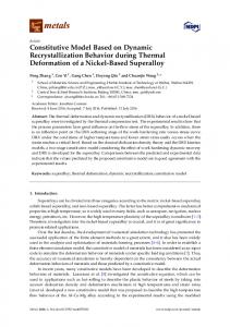
with X∗ = 12 limj→∞ Wj . Here, a reasonable stopping criterion is given by kAj + In k < τ , see (19). If we consider the Lyapunov equations (4) defining the controllability and observability Gramians of stable LTI systems, we observe the following facts which will be of importance for an efficient implementation of (21) in the context of model reduction: 1. The right-hand side is given in factored form, that is, W = BB T or W = C T C, and hence semidefinite. Thus, X is positive semidefinite [LT85], and can therefore also be factored as X = SS T . A possibility here is a Cholesky factorization. 2. Usually, the number of states in (1) is much larger than the number of inputs and outputs, that is, n ≫ m, p. In many cases, this yields a solution matrix with rapidly decaying eigenvalues so that its numerical rank is small; see [ASZ02, Gra04, Pen00] for partial explanations of this fact. Figure 2 demonstrates this behavior for the controllability Gramian of a random stable LTI system with n = 500, m = 10, and stability margin (minimum distance of Λ (A) to R) ≈ 0.055. Hence, if nε is the numerical rank of X, then there is a matrix Sε ∈ Rn×nε so that X ≈ Sε SεT at the level of machine accuracy. Eigenvalues in decreasing order

50

10

eigenvalues machine precision 0

λ

k

10

−50

10

−100

10

−150

10

0

50

100

150

200

250

300

350

400

450

500

k

Figure 2: Eigenvalue decay rate for the controllability Gramian of a random LTI system with n = 500, m = 10, and stability margin ≈ 0.055. The second observation also serves as the basic idea of most algorithms for large-scale Lyapunov equations; see [Pen00, AS01] as well as Chapters [GL05] and [MS05]. Storing Sε is 13

much cheaper than storing X or S as instead of n2 only n · nε real numbers need to be stored. In the example used above to illustrate the eigenvalue decay, this leads already to a reduction factor of about 10 for storing the solution of the controllability Gramian; in Example 3.6 this factor is close to 100 so that 99% of the storage is saved. We will make use of this fact in the method proposed for solving (4). For the derivation of the proposed implementation of the sign function method for computing system Gramians, we will use the Lyapunov equation defining the observability Gramian, AT Y + Y A + C T C = 0. Re-writing the iteration for Wj in (21), we obtain with W0 = C0T C0 := C T C: Wj+1

· ¸T · ¸ ´ 1 ³ 1 Cj Cj −1 2 −T = Wj + γj Aj Wj Aj . = −1 γj Cj A−1 2γj 2γj γj Cj Aj j

Thus, in order to compute a factor R of Y = RT R we can instead directly iterate on the factors: · ¸ 1 Cj . (22) C0 ← C, Cj+1 ← p −1 2γj γj Cj Aj

A problem with this iteration is that the number of columns in Cj doubles in each iteration step so that after j ≥ log2 np steps, the required workspace for Cj becomes even larger than n2 . There are several ways to limit this workspace. The first one, initially suggested in [LA93], works with ·an n × n-matrix, sets C0 to the Cholesky factor of C T C, computes a ¸

QR factorization of

Cj γj Cj A−1 j

in each iteration, and uses its R-factor as next Cj -iterate. A

slightly cheaper version of this is given in [BQ99], where (22) is used as long as j ≤ log2 np and only then starts computing QR factorizations in each step. In both cases, it can be shown that limj→∞ Cj is a Cholesky factor of the solution Y of (20). In order to exploit the second observation from above, in [BQ99] it is suggested to keep the number of rows in Cj less than or equal to the (numerical) rank of Y by computing in each iteration step a rank-revealing QR factorization " # · ¸ Rj+1 Tj+1 1 Cj p Πj+1 , (23) = Uj+1 −1 2γj γj Cj Aj 0 Sj+1 where Rj+1 ∈

Rpj+1 ×pj+1

is nonsingular, pj+1 = rank

µ·

Cj γj Cj A−1 j

¸¶

, and kSj+1 k2 is “small

enough” (with respect to a given tolerance threshold for determining the numerical rank) to safely set Sj+1 = 0. Then, the next iterate becomes Cj+1 ← [ Rj+1 Tj+1 ]Πj+1 ,

(24)

and √12 limj→∞ Cj is a (numerical) full-rank factor of the solution Y of (20). The criterion that will be used to select the tolerance threshold for kSj+1 k2 is based on the following considerations. Let " # M1 M2 £ ¤ ˜ = M1 M2 M= , M E1 E2 14

˜ TM ˜ are approximations to a positive semidefinite matrix K ∈ Rn×n . so that M T M and M Assume √ kEj k2 ≤ εkM k2 , j = 1, 2, for some 0 < ε < 1. Then K − MT M

= K− = K−

"

M1T

E1T

M2T

E2T "

˜ TM ˜ M

−

#"

M1 M2 E1

E2

E1T E1 E1T E2 E2T E1 E2T E2

#

#

If M is a reasonable approximation with kM k22 ≈ kKk2 , then the relative error of the two approximations satisfies ˜ TM ˜ k2 < kK − M T M k2 kK − M + O(ε). ≈ kKk2 kKk2

(25)

If ε ∼ u, where u is the machine precision, this shows that neglecting the blocks E1 , E2 in the factor of the approximation to K yields a relative error of size O(u) which is negligible in the presence of roundoff errors. Therefore, in our calculations we choose the numerical rank √ with respect to ε = u. Example 3.7 For the same random LTI system as used in the illustration of the eigenvalue decay in Figure 2, we computed a numerical full-rank factor of the controllability Gramian. The computed rank is 31, and 10 iterations are needed to achieve convergence in the sign function based iteration. Figure 3 shows the development of pj = rank (Cj ) during the iteration. Comparing (24) with the currently best available implementation of Hammarling’s 40 35 30

rank(Cj)

25 20 15 10 5 0

0

2

4

6

8

10

iteration number (j)

Figure 3: Example 3.7, number of columns in Cj in the full-rank iteration composed of (22), (23), and (24). method [Ham82] for computing the Cholesky factor of the solution of a Lyapunov equation, contained in the SLICOT library [BMS+ 99], we note that the sign function-based method (pure Matlab code) required 4.69 sec. while the SLICOT function (compiled and optimized 15

Algorithm 1 Coupled Newton Iteration for Dual Lyapunov Equations. INPUT: Realization (A, B, C) ∈ Rn×n × Rn×m × Rp×n of an LTI system, tolerances τ1 for convergence of (21) and τ2 for rank detection. OUTPUT: Numerical full-rank factors of the controllability and observability Gramians of the LTI system such that Wc = S T S, Wo = RT R. 1: while kA + In k1 > τ1 do −1 2: Use the LU q decomposition or the Gauß-Jordan elimination to compute A . 3:

4:

kAkF and Z := γA−1 . Set γ := kA −1 k F Compute a rank-revealing LQ factorization

¤ 1 £ √ B ZB =: Π 2γ

5: 6:

τ2 k √12γ

7: 9: 10:

L

0

T

S

#

Q

£ ¤ with kSk2 ≤ τ2 k √12γ B ZB k2 . · ¸ R Set B := Π . T Compute a rank-revealing QR factorization 1 √ 2γ

8:

"

·

with kSk2 ≤ £ ¤ Set C := Π R T . Set A := 21 ( γ1 A + Z). end while Set S := B T , R := C.

C CZ

¸

·

C CZ

¸

=: Q

"

R T 0

S

#

Π

k2 .

Fortran 77 code, called via a mex file from Matlab) needed 7.75 sec., both computed using Matlab 7.0.1 on a Intel Pentium M processor at 1.4 GHz with 512 MBytes of RAM. The computed relative residuals kAX + XAT + BB T kF 2kAkF kXkF + kBB T kF

are comparable, 4.6 · 10−17 for the sign function method and 3.1 · 10−17 for Hammarling’s method.

It is already observed in [LL96] that the two sign function iterations needed to solve both equations in (4) can be coupled as they contain essentially the same iteration for the Aj -matrices (the iterates are transposes of each other), hence only one of them is needed. This was generalized and combined with the full-rank iteration (24) in [BCQ98, BQQ00a]. The resulting sign function-based ”spectral projection method” for computing (numerical) full-rank factors of the controllability and observability Gramians of the LTI system (1) is summarized in Algorithm 1.

16

Algorithm 2 Sign Function-based Spectral Projection Method for Block-Diagonalization. INPUT: Z ∈ Rn×n with Λ (Z) ∩ R = ∅. OUTPUT: U ∈ Rn×n nonsingular such that " # Z 11 U −1 ZU = , Λ (Z11 ) = Λ (Z) ∩ C− , Λ (Z22 ) = Λ (Z) ∩ C+ . Z22 Compute sign (Z) using (13). 2: Compute a rank-revealing QR factorization

1:

In − sign (Z) =: U RΠ. 3:

Block-triangularize A as in (12); that is, set T

Z := U ZU =:

"

Z11 Z12 0

Z22

#

.

Solve the Sylvester equation Z11 Y − Y Z22 + Z12 = 0 using (18). {Note: Z11 , −Z22 are stable!} 5: Set " #" #" # " # Ik −Y Z11 Z12 Ik Y Z11 Z := = , 0 In−k 0 In−k 0 Z22 Z22

4:

3.4

U := U

"

Ik

Y

0

In−k

#

Block-Diagonalization

In the last section we used the block-diagonalization properties of the sign function method to derive an algorithm for solving linear matrix equations. This feature will also turn out to be useful for other problems such as modal truncation and model reduction of unstable systems. The important equation in this context is (17), which allows us to eliminate the off-diagonal block of a block-triangular matrix by solving a Sylvester equation. A spectral projection method for the block-diagonalization of a matrix Z having no eigenvalues on the imaginary axis is summarized in Algorithm 2. In case of purely imaginary eigenvalues, it can still be used if applied to Z + αIn , where α ∈ R is an appropriate spectral shift which is not the real part of an eigenvalue of Z. Note that the computed transformation matrix is not orthogonal, but its first n columns are orthonormal.

4 4.1

Model Reduction Using Spectral Projection Methods Modal Truncation

Modal truncation is probably one of the oldest model reduction techniques [Dav66, Mar66]. In some engineering disciplines, modified versions are still in use, mainly in structural dynamics. In particular, the model reduction method in [CB68] and its relatives, called nowadays substructuring methods, which combine the modal analysis with a static compensation following Guyan [Guy68], are frequently used. We will not elaborate on these type of methods, but 17

.

will only focus on the basic principles of modal truncation and how it can be implemented using spectral projection ideas. The basic idea of modal truncation is to project the dynamics of the LTI system (1) onto an A-invariant subspace corresponding to the dominant modes of the system (poles of G(s), eigenvalues of A that are not canceled by zeros). In structural dynamics software as ANSYS [ANS] or Nastran [MSC], usually an eigenvector basis of the chosen modal subspace is used. Employing the block-diagonalization abilities of the sign function method described in Subsection 3.4, it is easy to derive a spectral projection method for modal truncation. This was first observed by Roberts in his original paper on the matrix sign function [Rob80]. It has the advantage that we avoid a possible ill-conditioning in the eigenvector basis. An obvious, though certainly not always optimal, choice of dominant modes is to select those eigenvalues of A having nonnegative or small negative real parts. Basically, these eigenvalues dominate the long-term dynamics of the solution of the linear ordinary differential equation describing the dynamics of (1)—solution components corresponding to large negative real parts decay rapidly and mostly play a less important (negligible) role in vibration analysis or control design. This viewpoint is rather naive as it neither takes into account the transient behavior of the dynamical system nor the oscillations caused by large imaginary parts or the sensitivity of the eigenvalues with respect to small perturbations. Nevertheless, this approach is often successful when A comes from an FEM analysis of an elliptic operator such as those arising in linear elasticity or heat transfer processes. An advantage of modal truncation is that the poles of the reduced-order system are also poles of the original system. This is important in applications such as vibration analysis since the modes correspond to the resonance frequencies of the original system; the most important resonances are thus retained in the reduced-order model. In the sequel we will use the naive mode selection criterion described above in order to derive a simple implementation of modal truncation employing a spectral projector. The approach, essentially already contained in the original work by Roberts [Rob80], is based on selecting a stability margin α > 0, which determines the maximum modulus of the real parts of the modes to be preserved in the reduced-order model. Now, the eigenvalues of A+αIn are the eigenvalues of A, shifted by α to the right. That is, all eigenvalues with stability margin less than α become unstable eigenvalues of A + αIn . Then, applying the sign function to A + αIn yields the spectral projector 12 (In + sign (A + αIn )) onto the unstable invariant subspace of A+αIn which equals the A-invariant subspace corresponding to the modes that are dominant with respect to the given stability margin. Block-triangularization of A using (12), followed by block-diagonalization based on (17) give rise to the modal truncation implementation outlined in Algorithm 3. In principle, Algorithm 2 could also be used here, but the variant in Algorithm 3 is adapted to the needs of modal truncation and slightly cheaper. The error of modal truncation can easily be quantified. It follows immediately that ˆ G(s) − G(s) = C2 (sI − A22 )−1 B2 ; see also (42) below or [GL95, Lemma 9.2.1]. As A22 , B2 , C2 are readily available, the L2 error for the outputs or H∞ -error for the transfer function (see (10)) is computable. For diagonalizable A22 , we obtain the upper bound ˆ ∞ ≤ cond2 (T ) kC2 k2 kB2 k2 kG − Gk

18

1 minλ∈Λ (A22 ) |Re(λ)|

,

(26)

Algorithm 3 Spectral Projection Method for Modal Truncation. INPUT: Realization (A, B, C, D) ∈ Rn×n × Rn×m × Rp×n × Rp×m of an LTI system (1); a stability margin α > 0, α 6= Re(λ) for all λ ∈ Λ (A). ˆ B, ˆ C, ˆ D) ˆ of a reduced-order model. OUTPUT: Realization (A, 1: Compute S := sign (A + αIn ). 2: Compute a rank-revealing QR factorization S =: QRΠ. 3: Compute (see (12)) " # · ¸ · ¸ A11 A12 B1 C1 T T Q AQ =: , Q B =: , CQ =: . B2 C2 0 A22 4:

Solve the Sylvester equation (A11 − βIk )Y − Y (A22 − βIk ) + A12 = 0 using (18). {Note: If A is stable, β = 0 can be chosen; otherwise set β≥

max

λ∈Λ (A11 )∩C+

(Re(λ)),

e.g., β = 2kA11 kF .} 5: The reduced-order model is then Aˆ := A11 ,

ˆ := B1 − Y B2 , B

Cˆ := C1 ,

ˆ := D. D

where T −1 A22 T = D is the spectral decomposition of A22 and cond2 (T ) is the spectral norm condition number of its eigenvector matrix T . As mentioned at the beginning of this section, several extensions and modifications of modal truncation are possible. In particular, static compensation can account for the steadystate error inherent in the reduced-order model; see, e.g., [F¨ol94] for an elaborate variant. This is related to singular perturbation approximation; see also subsection 4.3 below.

4.2

Balanced Truncation

The basic idea of balanced truncation is to compute a balanced realization µ· ¸ · ¸ ¶ £ ¤ A11 A12 B1 (T AT −1 , T B, CT −1 , D) = , , C1 C2 , D , A21 A22 B2

(27)

where A11 ∈ Rr×r , B1 ∈ Rr×m , C1 ∈ Rp×r , with r less than the McMillan degree n ˆ of the system, and then to use as the reduced-order model the truncated realization ˆ B, ˆ C, ˆ D) ˆ = (A11 , B1 , C1 , D). (A,

(28)

This idea dates essentially back to [Moo81, MR76]. Collecting results from [Moo81, Glo84, TP87], the following result summarizes the properties of balanced truncation. Proposition 4.1 Let (A, B, C, D) be a realization of a stable LTI system with McMillan ˆ B, ˆ C, ˆ D) ˆ with associated transfer function G ˆ degree n ˆ and transfer function G(s) and let (A, be computed as in (27)–(28). Then the following holds:

19

ˆ is balanced, minimal, and stable. Its Gramians are a) The reduced-order system G   σ1  .. ˆ=Σ ˆ = Pˆ = Q  . . σr b) The absolute error bound ˆ ∞≤2 kG − Gk

n ˆ X

σk .

(29)

k=r+1

holds.

ˆ c) If r = n ˆ , then (28) is a minimal realization of G and G = G. Of particular importance is the error bound (29) as it allows an adaptive choice of the order of the reduced-order model based on a prescribed tolerance threshold for the approximation quality. (The error bound (29) can be improved in the presence of Hankel singular values with multiplicity greater than one—they need to appear only once in the sum on the right-hand side.) It is easy to check that for a controllable and observable (minimal) system, i.e., a system with nonsingular Gramians, the matrix 1

T = Σ 2 U T R−T

(30)

provides a balancing state-space transformation. Here Wc = RT R and RWo RT = U Σ2 U T is a singular value decomposition. A nice observation in [LHPW87, TP87] allows us to compute (28) also for non-minimal systems without the need to compute the full matrix T . The first part of this observation is that for Wo = S T S, S −T (Wc Wo )S T = (SRT )(SRT )T = (U ΣV T )(V ΣU T ) = U Σ2 U T so that U, Σ can be computed from an SVD of SRT , · ¸· T ¸ £ ¤ Σ1 0 V1 T SR = U1 U2 , 0 Σ2 V2T

Σ1 = diag(σ1 , . . . , σr ).

(31)

The second part needed is the fact that computing −1/2

Tl = Σ1 and

V1T R,

Aˆ := Tl ATr ,

−1/2

Tr = S T U1 Σ1

ˆ := Tl B, B

,

(32)

Cˆ := CTr

(33)

is equivalent to first computing a minimal realization of (1), then balancing the system as in (27) with T as in (30), and finally truncating the balanced realization as in (28). In particular, the realizations obtained in (28) and (33) are the same, Tl contains the first r rows of T and Tr the first r columns of T −1 —those parts of T needed to compute A11 , B1 , C1 in (27). Also note that the product Tr Tl is a projector onto an r-dimensional subspace of the state-space and model reduction via (33) can therefore be seen as projecting the dynamics of the system onto this subspace. 20

Algorithm 4 Spectral Projection Method for Balanced Truncation. INPUT: Realization (A, B, C, D) ∈ Rn×n × Rn×m × Rp×n × Rp×m of an LTI system (1); a tolerance τ for the absolute approximation error or the order r of the reduced-order model. OUTPUT: Stable reduced-order model, error bound δ. 1: Compute full-rank factors S,R of the system Gramians using Algorithm 1. 2: Compute the SVD " #· ¸ £ ¤ Σ1 V1T T SR =: U1 U2 , V2T Σ2

such that Σ1 ∈ Rr×r is diagonal with the r largest Hankel singular values in decreasing order on its diagonal. HereP r is either the fixed order provided on input or chosen as ˆ minimal integer such that 2 nj=r+1 σj ≤ τ . −1/2

−1/2

Set Tl := Σ1 V1T R, Tr = S T U1 Σ1 4: Compute the reduced-order model, 3:

.

ˆ := Tl B, Aˆ := Tl ATr , B Pˆ and the error bound δ := 2 nj=r+1 σj .

Cˆ := CTr ,

ˆ := D, D

The algorithm resulting from (33) is often referred to as the SR method for balanced truncation. In [LHPW87, TP87] and all textbooks treating balanced truncation, S and R are assumed to be the (square, triangular) Cholesky factors of the system Gramians. In [BQQ00a] it is shown that everything derived so far remains true if full-rank factors of the system Gramians are used instead of Cholesky factors. This yields a much more efficient implementation of balanced truncation whenever n ˆ ≪ n (numerically). Low numerical rank of the Gramians usually signifies a rapid decay of their eigenvalues, as shown in Figure 3, and implies a rapid decay of the Hankel singular values. The resulting algorithm, derived in [BQQ00a], is summarized in Algorithm 4. It is often stated that balanced truncation is not suitable for large-scale problems as it requires the solution of two Lyapunov equations, followed by an SVD, and that both steps require O(n2 ) storage and O(n3 ) flops. This is not true for Algorithm 4 although it does not completely break the O(n2 ) storage and O(n3 ) flops barriers. In Subsection 5.2 it will be shown that by reducing the complexity of the first stage of Algorithm 4 down to O(n·q(log n)), where q is a quadratic or cubic polynomial, it is possible to break this curse of dimensionality for certain problem classes. An analysis of Algorithm 4 reveals the following: assume that A is a full matrix with no further structure to be exploited, and define nco := max{rank (S) , rank (R)} ≪ n, where by abuse of notation “rank” denotes the numerical rank of the factors of the Gramians. Then the storage requirements and computational cost are as follows: 1. The solution of the dual Lyapunov equations splits into three separate iterations: (a) The iteration for Aj requires the inversion of a full matrix and thus needs O(n2 ) storage and O(n3 ) flops. 21

(b) The iterations for Bj and Cj need an additional O(n · nco ) storage, all computations can be performed in O(n2 nco ) flops. The n2 part in the complexity comes from applying A−1 j using either forward and backward substitution or matrix multiplication—if this can be achieved in a cheaper way as in Subsection 5.2, the complexity reduces to O(n · n2co ). 2. Computing the SVD of SRT only needs O(n2co ) workspace and O(n · nco ) flops and therefore does not contribute significantly to the cost of the algorithm. 3. The computation of the ROM via (32) and (33) requires O(r2 ) additional workspace and O(nnco r + n2 r) flops where the n2 part corresponds to the cost of matrix-vector multiplication with A and is not present if this is cheaper than the usual 2n2 flops. An even more detailed analysis shows that the implementation of the SR method of balanced truncation outlined in Algorithm 4 can be significantly faster than the one using Hammarling’s method for computing Cholesky factors of the Gramians as used in SLICOT [BMS+ 99, Var01] and Matlab; see [BQQ00a]. It is important to remember that if A has a structure that allows to store A in less than O(n2 ), to solve linear systems in less than O(n3 ) and to do matrixvector multiplication in less than O(n2 ), the complexity of Algorithm 4 is less than O(n2 ) in storage and O(n3 ) in computing time! If the original system is highly unbalanced (and hence, the state-space transformation matrix T in (27) is ill-conditioned), the balancing-free square-root (BFSR) balanced truncation algorithm suggested in [Var91] may provide a more accurate reduced-order model in the presence of rounding errors. It combines the SR implementation from [LHPW87, TP87] with the balancing-free model reduction approach in [SC89]. The BFSR algorithm only differs from the SR implementation in the procedure to obtain Tl and Tr from the SVD (31) of SRT , and in that the reduced-order model is not balanced. The main idea is that in order to compute the reduced-order model it is sufficient to use orthogonal bases for range (Tl ) and range (Tr ). These can be obtained from the following two QR factorizations: ¸ · · ¸ ¯ ˆ R R , RT V1 = [Q1 Q2 ] S T U1 = [P1 P2 ] , (34) 0 0 ˆ R ¯ ∈ Rr×r are upper triangular. The where P1 , Q1 ∈ Rn×r have orthonormal columns, and R, reduced-order system is then given by (33) with Tl = (QT1 P1 )−1 QT1 ,

Tr = P1 ,

(35)

where the (QT1 P1 )−1 factor is needed to preserve the projector property of Tr Tl . The absolute error of a realization of order r computed by the BFSR implementation of balanced truncation satisfies the same upper bound (29) as the reduced-order model computed by the SR version. 4.2.1

Numerical Experiments

We compare modal truncation, implemented as Matlab function modaltrunc following Algorithm 3 and balanced truncation, implemented as Matlab function btsr following Algorithm 4 for some of the benchmark examples presented in Part II of this book. The Matlab codes are available from 22

http://www.tu-chemnitz.de/∼benner/software.php In the comparison we included several Matlab implementations of balanced truncation based on using the Bartels-Stewart or Hammarling’s method for computing the system Gramians: – the SLICOT [BMS+ 99] implementation of balanced truncation, called via a mex-function from the Matlab function bta [Var01], – the Matlab Control Toolbox (Version 6.1 (R14SP1)) function balreal followed by modred, – the Matlab Robust Control Toolbox (Version 3.0 (R14SP1)) function balmr. The examples that we chose to compare the methods are: ex-rand This is Example 3.7 from above. rail1357 This is the steel cooling example described in Chapter [BS05]. Here, we chose the smallest of the provided test sets with n = 1357. filter2D This is the optical tunable filter example described in Chapter [HBZ05]. For the comparison, we chose the 2D problem — the 3D problem is well beyond the scope of the discussed implementations of modal or balanced truncation. iss-II This is a model of the extended service module of the International Space Station, for details see Chapter [CV05]. (For a more complete comparison of balanced truncation based on Algorithm 4 and the SLICOT model reduction routines see [BQQ03b].) The frequency response errors for the chosen examples are shown in Figure 4. For the implementations of balanced truncation, we only plotted the error curve for btsr as the graphs produced by the other implementations are not distinguishable with the exception of filter2D where the Robust Control Toolbox function yields a somewhat bigger error for high frequencies (still satisfying the error bound (29)). Note that the frequency response error here is measured as the pointwise absolute error ³ ´ ˆ ˆ kG(jω) − G(jω)k 2 = σmax G(jω) − G(jω) ,

where k.k2 is the spectral norm (matrix 2-norm). From Figure 4 it is obvious that for equal order of the reduced-order model, modal truncation usually gives a much worse approximation than balanced truncation. Note that the order r of the reduced-order models was selected based on the reduced-order model computed via Algorithm 3 for a specific, problem-dependent stability margin α. We chose α = 244 for ex-rand, α = 0.01 for rail1357, α = 5 · 103 for filter2D, and α = 0.005 for iss-II. That is, the reduced-order models computed by balanced truncation used a fixed order rather than an adaptive selection of the order based on (29). The computation times obtained using Matlab 7.0.1 on a Intel Pentium M processor at 1.4 GHz with 512 MBytes of RAM are given in Table 1. Some peculiarities we found in the results:

23

Random example: n=500, m=p=10, r=12.

0

Rail cooling: n=1357, m=7, p=6, r=65

0

10

10

BT error bound modal truncation balanced truncation

−2

10 −2

σmax( G(jω) − G65(jω) )

σmax(G(jω) − Gr(jω) )

10

−4

10

−6

10

−4

10

−6

10

−8

10

−10

10

−8

10

modal truncation BT error bound balanced truncation

−10

10

−2

10

0

−12

10

−14

2

10

10

4

10

10

6

−2

10

10

0

10

4

10

6

10

Frequency(ω)

Optical tunable filter (2D): n=1668, m=1, p=5, r=21.

2

2

10

Frequency (ω)

ISS−II: n=1412, m=p=3, r=66

0

10

10

0 −2

10

σmax ( G(jω) − G66(jω) )

σmax( G(jω) − G21(jω) )

10

−2

10

BT error bound modal truncation balanced truncation BT − RC Toolbox

−4

10

−6

10

−4

10

−6

10

−8

10

−8

10

−10

10

modal truncation BT error bound balanced truncation

−10

−2

10

0

10

2

10

4

10

10

6

10

−2

10

Frequency (ω)

0

10

2

10

4

10

6

10

Frequency (ω)

Figure 4: Frequency response (pointwise absolute) error for the Examples ex-rand, rail1357, filter2D, iss-II. – the error bound (29) for ex-rand as computed by the Robust Control Toolbox function is 2.2·10−2 ; this compares unfavorably to the correct bound 4.9·10−5 , returned correctly by the other implementations of balanced truncation. Similarly, for filter2D, the Robust Control Toolbox function computes an error bound 10, 000 times larger than the other routines and the actual error. This suggests that the smaller Hankel singular values computed by balmr are very incorrect. – The behavior for the first 3 examples regarding computing time is very much consistent while the iss-II example differs significantly. The reason is that the sign function does converge very slowly for this particular example and the full-rank factorization computed reveals a very high numerical rank of the Gramians (roughly n/2). This results in fairly expensive QR factorizations at later stages of the iteration in Algorithm 1. Altogether, spectral projection-based balanced truncation is a viable alternative to other balanced truncation implementations in Matlab. If the Gramians have low numerical rank, the execution times are generally much smaller than for approaches based on solving the Lyapunov equations (4) employing Hammarling’s method. On the other hand, Algorithm 4 suffers much from a high numerical rank of the Gramians due to high execution times of Algorithm 1 in that case. The accuracy of all implementations is basically the same for all investigated examples—an observation in accordance to the tests reported in [BQQ00a, BQQ03b]. Moreover, the efficiency of Algorithm 4 allows an easy and highly scalable parallel 24

Example ex-rand rail1357 filter2D iss-II

Modal Trunc. Alg. 3 11.36 203.80 353.27 399.65

Alg. 4 5.35 101.78 152.85 1402.13

Balanced Truncation SLICOT balreal/modred 14.24 21.44 241.44 370.56 567.46 351.26 247.21 683.72

balmr 34.78 633.25 953.54 421.69

Table 1: CPU times needed in the comparison of modal truncation and different balanced truncation implementations for the chosen examples. implementation in contrast to versions based on Hammarling’s method, see Subsection 5.1. Thus, much larger problems can be tackled using a spectral projection-based approach.

4.3 4.3.1

Balancing-Related Methods Singular Perturbation Approximation

In some situations, a reduced-order model with perfect matching of the transfer function at s = 0 is desired. In technical terms, this means that the DC gain is perfectly reproduced. In statespace, this can be interpreted as zero steady-state error. In general this can not be achieved by balanced truncation which performs particularly well at high frequencies (ω → ∞), with a perfect match at ω = ∞. However, DC gain preservation is achieved by singular perturbation ˜ B, ˜ C, ˜ D) denote a minimal realization approximation (SPA), which proceeds as follows: let (A, of the LTI system (1), and partition " # · ¸ A11 A12 B1 ˜ ˜ A= , B= , C˜ = [ C1 C2 ], B2 A21 A22 according to the desired size r of the reduced-order model, that is, A11 ∈ Rr×r , B1 ∈ Rr×m , and C1 ∈ Rp×r . Then the SPA reduced-order model is obtained by the following formulae [LA86]: ˆ := B1 + A12 A−1 B2 , Aˆ := A11 + A12 A−1 B 22 A21 , 22 (36) −1 ˆ := D + C2 A−1 B2 . Cˆ := C1 + C2 A22 A21 , D 22 The resulting reduced-order model satisfies the absolute error bound in (29). When computing the minimal realization with Algorithm 4 or its balancing-free variant, followed by (36), we can consider the resulting model reduction algorithm as a spectral projection method for SPA. Further details regarding the parallelization of this implementation of SPA, together with several numerical examples demonstrating its performance, can be found in [BQQ00b]. 4.3.2

Cross-Gramian Methods

In some situations, the product Wc Wo of the system Gramians is the square root of the solution of the Sylvester equation AWco + Wco A + BC = 0.

(37)

The solution Wco of (37) is called the cross-Gramian of the system (1). Of course, for (37) 2 = W W if to be well-defined, the system must be square, i.e., p = m. Then we have Wco c o 25

• the system is symmetric, which is trivially the case if A = AT and C = B T (in that case, both equations in (4) equal (37)) [FN84a]; • the system is a single-input/single-output (SISO) system, i.e., p = m = 1 [FN84b]. In both cases, instead of solving (4) it is possible to use (37). Also note that the crossGramian carries information of the LTI system and its internally balanced realization if it is not the product of the controllability and observability Gramian and can still be used for model reduction; see [Ald91, FN84b]. The computation of a reduced-order model from the cross-Gramian is based on computing the dominant Wco -invariant subspace which can again be achieved using (13) and (12) applied to a shifted version of Wco . For p, m ≪ n, a factorized version of (18) can be used to solve (37). This again can reduce significantly both the work space needed for saving the cross-Gramian and the computation time in case Wco is of low numerical rank; for details see [Ben04]. Also note that the Bj iterates in (18) need not be computed as they equal the Aj ’s. This further reduces the computational cost of this approach significantly. 4.3.3

Stochastic Truncation

We assume here that 0 < p ≤ m, rank (D) = p, which implies that G(s) must not be strictly proper. For strictly proper systems, the method can be applied introducing an ǫ-regularization by adding an artificial matrix D = [ǫIp 0] [Glo86]. Balanced stochastic truncation (BST) is a model reduction method based on truncating a balanced stochastic realization. Such a realization is obtained as follows; see [Gre88] for details. Define the power spectrum Φ(s) = G(s)GT (−s), and let W be a square minimum phase right spectral factor of Φ, satisfying Φ(s) = W T (−s)W (s). As D has full row rank, E := DDT is positive definite, and a minimal state-space realization (AW , BW , CW , DW ) of W is given by (see [And67a, And67b]) AW CW

:= A, 1 T X ), := E − 2 (C − BW W

BW DW

:= BDT + Wc C T , 1 := E 2 ,

where Wc = S T S is the controllability Gramian defined in (4), while XW is the observability Gramian of W (s) obtained as the stabilizing solution of the algebraic Riccati equation (ARE) T F T X + XF + XBW E −1 BW X + C T E −1 C = 0,

(38)

with F := A − BW E −1 C. Here, XW is symmetric positive (semi-)definite and thus admits a decomposition XW = RT R. If a reduced-order model is computed from an SVD of SRT as ˆ B, ˆ C, ˆ D) ˆ is stochastically balanced. in balanced truncation, then the reduced-order model (A, ˆ c, X ˆ W of the reduced-order model satisfy That is, the Gramians W ˆ c = diag (σ1 , . . . , σr ) = X ˆW , W

(39)

where 1 = σ1 ≥ σ2 ≥ . . . ≥ σr > 0. The BST reduced-order model satisfies the following relative error bound: n Y 1 + σj σr+1 ≤ k∆r k∞ ≤ − 1, (40) 1 − σj j=r+1

26

ˆ From that we obtain where G∆r = G − G.

n Y ˆ ∞ 1 + σj kG − Gk ≤ − 1. kGk∞ 1 − σj

(41)

j=r+1

Therefore, BST is also a member of the class of relative error methods which aim at minimizing k∆r k for some system norm. Implementing BST based on spectral projection methods differs in several ways from the versions proposed in [SC88, VF93], though they are mathematically equivalent. Specifically, the Lyapunov equation for Wc is solved using the sign function iteration described in subsection 3.3, from which we obtain a full-rank factorization Wc = S T S. The same approach ˜ W to XW is used to compute a full-rank factor R of XW fromh a stabilizing approximation X i ˆ T 0 U be an LQ decomposition of D. using the technique described in [Var99]: let D = D ˆ ∈ Rp×p is a square, nonsingular matrix as D has full row rank. Now set Note that D ˆ −T C, HW := D

ˆW := BW D ˆ −1 , B

T ˆW Cˆ := (HW − B X).

Then the ARE (38) is equivalent to AT X + XA + Cˆ T Cˆ = 0. Using a computed approximation ˜ W of XW to form C, ˆ the Cholesky or full-rank factor R of XW can be computed directly X from the Lyapunov equation A(RT R) + (RT R)A + Cˆ T Cˆ = 0. ˜ W is obtained by solving (38) using Newton’s method with exact line The approximation X search as described in [Ben97] with the sign function method used for solving the Lyapunov equations in each Newton step; see [BQQ01] for details. The Lyapunov equation for R is solved using the sign function iteration from subsection 3.3. 4.3.4

Further Riccati-Based Truncation Methods

There is a variety of other balanced truncation methods for different choices of Gramians to be balanced; see, e.g., [GA03, Obe91]. Important methods are positive-real balancing: here, passivity is preserved in the reduced-order model which is an important task in circuit simulation; bounded-real balancing: preserves the H∞ gain of the system and is therefore useful for robust control design; LQG balancing: a closed-loop model reduction technique that preserves closed-loop performance in an LQG design. In all these methods, the Gramians are solutions of two dual Riccati equations of a similar structure as the stochastic truncation ARE (38). The computation of full-rank factors of the system Gramians can proceed in an analogous manner as in BST, and the subsequent computation of the reduced-order system is analogous to the SR or BFSR method for balanced truncation. Therefore, implementations of these model reduction approaches with the computational approaches described so far can also be considered as spectral projection methods. The parallelization of model reduction based on positive-real balancing is described in [BQQ04b]; numerical results demonstrating the accuracy of the reduced-order models and the parallel performance can also be found there. 27

4.4

Unstable Systems

Model reduction for unstable systems can be performed in several ways. One idea is based on the fact that unstable poles are usually important for the dynamics of the system, hence they should be preserved. This can be achieved via an additive decomposition of the transfer function as G(s) = G− (s) + G+ (s), ˆ − , and with G− (s) stable, G+ (s) unstable, applying balanced truncation to G− to obtain G setting ˆ ˆ − (s) + G+ (s), G(s) := G thereby preserving the unstable part of the system. Such a procedure can be implemented using the spectral projection methods for block-diagonalization and balanced truncation: first, apply Algorithm 2 to A and set # " A 0 11 , A˜ := U −1 AU = 0 A22 · ¸ ˜ := U −1 B =: B1 , C˜ := CU =: [ C1 C2 ] , D ˜ := D. B B2 This yields the desired additive decomposition as follows: G(s)

= = =

˜ ˜ −1 B ˜ +D ˜ C(sI − A)−1 B + D = C(sI − A) " #· ¸ £ ¤ (sIk − A11 )−1 B1 C1 C2 +D B2 (sIn−k − A22 )−1 ª © ª © C1 (sIk − A11 )−1 B1 + D + C2 (sIn−k − A22 )−1 B2

(42)

=: G− (s) + G+ (s).

Then apply Algorithm 4 to G− and obtain the reduced order model by adding the transfer functions of the stable reduced and the unstable unreduced parts as summarized above. This approach is described in more detail in [BCQQ04] where also some numerical examples are given. An extension of this approach using balancing for appropriately defined Gramians of unstable systems is discussed in [ZSW99]. This approach can also be implemented using sign function-based spectral projection techniques similar to the ones used so far. Alternative model reduction techniques for unstable systems based on coprime factorization of the transfer function and application of balanced truncation to the stable coprime factors are surveyed in [Var01]. Of course, the spectral projection-based balanced truncation algorithm described in Section 4.2 could be used for this purpose. The computation of spectral factorizations of transfer functions purely based on spectral projection methods requires further investigation, though.

4.5

Optimal Hankel Norm Approximation

BT and SPA model reduction methods aim at minimizing the H∞ -norm of the error system ˆ However, they usually do not succeed in finding an optimal approximation; see [AA02]. G− G. If a best approximation is desired, a different option is to use the Hankel norm of a stable rational transfer function, defined by kGkH := σ1 (G), 28

(43)

where σ1 (G) is the largest Hankel singular value of G. Note that kGkH is only a semi-norm on the Hardy space H∞ as kGkH = 0 does not imply G ≡ 0. However, semi-norms are often easier to minimize than norms. In particular, using the Hankel norm it is possible to compute a best order-r approximation to a given transfer function in H∞ . It is shown in [Glo84] that ˆ of order r can be computed that minimizes the Hankel a reduced-order transfer function G norm of the approximation error in the following sense: ˆ H = σr+1 ≤ kG − Gk ˜ H kG − Gk ˜ of McMillan degree less than or equal to r. Moreover, there for all stable transfer functions G ˆ That is, we can compute a best are explicit formulae to compute such a realization of G. approximation of the system for a given McMillan degree of the reduced-order model which is usually not possible for other system norms such as the H2 - or H∞ -norms. ˆ is quite involved, see, e.g., [Glo84, ZDG96]. Here, we The derivation of a realization of G only describe the essential computational tools required in an implementation of the HNA method. ˆ B, ˆ C, ˆ D) ˆ of the reduced-order model essentially conThe computation of a realization (A, sists of four steps. In the first step, a balanced minimal realization of G is computed. This can be done using the SR version of the BT method as given in Algorithm 4. Next a transfer function ˜ ˜ ˜ −1 B ˜ +D ˜ G(s) = C(sI − A) with the same McMillan degree as the original system (1) is computed as follows: first, the order r of the reduced-order model is chosen such that the Hankel singular values of G satisfy σ1 ≥ σ2 ≥ . . . ≥ σr > σr+1 = . . . = σr+k > σr+k+1 ≥ . . . ≥ σnˆ > 0, k ≥ 1. Then, by applying appropriate permutations, the minimal balanced realization of G is reordered such that the Gramians become # " ˇ Σ . σr+1 Ik ˇ B, ˇ C, ˇ D ˇ is partitioned according In a third step, the resulting balanced realization given by A, to the partitioning of the Gramians, that is, " # · ¸ A11 A12 B1 ˇ ˇ A= , B= , Cˇ = [ C1 C2 ], B2 A21 A22 where A11 ∈ Rn−k×n−k , B1 ∈ ˜ realization of G: A˜ = ˜ = B C˜ = ˜ = D

Rn−k×m , C1 ∈ Rp×n−k . Then the following formulae define a 2 AT + ΣA ˇ 11 Σ ˇ + σr+1 C T U B T ), Γ−1 (σr+1 1 1 11 ˇ 1 − σr+1 C T U ), Γ−1 (ΣB 1 ˇ − σr+1 U B T , C1 Σ 1 D + σr+1 U.

(44)

ˇ 2 − σ 2 In−k . Here, U := (C2T )† B2 , where M † denotes the pseudoinverse of M , and Γ := Σ r+1 29

˜ such that G(s) ˜ ˜ − (s) + G ˜ + (s) Finally, we compute an additive decomposition of G = G ˜ ˜ where G− is stable and G+ is anti-stable. For this additive decomposition we use exactly ˆ := G ˜ − is an optimal r-th order the same algorithm described in the last subsection. Then G Hankel norm approximation of G. Thus, the main computational tasks of a spectral projection implementation of optimal Hankel norm approximation is a combination of Algorithm 4, the formulae (44), and Algorithm 2; see [BQQ04a] for further details.

5

Application to Large-Scale Systems

5.1

Parallelization

Model reduction algorithms based on spectral projection methods are composed of basic matrix computations such as solving linear systems, matrix products, and QR factorizations. Efficient parallel routines for all these matrix computations are provided in linear algebra libraries for distributed memory computers such as PLAPACK and ScaLAPACK [BCC+ 97, van97]. The use of these libraries enhances both the reliability and portability of the model reduction routines. The performance will depend on the efficiency of the underlying serial and parallel computational linear algebra libraries and the communication routines. Here we will employ the ScaLAPACK parallel library [BCC+ 97]. This is a freely available library that implements parallel versions of many of the kernels in LAPACK [ABB+ 99], using the message-passing paradigm. ScaLAPACK is based on the PBLAS (a parallel version of the serial BLAS) for computation and BLACS for communication. The BLACS can be ported to any (serial and) parallel architecture with an implementation of the MPI or the PVM libraries [GBD+ 94, GLS94]. In ScaLAPACK the computations are performed by a logical grid of np = pr ×pc processes. The processes are mapped onto the physical processors, depending on the available number of these. All data (matrices) have to be distributed among the process grid prior to the invocation of a ScaLAPACK routine. It is the user’s responsibility to perform this data distribution. Specifically, in ScaLAPACK the matrices are partitioned into mb × nb blocks and these blocks are then distributed (and stored) among the processes in column-major order (see [BCC+ 97] for details). Using the kernels in ScaLAPACK, we have implemented a library for model reduction of LTI systems, PLiCMR1 , in Fortran 77. The library contains a few driver routines for model reduction and several computational routines for the solution of related equations in control. The functionality and naming convention of the parallel routines closely follow analogous routines from SLICOT. As part of PLiCMR, three parallel driver routines are provided for absolute error model reduction, two parallel driver routines for relative error model reduction, and an expert driver routine capable of performing any of the previous functions on stable and unstable systems. Table 2 lists all the driver routines. The driver routines are based on several computational routines included in PLiCMR and listed in Table 3. Note that the missing routines in the discrete-time case are available in the Parallel Library in Control (PLiC) [BQQ99], but are not needed in the PLiCMR codes for model reduction of discrete-time systems. 1

Available from http://spine.act.uji.es/∼plicmr.html.

30

Purpose Expert driver SR/BFSR BT alg. SR/BFSR SPA alg. HNA alg. SR/BFSR BST alg. SR/BFSR PRBT alg.

Routine pab09mr pab09ax pab09bx pab09cx pab09hx Continuous-time Discrete-time pab09px –

Table 2: Driver routines in PLiCMR. Purpose Solve dual Lyapunov equations and compute HSV Compute Tl , Tr from SR formulae Compute Tl , Tr from BFSR formulae Obtain reduced-order model from Tl , Tr Spectral division by sign function Factorize TFM into stable/unstable parts ARE solver Sylvester solver Lyapunov solver Lyapunov solver (for the full-rank factor) Dual Lyapunov/Stein solver

Routine pab09ah pab09as pab09aw pab09at pmb05rd ptb01kd Continuous-time Discrete-time pdgecrny – psb04md – pdgeclnw – pdgeclnc – psb03odc psb03odd

Table 3: Computational routines in PLiCMR.

A more detailed introduction to PLiCMR and numerical results showing the model reduction abilities of the implemented methods and their parallel performance can be found in [BQQ03b].

5.2

Data-Sparse Implementation of the Sign Function Method

The key to a balanced truncation implementation based on Algorithm 4 with reduced complexity lies in reducing the complexity of storing A and of performing the required computations with A. Recall that the solution of the Lyapunov equation AT X + XA + C T C = 0

(45)

(or its dual in (4)) with the sign function method (21) involves the inversion, addition and multiplication of n×n matrices. Using an approximation of A in H-matrix format [GH03, GHK03] and formatted H-matrix arithmetic, the complexity of storing A and the aforementioned computations reduces to O(n log2 n). We will briefly describe this approach in the following; for more details and numerical examples see [BB04]. Hierarchical (H-)matrices are a data-sparse approximation of large, dense matrices arising from the discretization of non-local integral operators occurring in the boundary element 31

method or as inverses of FEM discretized elliptic differential operators, but can also be used to represent FEM matrices directly. Important properties of H-matrices are: • only few data are needed for the representation of the matrix, • matrix-vector multiplication can be performed in almost linear complexity (O(n log n)), • sums, products, inverses of H-matrices are of “almost” linear complexity. The basic construction principle of H-matrices can be described as follows: consider matrices over a product index set I × I and partition I × I by an H-tree TI×I , where a problem dependent admissibility condition is used to decide whether a block t × s ⊂ I × I allows for a low rank approximation of this block. Definition 5.1 [GH03] The set of hierarchical matrices is defined by H(TI×I , k) := {M ∈ RI×I | rank (M |t×s ) ≤ k for all

admissible leaves t × s of TI×I }.

Submatrices of M ∈ H(TI×I , k) corresponding to inadmissible leaves are stored as dense blocks whereas those corresponding to admissible leaves are stored in factorized form as rankk matrices, called Rk -format. Figure 5 shows the H-matrix representation with k = 4 of the stiffness matrix of the FEM discretization for a 2D heat equation with distributed control and isolation boundary conditions using linear elements on a uniform mesh, resulting in n = 1024.

Figure 5: H-matrix representation of stiffness matrix for 2D heat equation with distributed control and isolation boundary conditions. Here n = 1024 and k = 4. The formatted arithmetic for H-matrices is not a usual arithmetic as H(TI×I , k) is not a linear subspace of RI×I , hence sums, products, and inverses of H-matrices need to be projected into H(TI×I , k). In short, the operations needed here are 32

Formatted addition (⊕) with complexity NH⊕H = O(nk 2 log n)); the computed H-matrix is the best approximation ( with respect to the Frobenius-norm) in H(TI×I , k) of the sum of two H-matrices. Formatted multiplication (⊙) with complexity NH⊙H = O(nk 2 log2 n); f with complexity N f = O(nk 2 log2 n). Formatted inversion (Inv) H,Inv

For the complexity results, some technical assumptions on the H-tree TI×I are needed. The sign function iteration (21) for (45) using formatted H-matrix arithmetic with AH denoting the H-matrix representation in H(TI×I , k) then becomes A0 ← AH , C0 ← C, for j = 0, 1, 2, . . . ´ 1 ³ f j) , Aj ⊕ γj2 Inv(A Aj+1 ← 2γj i 1 h f C˜j+1 ← √ Cj , γj Cj ⊙ Inv(Aj ) , 2 γj Cj+1 ← R-factor of RRQR as in (24).

(46)

Using this method for solving the Lyapunov equations in the first step of Algorithm 4, we obtain an implementation of balanced truncation requiring only O(nco nk log2 n) storage and O(rnco k 2 n log2 n) flops. Work on this topic is in progress, first numerical results reported in [BB04] are promising that this approach will lend itself to efficient model reduction methods for the control of parabolic partial differential equations.

6

Conclusions and Open Problems

Spectral projection methods, in particular those based on the matrix sign function, provide an easy-to-use and easy-to-implement framework for many model reduction techniques. Using the implementations suggested here, balanced truncation and related methods can easily be applied to systems of order O(103 ) on desktop computers, of order O(104 ) using parallel programming models, and to more or less unlimited orders if sparse implementations based on matrix compression techniques and formatted arithmetic can be used. Further investigations could lead to a combination of spectral projection methods based on the sign function with wavelet techniques for the discretization of partial differential equations. Open problems are the derivation of error bounds for several balancing-related techniques that allow an adaptive choice of the order of the reduced-order model for a given tolerance threshold. This would be particulary important for positive-real balancing as this technique could be very useful in circuit simulation and microsystem technology. The extension of the Riccati-based truncation techniques related to stochastic, positive-real, bounded-real, and LQG balancing to descriptor systems is another topic for further investigations, both theoretically and computationally.

Acknowledgements We would like to thank our co-workers Ulrike Baur, Maribel Castillo, Jos´e M. Claver, Rafa Mayo, and Gregorio Quintana-Ort´ı— only through our collaboration all the results discussed 33

in this work could be achieved. We also gratefully acknowledge the helpful remarks and suggestions of an anonymous referee which significantly improved the presentation of this paper. This work was partially supported by the CICYT project No. TIC2002-004400-C03-01 and project No. P1B-2004-6 of the Fundaci´ on Caixa-Castell´ on/Bancaixa and UJI.

References [AA02]

Antoulas, A.C., Astolfi, A.: H∞ -norm approximation. In: Blondel, V.D., Megretski, A. (editors), 2002 MTNS Problem Book, Open Problems on the Mathematical Theory of Networks and Systems, pages 73–76 (2002). Available online from http://www.nd.edu/~mtns/OPMTNS.pdf.

[ABB+ 99]

Anderson, E., Bai, Z., Bischof, C., Demmel, J., Dongarra, J., Du Croz, J., Greenbaum, A., Hammarling, S., McKenney, A., Sorensen, D.: LAPACK Users’ Guide, SIAM, Philadelphia, PA, third edition (1999).

[Ald91]

Aldhaheri, R.W.: Model order reduction via real Schur-form decomposition. Internat. J. Control, 53:3, 709–716 (1991).

[And67a]

Anderson, B.D.O.: An algebraic solution to the spectral factorization problem. IEEE Trans. Automat. Control, AC-12, 410–414 (1967).

[And67b]

Anderson, B.D.O.: A system theory criterion for positive real matrices. SIAM J. Cont., 5, 171–182 (1967).

[ANS]

ANSYS, Inc., http://www.ansys.com. ANSYS.

[AS01]

Antoulas, A.C., Sorensen, D.C.: Approximation of large-scale dynamical systems, An overview. Int. J. Appl. Math. Comp. Sci., 11:5, 1093–1121 (2001).

[ASZ02]

Antoulas, A.C., Sorensen, D.C., Zhou, Y.: On the decay rate of Hankel singular values and related issues. Sys. Control Lett., 46:5, 323–342 (2002).

[BB04]

Baur, U., Benner, P.: Factorized solution of the Lyapunov equation by using the hierarchical matrix arithmetic. Proc. Appl. Math. Mech., 4:1, 658–659 (2004).

[BCC+ 97]

Blackford, L.S., Choi, J., Cleary, A., D’Azevedo, E., Demmel, J., Dhillon, I., Dongarra, J., Hammarling, S., Henry, G., Petitet, A., Stanley, K., Walker, D., Whaley, R.C.: ScaLAPACK Users’ Guide. SIAM, Philadelphia, PA (1997).

[BCQ98]

Benner, P., Claver, J.M., Quintana-Ort´ı, E.S.: Efficient solution of coupled Lyapunov equations via matrix sign function iteration. In: Dourado, A. et al. (editors), Proc. 3rd Portuguese Conf. on Automatic Control CONTROLO’98, Coimbra, pages 205–210 (1998).

[BCQQ04] Benner, P., Castillo, M., Quintana-Ort´ı, E.S., Quintana-Ort´ı, G.: Parallel model reduction of large-scale unstable systems. In: Joubert, G.R., Nagel, W.E., Peters, F.J., Walter, W.V. (editors), Parallel Computing: Software Technology,

34

Algorithms, Architectures & Applications. Proc. Intl. Conf. ParCo2003, Dresden, Germany, volume 13 of Advances in Parallel Computing, pages 251–258. Elsevier B.V. (North-Holland) (2004). [BD75]

Beavers, A.N., Denman, E.D.: A new solution method for the Lyapunov matrix equations. SIAM J. Appl. Math., 29, 416–421 (1975).

[BD93]

Bai, Z., Demmel, J.: Design of a parallel nonsymmetric eigenroutine toolbox, Part I. In: R.F. Sincovec et al., editor, Proceedings of the Sixth SIAM Conference on Parallel Processing for Scientific Computing, pages 391–398, SIAM, Philadelphia, PA (1993). See also: Tech. Report CSD-92-718, Computer Science Division, University of California, Berkeley, CA 94720.

[BD98]

Bai, Z., Demmel, J.: Using the matrix sign function to compute invariant subspaces. SIAM J. Matrix Anal. Appl., 19:1, 205–225 (1998).

[BDD+ 97]

Bai, Z., Demmel, J., Dongarra, J, Petitet, A., Robinson, H., Stanley, K.: The spectral decomposition of nonsymmetric matrices on distributed memory parallel computers. SIAM J. Sci. Comput., 18, 1446–1461 (1997).

[Ben97]

Benner, P.: Numerical solution of special algebraic Riccati equations via an exact line search method. In: Proc. European Control Conf. ECC 97 (CD-ROM), Paper 786. BELWARE Information Technology, Waterloo, Belgium (1997).

[Ben04]

Benner, P.: Factorized solution of Sylvester equations with applications in control. In: Proc. Intl. Symp. Math. Theory Networks and Syst. MTNS 2004, http://www.mtns2004.be (2004).

[BHM97]

Byers, R., He, C., Mehrmann, V.: The matrix sign function method and the computation of invariant subspaces. SIAM J. Matrix Anal. Appl., 18:3, 615–632 (1997).

[BMS+ 99]

Benner, P., Mehrmann, V., Sima, V., Van Huffel, S., Varga, A.: SLICOT a subroutine library in systems and control theory. In: Datta, B.N. (editor), Applied and Computational Control, Signals, and Circuits, volume 1, chapter 10, pages 499–539. Birkh¨auser, Boston, MA (1999).

[BQ99]

Benner, P., Quintana-Ort´ı, E.S.: Solving stable generalized Lyapunov equations with the matrix sign function. Numer. Algorithms, 20:1, 75–100 (1999).

[BQQ99]

Benner, P., Quintana-Ort´ı, E.S., Quintana-Ort´ı, G.: A portable subroutine library for solving linear control problems on distributed memory computers. In: Cooperman, G., Jessen, E., Michler, G.O. (editors), Workshop on Wide Area Networks and High Performance Computing, Essen (Germany), September 1998, Lecture Notes in Control and Information, pages 61–88. Springer-Verlag, Berlin/Heidelberg, Germany (1999).

[BQQ00a]

Benner, P., Quintana-Ort´ı, E.S., Quintana-Ort´ı, G.: Balanced truncation model reduction of large-scale dense systems on parallel computers. Math. Comput. Model. Dyn. Syst., 6:4, 383–405 (2000).

35

[BQQ00b]

Benner, P., Quintana-Ort´ı, E.S., Quintana-Ort´ı, G.: Singular perturbation approximation of large, dense linear systems. In: Proc. 2000 IEEE Intl. Symp. CACSD, Anchorage, Alaska, USA, September 25–27, 2000, pages 255–260. IEEE Press, Piscataway, NJ (2000).

[BQQ01]

Benner, P., Quintana-Ort´ı, E.S., Quintana-Ort´ı, G.: Efficient numerical algorithms for balanced stochastic truncation. Int. J. Appl. Math. Comp. Sci., 11:5, 1123–1150 (2001).

[BQQ03a]

Benner, P., Quintana-Ort´ı, E.S., Quintana-Ort´ı, G.: Parallel algorithms for model reduction of discrete-time systems. Int. J. Syst. Sci., 34:5, 319–333 (2003).

[BQQ03b]

Benner, P., Quintana-Ort´ı, E.S., Quintana-Ort´ı, G.: State-space truncation methods for parallel model reduction of large-scale systems. Parallel Comput., 29, 1701–1722 (2003).

[BQQ04a]

Benner, P., Quintana-Ort´ı, E.S., Quintana-Ort´ı, G.: Computing optimal Hankel norm approximations of large-scale systems. In: Proc. 43rd IEEE Conf. Decision Contr., pages 3078–3083. Omnipress, Madison, WI (2004).

[BQQ04b]

Benner, P., Quintana-Ort´ı, E.S., Quintana-Ort´ı, G.: Computing passive reducedorder models for circuit simulation. In: Proc. Intl. Conf. Parallel Comp. in Elec. Engrg. PARELEC 2004, pages 146–151. IEEE Computer Society, Los Alamitos, CA (2004).

[BQQ04c]

Benner, P., Quintana-Ort´ı, E.S., Quintana-Ort´ı, G.: Parallel model reduction of large-scale linear descriptor systems via Balanced Truncation. In: High Performance Computing for Computational Science. Proc. 6th Intl. Meeting VECPAR’04, June 28–30, 2004, Valencia, Spain, pages 65–78 (2004).

[BQQ04d]

Benner, P., Quintana-Ort´ı, E.S., Quintana-Ort´ı, G.: Solving linear matrix equations via rational iterative schemes. Technical Report SFB393/04-08, Sonderforschungsbereich 393 Numerische Simulation auf massiv parallelen Rechnern, TU Chemnitz, 09107 Chemnitz, FRG (2004). Available from http: //www.tu-chemnitz.de/sfb393/preprints.html.

[BS05]

Benner, P., Saak, J.: A semi-discretized heat transfer model for optimal cooling of steel profiles. In: Benner, P., Mehrmann, V., Sorensen, D.C. (editors), Dimension Reduction of Large-Scale Systems, vol. 45 of Lecture Notes in Computational Science and Engineering, Springer-Verlag, Berlin/Heidelberg (2005).

[Bye87]

Byers, R.: Solving the algebraic Riccati equation with the matrix sign function. Linear Algebra Appl., 85, 267–279 (1987).

[CB68]

Craig, R.R., Bampton, M.C.C.: Coupling of substructures for dynamic analysis. AIAA J., 6, 1313–1319 (1968).

[CV05]

Chahlaoui, Y., Van Dooren, P.: Benchmark examples for model reduction of linear time-invariant dynamical systems. In: Benner, P., Mehrmann, V., Sorensen, D.C. (editors), Dimension Reduction of Large-Scale Systems, vol. 45 of Lecture Notes in Computational Science and Engineering, Springer-Verlag, Berlin/Heidelberg (2005). 36

[Dav66]

Davison, E.J.: A method for simplifying linear dynamic systems. IEEE Trans. Automat. Control, AC-11, 93–101 (1966).

[DB76]

Denman, E.D., Beavers, A.N.: The matrix sign function and computations in systems. Appl. Math. Comput., 2, 63–94 (1976).

[FN84a]

Fernando, K.V., Nicholson, H.: On a fundamental property of the cross-Gramian matrix. IEEE Trans. Circuits Syst., CAS-31:5, 504–505 (1984).

[FN84b]

Fernando, K.V., Nicholson, H.: On the structure of balanced and other principal representations of linear systems. IEEE Trans. Automat. Control, AC-28:2, 228–231 (1984).

[F¨ol94]

F¨ollinger, O.: Regelungstechnik. H¨ uthig-Verlag, 8. edition (1994).

[GA03]

Gugercin, S., Antoulas, A.C.: A survey of balancing methods for model reduction. In: Proc. European Control Conference ECC 2003, Cambridge, UK (2003). CD Rom.

[GBD+ 94]

Geist, A., Beguelin, A., Dongarra, J., Jiang, W., Manchek, B., Sunderam, V.: PVM: Parallel Virtual Machine – A Users Guide and Tutorial for Network Parallel Computing. MIT Press, Cambridge, MA (1994).

[GH03]

Grasedyck, L., W. Hackbusch, W.: Construction and arithmetics of H-matrices. Computing, 70, 295–334 (2003).

[GHK03]

Grasedyck, L., Hackbusch, W., Khoromskij, B.N.: Solution of large scale algebraic matrix Riccati equations by use of hierarchical matrices. Computing, 70, 121–165 (2003).

[GL95]

Green, M., Limebeer, D.J.N.: Linear Robust Control. Prentice-Hall, Englewood Cliffs, NJ (1995).

[GL05]

Gugercin, S., Li, J.-R.: Smith-type methods for balanced truncation of large sparse systems. In: Benner, P., Mehrmann, V., Sorensen, D.C. (editors), Dimension Reduction of Large-Scale Systems, vol. 45 of Lecture Notes in Computational Science and Engineering, Springer-Verlag, Berlin/Heidelberg (2005).

[Glo84]

Glover, K.: All optimal Hankel-norm approximations of linear multivariable systems and their L∞ norms. Internat. J. Control, 39, 1115–1193 (1984).

[Glo86]

Glover, K.: Multiplicative approximation of linear multivariable systems with L∞ error bounds. In: Proc. American Control Conf., pages 1705–1709 (1986).

[GLS94]

Gropp, W., Lusk, E., Skjellum, A.: Using MPI: Portable Parallel Programming with the Message-Passing Interface. MIT Press, Cambridge, MA (1994).

[Gra04]

Grasedyck, L.: Existence of a low rank or H-matrix approximant to the solution of a Sylvester equation. Numer. Lin. Alg. Appl., 11, 371–389 (2004).

[Gre88]

Green, M.: Balanced stochastic realization. Linear Algebra Appl., 98, 211–247 (1988). 37

[Guy68]

Guyan, R.J.: Reduction of stiffness and mass matrices. AIAA J., 3, 380 (1968).

[GV96]

Golub, G.H., Van Loan, C.F.: Matrix Computations. Johns Hopkins University Press, Baltimore, third edition (1996).

[Ham82]

Hammarling, S.J.: Numerical solution of the stable, non-negative definite Lyapunov equation. IMA J. Numer. Anal., 2, 303–323 (1982).

[HBZ05]

Hohlfeld, D., Bechtold, T., Zappe, H.: Tunable Optical Filter. In: Benner, P., Mehrmann, V., Sorensen, D.C. (editors), Dimension Reduction of Large-Scale Systems, vol. 45 of Lecture Notes in Computational Science and Engineering, Springer-Verlag, Berlin/Heidelberg (2005).

[Hig86]

Higham, N.J.: Computing the polar decomposition—with applications. SIAM J. Sci. Statist. Comput., 7, 1160–1174 (1986).

[HMW77]

Hoskins, W.D., Meek, D.S., Walton, D.J.: The numerical solution of A′ Q+QA = −C. IEEE Trans. Automat. Control, AC-22, 882–883 (1977).

[HQSW00] Huss, S., Quintana-Ort´ı, E.S., Sun, X., Wu, J.: Parallel spectral division using the matrix sign function for the generalized eigenproblem. Int. J. of High Speed Computing, 11:1, 1–14 (2000). [KL92]

Kenney, C., Laub, A.J.:. On scaling Newton’s method for polar decomposition and the matrix sign function. SIAM J. Matrix Anal. Appl., 13, 688–706 (1992).

[KL95]

Kenney, C., Laub, A.J.:. The matrix sign function. IEEE Trans. Automat. Control, 40:8, 1330–1348 (1995).

[KMP01]

Konstantinov, M.M., Mehrmann, V., Petkov, P.Hr.: Perturbation analysis for the Hamiltonian Schur form. SIAM J. Matrix Anal. Appl., 23:2, 387–424 (2001).

[LA86]

Liu, Y., Anderson, B.D.O. : Controller reduction via stable factorization and balancing. Internat. J. Control, 44, 507–531 (1986).

[LA93]

Larin, V.B., Aliev, F.A.: Construction of square root factor for solution of the Lyapunov matrix equation. Sys. Control Lett., 20, 109–112 (1993).

[Lev96]

Levine, W.S. (editor): The Control Handbook. CRC Press (1996).

[LHPW87] Laub, A.J., Heath, M.T., Paige, C.C., Ward, R.C.: Computation of system balancing transformations and other application of simultaneous diagonalization algorithms. IEEE Trans. Automat. Control, 34, 115–122 (1987). [LL96]

Lang, W., Lezius, U.: Numerical realization of the balanced reduction of a control problem. In: H. Neunzert, editor, Progress in Industrial Mathematics at ECMI94, pages 504–512, John Wiley & Sons Ltd and B.G. Teubner, New York and Leipzig (1996).

[LR95]

Lancaster, P., Rodman, L.: The Algebraic Riccati Equation. Oxford University Press, Oxford (1995).

38

[LT85]

Lancaster, P., Tismenetsky, M.: Orlando, 2nd edition (1985).

[Mar66]

Marschall, S.A.: An approximate method for reducing the order of a linear system. Contr. Eng., 10, 642–648 (1966).

[Moo81]

Moore, B.C.: Principal component analysis in linear systems: Controllability, observability, and model reduction. IEEE Trans. Automat. Control, AC-26, 17–32 (1981).

[MR76]

Mullis, C., Roberts, R.A.: Synthesis of minimum roundoff noise fixed point digital filters. IEEE Trans. Circuits and Systems, CAS-23:9, 551–562 (1976).

[MS05]

Mehrmann, V., Stykel, T.: Balanced truncation model reduction for large-scale systems in descriptor form. In: Benner, P., Mehrmann, V., Sorensen, D.C. (editors), Dimension Reduction of Large-Scale Systems, vol. 45 of Lecture Notes in Computational Science and Engineering, Springer-Verlag, Berlin/Heidelberg (2005).

[MSC]

MSC.Software Corporation, http://www.mscsoftware.com. MSC.Nastran.

[Mut99]

Mutambara, A.G.O.: Design and Analysis of Control Systems. CRC Press, Boca Raton, FL (1999).

[OA01]

Obinata, G., Anderson, B.D.O.: Model Reduction for Control System Design. Communications and Control Engineering Series. Springer-Verlag, London, UK (2001).

[Obe91]

Ober, R.: Balanced parametrizations of classes of linear systems. SIAM J. Cont. Optim., 29, 1251–1287 (1991).

[Pen00]

Penzl, T.: A cyclic low rank Smith method for large sparse Lyapunov equations. SIAM J. Sci. Comput., 21:4, 1401–1418 (2000).

[Rob80]

Roberts, J.D.: Linear model reduction and solution of the algebraic Riccati equation by use of the sign function. Internat. J. Control, 32, 677–687 (1980). (Reprint of Technical Report No. TR-13, CUED/B-Control, Cambridge University, Engineering Department (1971).)

[SC88]

Safonov, M.G., Chiang, R.Y.: Model reduction for robust control: A Schur relative error method. Int. J. Adapt. Cont. and Sign. Proc., 2, 259–272 (1988).

[SC89]

Safonov, M.G., Chiang, R.Y.: A Schur method for balanced-truncation model reduction. IEEE Trans. Automat. Control, AC-34, 729–733 (1989).

[Son98]

Sontag, E.D.: Mathematical Control Theory. Springer-Verlag, New York, NY, 2nd edition (1998).

[TP87]

Tombs, M.S., I. Postlethwaite, I.: Truncated balanced realization of a stable non-minimal state-space system. Internat. J. Control, 46:4, 1319–1330 (1987).

[van97]

van de Geijn, R.A.: Using PLAPACK: Parallel Linear Algebra Package. MIT Press, Cambridge, MA (1997). 39

The Theory of Matrices. Academic Press,

[Van00]

Van Dooren,P.: Gramian based model reduction of large-scale dynamical systems. In: D.F. Griffiths G.A. Watson, editors, Numerical Analysis 1999. Proc. 18th Dundee Biennial Conference on Numerical Analysis, pages 231–247, Chapman & Hall/CRC, London, UK (2000).

[Var91]

Varga, A.: Efficient minimal realization procedure based on balancing. In: Prepr. of the IMACS Symp. on Modelling and Control of Technological Systems, volume 2, pages 42–47 (1991).

[Var99]

Varga, A.: Task II.B.1 – selection of software for controller reduction. SLICOT Working Note 1999–18, The Working Group on Software (WGS) (1999). Available from http://www.win.tue.nl/niconet/NIC2/reports.html.

[Var01]

Varga, A.: Model reduction software in the SLICOT library. In: B.N. Datta, editor, Applied and Computational Control, Signals, and Circuits, volume 629 of The Kluwer International Series in Engineering and Computer Science, pages 239–282, Kluwer Academic Publishers, Boston, MA (2001).

[VF93]

Varga, A., Fasol, K.H.: A new square–root balancing–free stochastic truncation model reduction algorithm. In: Prepr. 12th IFAC World Congress, volume 7, pages 153–156, Sydney, Australia (1993).

[ZDG96]

Zhou, K., Doyle, J.C., Glover, K.: Robust and Optimal Control. Prentice-Hall, Upper Saddle River, NJ (1996).

[ZSW99]

Zhou, K., Salomon, G., Wu, E.: Balanced realization and model reduction for unstable systems. Int. J. Robust Nonlinear Control, 9:3, 183–198, (1999).

40