Feb 18, 2010 - process using mixtures of Dirichlet processes (DPM). ... of inhomogeneous Gaussian processes, see for example Lemos and Sansó (2009),.
Modeling and Anomaly Detection for Event Occurrences Following an Inhomogeneous Spatio-Temporal Poisson Process Waley W. J. Liang, Jacob B. Colvin, Bruno Sans´o, and Herbert K. H. Lee University of California, Santa Cruz February 18, 2010 Abstract This paper presents a model that describes spatial variations of the intensity of events that occur at random geographical locations. An inhomogeneous Poisson process is used to model the intensity over a spatial region with multiplicative spatial and temporal covariate effects. Dynamic temporal effects are incorporated into the model allowing changes in the intensity structure over time. Additionally, anomaly detection in the event rates is developed based on exceedance probabilities. The methods are demonstrated on data of major crimes in Cincinnati during 2006.
1
Introduction
We consider the problem of inference for time evolving point patterns. We focus on sequences of inhomogeneous Poisson processes with time-varying intensities using a Bayesian approach, proposing a model-based flexible tool and illustrating its use for anomalies detection. As a motivating example we analyze a dataset of major crimes (those involving serious violence against another person) in Cincinnati during 2006. These are depicted by the blue points in Figure 1. We can see that crimes are more concentrated just above the river (where we refer as the downtown area) than they are at other locations. Even at locations where crimes are sparse, small clusters of occurrences are noticeable. Clearly, there is an inhomogeneous underlying structure for the intensity of crimes over Cincinnati and our task is to design and implement a model to describe such intensity. Since each crime occurs at a specific location over the spatial region, the collection of these occurrences can be described by a spatial point process (PP). In general, a spatial PP is a random collection of events occurring in a spatial region where each event is referenced by the location at which it occurs. For example, the arrival of buses on a street, occurrence of mountain fires, and incidence of diseases can all be described by a spatial PP. Typically, the spatial locations are recorded in longitude, latitude, and elevation, though sometimes only one coordinate is of interest. 1
For concreteness we will we will work with PPs on two-dimensional domains, but the results clearly generalize to other dimensional spaces. Moreover, the crimes shown in Figure 1 occur not only at different locations but also at different times. Hence, we consider a spatial PP indexed by time. In this paper we focus on inhomogeneous Poisson processes, for which specification of the intensity function is required. The intensity function defines the rate of occurrence for the Poisson process. This is assumed to vary smoothly in space and time. We use an innovative convolution of a time-varying discrete gamma process. To reduce the computational burden we use compactly supported kernels for the convolution. The result is a model that is flexible but computationally tractable, is able to realistically capture the space and time evolution of observed data, and is able to incorporate information from covariates. In the next section, we give a brief overview of the basics of spatial-temporal point processes, references to some of the existing inferential procedures, and the properties of a Poisson process. In Section 3, we specify the intensity function of the Poisson process, covariates, and priors for the model parameters. In Section 4, extension to the dynamic model and inference based on Forward Filtering Backward Sampling is revealed. Detection of anomalous events based on exceedance probabilities is developed in Section 5. In Section 6, plotting of the results on the crime data and discussions are given.
39.16 39.14 39.12 39.10
Latitude
39.18
39.20
39.22
Cincinnati Crime Data
−84.65
−84.60
−84.55
−84.50
−84.45
−84.40
Longitude
Figure 1: Major crime locations in Cincinnati in 2006.
2
2
Inhomogeneous spatio-temporal Poisson process
A spatio-temporal point process N is defined as a random measure over a region {S × T }, where S ⊆ Rp and T ⊆ R+ . Each point in the process is referenced by a spatial location s ∈ S and time t ∈ T . In this paper, we focus on developing an inhomogeneous spatio-temporal Poisson process model on a two-dimensional spatial domain. Following the description by Kottas and Sans´o (2007), an inhomogeneous spatial Poisson process is a random countable subset Π of S ⊆ R2 . It has the property that for any finite collection A1 , · · · , Ak of pairwise disjoint subsets of S, the random variables N(A1 ), · · · , N(Ak ), i.e., the number of points Rof Π lying in each Aj , are independent and each follows a Poisson distribution with mean λ(s)ds. Here, λ(·) is the intensity function of the inhomogeneous Poisson process. Denote Aj the observation locations by s1 , · · · , sn ∈ S. The likelihood of λ(·) is L(λ) ∝ exp{−Λ(S)}
n Y
λ(si ) ,
i=1
R
where Λ(S) = S λ(s)ds. This model can be extended to allow the intensity to change over time. Suppose that the data corresponds to T different time intervals. In each time interval t we have an intensity function λ(s, t). Let ti be the time that corresponds to the observation at location si and assume that the intensity is constant within each time interval. The likelihood of this extended model is n n n Z oY Y exp − λ(s, ti )ds λ(si , ti ) . (1) L(λ) ∝ i=1
S
i=1
Covariate information (spatial and/or temporal) can be incorporated into λ(s, t) and their effects can be estimated along with other parameters of λ based on observed data. Ripley (1981, 1988), Diggle (1983, 1985), Guttorp and Thompson (1990); Guttorp (1995), Stoyan, Kendall and Mecke (1995), Stoyan and Stoyan (1995) give details of spatial point process in which stationarity or homogeneity is assumed and inference based on non-parametric methods is the focus. For likelihood-based, including simulation-based, inference (e.g., MCMC methods), see Mφller (1999), Lieshout (2000), Diggle (2003), Mφller and Waagepetersen (2003, 2004), Baddeley, Gregori, Mateu, Stoica and Stoyan (2006), and Waagepetersen and Guan (2009). These recent texts often relax the restrictive assumption of stationarity or homogeneity. For spatial-temporal point processes, the papers by Diggle (2005) and by Jensen, J´onsd´ottir, Schmiegel and Barndorff-Nielsen (2006) provide introductions to the subject and some likelihood-based inference methods. Kottas and Sans´o (2007) propose a Bayesian non-parametric approach to modeling the intensity of an inhomogeneous Poisson process using mixtures of Dirichlet processes (DPM). Taddy (2009) extends the model to consider temporally-varying intensities. The DPM is computationally efficient and offers a lot of flexibility, however it can not be easily adapted to handle covariates without substantial loss of computational efficiency.
3
3
A nonparametric model
Based on the above Poisson process likelihood, we need to specify the intensity function λ(s, t), which depends only on (s, t). In our model, it is decomposed as λ(s, t) = τ λ(s)µ(s)ν(t), where τ is a scalar parameter, τ λ(s) is the baseline intensity, µ(s) is the effect due to spatially varying covariates, and ν(t) is the effect due to temporal covariates. The decomposition assumes that spatial and temporal effects due to covariates have a multiplicative effect on the baseline intensity of the process.
3.1
Specification of the baseline intensity
A flexible and computationally efficient way of specifying spatial processes is given by process convolutions (Higdon, Swall and Kern, 1999; Higdon, 2001). While these are mostly used in the context of inhomogeneous Gaussian processes, see for example Lemos and Sans´o (2009), Lee et al. (2008) have used them to model spatial processes with positive values. Following these ideas λ(s), is specified Z λ(s) = k(s − u|ψ)z(u)du, where z(·) is a gamma process and k(·|ψ) is a kernel function with parameter vector ψ. A discrete approximation can be obtained by considering a grid of regularly spaced background points u1 , · · · , um ∈ S and the intensity can be approximated as λ(s) =
m X j=1
k(s − uj |ψ)z(uj ).
(2)
Assuming that z(uj ) follows a gamma distribution ensures a nonnegative intensity. The use of a convolution as defined Equation (2) within the likelihood in Equation (1) entails a computational problem. In fact computing the likelihood requires the evaluation of n products of sums. To tackle this problem we assume that the kernel k(·) is a function with compact support. More specifically we define kB (s − uj |ψ) k(s − uj |ψ) = Pm , j=1 kB (s − uj |ψ)
where kB (·|ψ) is a bivariate anisotropic B´ezier kernel (Brenning, 2001) function with parameter vector ψ. Denote s = (s1 , s2 ), u = (u1 , u2 ), and ψ = (l1 , l2 , w), the form of the kernel is " # � s − u �2 � s − u �2 w 1 1 2 2 kB (s − u|ψ) = 1 − + 1 √((s −u )/l )2 +((s −u )/l )2 ) ≤ 1� , 1 1 1 2 2 2 l1 l2 where u is the center of the kernel, l1 and l2 are the ranges of the support in the s1 and s2 directions such that the kernel is strictly zero beyond these ranges, 1A is the indicator 4
function of the set A, and w is a parameter that governs the smoothness of the resulting process. A B´ezier kernel has a compact elliptical support, which ensures that z(uj )s are more directly associated to the local crime intensity. Moreover, the effective number of terms in the sum of Equation (2) is substantially smaller than m. For n observations, we let λ = (λ(s1 ), · · · , λ(sn ))′ , z = (z(u1 ), · · · , z(um ))′ , and K a n × m matrix such that Kij = k(si − uj |ψ). Then we have the conditionally linear representation of Equation (2), λ = Kz. Thanks to the use of a B´ezier kernel we can use sparse matrix computations in this expression.
3.2
Specification of covariates
Let X(s) be a vector of spatial covariates, such as topographical features, population density or spatial income distribution, and let F(t) be a vector of temporal covariates, such as seasonal effects, typically given as � 2πt �� � � 2πt � , cos , t ∈ {1, · · · , T }. F′ (t) = sin T T
The spatial and temporal effects on the process intensity are given by µ(s) = exp{X′(s)β}, β ∈ Rp ν(t) = exp{F′ (t)φ}, φ ∈ Rq ,
where p and q denote the number of spatial and temporal covariates, respectively. The full likelihood for λ(s, t) can be written as L(λ) ∝ exp{−τ ΛT Λ0 }τ
n
n Y
µ(si )ν(ti )
m X j=1
i=1
k(si − uj |ψ)z(uj )
where ΛT = Λ0 = ≈
T X
t=1 m X
j=1 m X j=1
exp{F′ (t)φ} z(uj )
Z
S
z(uj )
k(s − uj |ψ) exp{X′(s)β}ds
X s∈S
k(s − uj |ψ) exp{X′ (s)β}∆s .
The above approximation follows from the idea that the observation window can be discretized and the intensity within each grid cell is assumed to be constant. The area of a grid cell is denoted by ∆s. 5
3.3
Bayesian inference
We follow a Bayesian approach to estimate the parameters of the model. To proceed, the following priors are imposed on the parameters: z(uj ) ∼ Γ(Az , Bz ), P (τ ) ∝ τ1 , βv ∼ N(0, σβ2v ) and φl ∼ N(0, σφ2l ), where Az , Bz , σβv , and σφl are constants. The resulting posterior distributions are given in the Appendix. Markov Chain Monte Carlo (MCMC) is used to explore the posterior distributions of these parameters. Specifically, Gibbs sampling is used to obtain samples of τ since its posterior distribution can be obtained in closed form. The MetropolisHastings algorithm is used to obtain posterior samples of z(uj ), βv , and φl with the following proposal distributions: ! h−1 z (u ) a (1 − b ) a b j z z z z z ∗ (uj ) ∼ , Beta , bz 2 2 βv∗ ∼ N(βvh−1 , σβ2v∗ ), φ∗l ∼ N(φh−1 , σφ2∗l ), l
where az , bz , σβv∗ , σφ∗l are constants, and h denotes the MCMC iteration index. The multiplicative beta proposal is implemented to improve the acceptance rate of z(uj ) and it seems to induce a fast convergence of the MCMC.
4 4.1
A Dynamic approach Model specification
The model specified in Section 3 incorporates a multiplicative temporal effect on the intensity of the Poisson process using the function F(t) . This implies that temporal covariates can only re-scale the baseline intensity, but not its shape. In other words, the shape of the intensity at any time strongly depends on the entire data set, with little influence of events occurring at the time being considered. Changes in the shape of the space-time intensity due to time can only be captured using a non-separable model. To this end we modify the baseline intensity by making the convolved gamma process z(uj ) time dependent. Given that the convolving kernel has compact support, we expect that the time evolution of the latent process will be determined mostly by the occurrences of events close to the nodes. To obtain a simple yet flexible model for the time evolution of zt (uj ) we use the methods of West and Harrison (1997) and fit a first-order polynomial DLM for the log of zt (uj ). This will account for smooth time variations in the shape of the intensity. Let yt (uj ) = log(zt (uj )). Then Yt = θ t + vt , θ t = θ t−1 + wt ,
6
where Yt = (yt (u1 ), · · · , yt (um ))′ , θ t = (θt (u1 ), · · · , θt (um ))′ ,
vt ∼ N(0, Vt ), wt ∼ N(0, Wt ) ,
vt and wt are the observational error and evolution error, respectively. More elaborate dynamics that include, for example, seasonalities or additional covariates, can be accounted for by using observational and evolution matrices other than the identity. For the observation error variance we take Vt = σ 2 Im . For the evolution error variance we use a discount factor approach (Section 6.3, West and Harrison (1997)). A discount factor is a parameter, δ ∈ (0, 1] that determines the amount of information loss between consecutive time steps in the evolution equation.
4.2
Model fitting
The model specified in the previous section is fitted using an elaboration of the Monte Carlo method developed for the model of Section 3. The full conditionals for the convolution parameters are modified by noting that � � 1 1 1 √ exp − 2 (log(zt (uj )) − θt (uj ))2 , p(zt (uj )) = zt (uj ) σ 2π 2σ
which leads to the expression
π(zt (uj )| · · · ) ∝ exp{−τ Λ} where Λ=
T X t=1
′
exp{F (t)φ}
m X j=1
m T Y nt X Y t=1 i=1 j=1
zt (uj )
X s∈S
k(si − uj |ψ)zt (uj )p(zt (uj )) ,
k(s − uj |ψ) exp{X′ (s)β}∆s .
Following is a rough sketch of the MCMC procedure at each iteration. 1. Sample zt (uj ) from (20) via the Metropolis-Hasting algorithm. 2. Based on the most recently sampled zt (uj )s, compute Yt and sample θ t using the Forward Filtering Backward Sampling algorithm. 3. Sample all other parameters based on the most recently sampled θ t and treating exp(θ t ) as a sample of the underlying discretized gamma process at time t. 4. Repeat steps 1 through 3 for the next MCMC iteration. The proposed dynamic model can be used for predictions of the intensity at any time given data up to the previous time. For example, if we have data from January to November, we can predict the intensity for December using the one-step ahead forecast distribution. For details, refer to Chapter 4 of West and Harrison (1997). 7
5
Anomaly Detection
The proposed model can be used to detect events which are anomalous relative to either its spatial or temporal structure. Following the general approach of Cressie (1991) for examining residuals, we impose a grid over the spatial domain. We consider the number of events in a grid cell in a particular month to be anomalous if it is much larger than would be expected under the Poisson process model. This expected value could either be from data including the month in question (i.e., finding anomalous residuals) or from predictions (checking if new data match predicted values). We typically focus on one-sided tests because of the nonnegative character of counts. We compute a measure of anomaly via exceedance probabilities (EP) based on the Poisson model. A one sided EP is calculated as P = P r(Nt (s) > λt (s)) , where Nt (s) is the observed crime count over region s at time t and λt (s) is the expected number of crimes at time t over region s as fitted or predicted by the poisson process model. A two-sided EP can be defined analogously. Nt (s) is identified as anomalous if P < α, where α is a pre-specified significance level. Typical values of α include 0.01, 0.05, and 0.1. We define two types of anomalies as follows. • Spatial Anomaly: A spatial anomaly occurs when the number of observations is significantly larger than the expected number of counts in a grid cell for all times. This is caused by changes in the intensity function that are not properly modeled by the kernel grid, where the kernel smoothing estimate of the crime intensity function is unable to account for the nonlinear changes in the underlying crime intensity function. This is an indication that the assumed spatial continuity is not present in the observed data, i.e., a particular grid cell is very unlike its neighbors. Spatial EP’s are calculated as X P r(N(s) > λ(s)) = P r(N(s) > λ(s)|λ) × P r(λ) . λ
• Temporal Anomaly: A temporal anomaly occurs when the observed event count in a grid cell is significantly larger than the expected number at a particular time while other time intervals show no significant divergence from model assumptions. Temporal EP’s are calculated as X Pr(Nt (s) > λt (s)|λt ) × P r(λt) . P r(Nt(s) > λt (s)) = λt
6
Example
We now apply the models to the crime data shown in Figure 1. This dataset is publicly available at http://www.cincinnati-oh.gov/police/pages/-4258-/. We discretize the observation window S using a 20 × 20 grid. The center of each grid cell represents the coordinate 8
of the grid cell and also serves as a background location u of the gamma process. One additional row of u is placed outside the observation window on each side to eliminate edge effects. The covariates being considered are the population density and vacancy rates over the observation window. The spatial covariate vector is constructed as X′ (s) = (x1 (s), x2 (s)) ,
(3)
where x1 (s) represents population density and x2 (s) represents vacancy rate at location s. Vacancy rates can be used as a proxy for the economic health of the neighborhood. The given covariate values vary in different parts of S and they have been pre-processed so that each of the covariates has a fixed value within each grid cell. As we are interested in monthly effects, the temporal covariate vector is constructed as � � 2πt � � 2πt �� F′ (t) = sin , cos , t ∈ {1, · · · , 12} . (4) 12 12
Using the priors defined in Section 3.3, the parameter values are chosen as following. The standard deviation (SD) of the spatial effect prior, σβv , is chosen to be 0.05, for both population density and vacancy rate effects. The posterior mean of the population density effect is estimated to be 4.5%, and that of the vacancy rate effect is estimated to be 6.8%, which seem fairly reasonable. The SD of the multiplicative temporal effect prior, σφl , is chosen to be 0.5 and 4 for the sine and cosine terms, respectively. This ensures that this temporal effect is higher in the middle of the year (when it is warmer and more people are out) than at the beginning and end of year, and when averaged, is around 1. The prior shape and rate parameters, Az and Bz of z(u), are chosen to be 75 and 13000, respectively, to ensure a reasonable posterior mean (around 320) for τ under the assumption that τ represents the monthly baseline counts over the entire spatial domain, and τ λ(s)µ(s) represents the proportion of τ that corresponds to grid s. For the dynamic model, the discount factor δ and √ the observational SD σ are chosen to be 0.95 and 0.5, respectively. They should ideally be treated as unknown parameters and estimated via MCMC. But after trying different values of δ within [0.9, 1] (this is the range of values in which a discount factor almost always takes), model results stayed about the same. So, for the purpose of a simpler model, we decided to use the median value, 0.95. The value of σ is chosen to retain the same general structure in the intensity across all months while allowing some shape changes without significantly affecting the convergence of the spatial and temporal effects parameters. The proposal distribution parameters are chosen as az = 2, bz = 0.5, σβ1∗ = σβ2∗ = 0.1, σφ∗1 = 0.07, and σφ∗2 = 4, to ensure good mixing of the posterior samples. The following sections summarize the results obtained from the nonparametric model and the dynamic model.
6.1
Results of the nonparametric model
In Figure 2, the posterior samples of τ are shown in the first row. It has a posterior mean of approximately 320, which is close to the observed average number of crimes per month. The second row displays histograms for the population density and vacancy rate effects. Based 9
on these histograms, the interpretation is that on average, every increase of 1000 people per square mile would raise the intensity by 4.5%, and every increase of 10% in the vacancy rate would raise the intensity by 6.8%. The third row shows the monthly effect, which suggests that there are more crimes during the middle of the year than near the start and end of the year. Figure 3 displays the baseline intensity, the baseline intensity multiplied by spatial effects (population density and vacancy rates), and the estimated intensity for June. Notice that their shapes look roughly the same, with the difference being in the scale.
6.2
Results of the dynamic model
Under the dynamic model using data from January to December, the posterior mean of τ decreases from its previous value of 320 (under the nonparametric model) to 1.40, and the spatial effects also decrease slightly compared to their previous values. This is because some of the mean and spatial effects that were described by these parameters are now being captured by the zt (uj )s. On the other hand, the multiplicative temporal effect stays about the same. The estimated intensities of February, June and December are shown in Figure 4. The shapes of these intensities are quite noticeably distinct, however, they still have some resemblance, due to the fact that the number and location of crimes are fairly similar across the months. In Figure 5, we show the results of dynamic fitting. For each month, we show the fit using only the data from January up through that month, but not the data from later in the year, as would be done in practice (fitting the model based on the current data, not waiting until the end of the year to fit everything). In the figure, the posterior means of {zt (uj ), j = 73, 77, 145, 188} are plotted v.s. month in blue, and the number of observations within the support of the B´ezier kernel centered at the corresponding uj s are included in red. These zt (uj )s are picked arbitrarily for illustration, but are representative of the spatial variability. Notice that zt (u73 ), zt (u145 ), and zt (u188 ) are learned very quickly, and each roughly follows the trend of the number of observation from January to December, while it takes about 5 months for zt (u77 ) to learn the trend. Nevertheless, the behaviors of the picked zt (uj )s conform to our initial assumption that they depend on the number of observations around them, and are good indications that our dynamic model is working properly. Figure 6 displays the estimated intensities for February and June, and a predicted intensity for December under the dynamic model using data from January to November.
6.3
Anomaly detection results
Anomaly detection is applied the the dynamic model using data from January to December. The left panel of Figure 7 shows an example of a spatial anomaly, where the observed crime counts are nearly all above the upper level of the 95% interval of expected counts. This grid cell is cell number 30, which is in the lower middle part of the downtown area (the place where the intensity has the highest peak). The middle panel shows an example of a temporal anomaly, where all of the observed crime counts are within or near the boundary of the 95% interval of expected counts except for July whose count is way above the upper level of the interval. This grid cell is cell number 109, which is in the upper left part of the downtown 10
1000 200
600
Frequency
330 320 310
0
300
posterior value
340
Posterior samples of tau
0
1000
2000
3000
4000
300
310
320
330
340
tau
Factor for 1000 people/sqmi increase
Factor for 10% vacancy rate increase
400 300
Frequency
0
0
100
200
400 200
Frequency
600
500
800
600
index
1.036
1.040
1.044
1.048
1.05
exp(1000*beta1)
1.06
1.07
1.08
exp(0.1*beta2)
Seasonal factor
0.85 0.90 0.95 1.00 1.05 1.10 1.15
Seansonal Model Component(month of the year)
2
4
6
8
10
12
month
Figure 2: Results of the nonparametric model. First row: posterior samples of τ . Second row: spatial effect (left - population density; right - vacancy rate). Third row: monthly effect (90% credible interval is indicated by the black dash lines) 11
39.22
Estiamted baseline
1.8
2
z
39.18
2
2
2
2
2
1.8
2.2
1.8
1.8
1.8
2
39.14
e
2.4
39.10
3
1.8
−84.65
1.8
ud
tit
la
2.4
3.2
4
de
3
2.6
2
3.6
itu
2
1.8
ng
2
2.2
3
lo
1.8
2.2
2.2
−84.60
2.8
−84.55
−84.50
−84.45
−84.40
39.22
Estiamted baseline * spatial effect
2
2.5
2.5 2.5
2
2
3
2
z
39.18
2.5
39.14
5
2.
2 3
4.5 3
4.5
4
5
3
4 3.5
2
5
3
e
3.5 2.5
−84.65
−84.60
−84.55
2
ud
tit
la
2
de
6
itu
39.10
ng
4.5 5.5
lo
−84.50
−84.45
−84.40
39.22
Estiamted baseline * spatial effect * time effect for June
2
2
2
3
z
39.18
2.5
2.5
2 3
2.5
2.5 2 3
3.5
2.5
39.14
3 3
4.5
4
5
3
la
u tit
4
39.10
de
4.5
2.
5
5
3.5
7
de
itu
5.5
6
ng
2
lo
2.5
5
3.5
2
3.5
4.5
2
2
−84.65
−84.60
−84.55
−84.50
−84.45
−84.40
Figure 3: Intensities estimated from the nonparametric model. Top row: Baseline intensity - τ λ(s). Middle row: Baseline × spatial effects - τ λ(s)µ(s). Bottom row: Intensity for June - τ λ(s)µ(s)ν(6).
12
39.22
Estiamted baseline * spatial effect * time effect for Febuary
2
39.18
2
z
2
39.14
2
6
2
6 8
de
tit
la
2
8
6
e ud
4
30
−84.65
12
itu
39.10
ng
10
6
lo
4 10
−84.60
−84.55
−84.50
−84.45
−84.40
39.22
Estiamted baseline * spatial effect * time effect for June
2
2
2
z
39.18
4
2
4 2
6
8
6
4
4
ng
e
t
la
4
−84.65
10 40
6
39.10
de
d itu
8
12
itu
8
4
6
2
14
lo
4
39.14
6
2
10
2
−84.60
−84.55
−84.50
−84.45
−84.40
39.22
Estiamted baseline * spatial effect * time effect for December
2 2
2
2
z
39.18
3 3
2
2 2
3 4
2
2
3 2
39.14
2 3
5 2
3
3
−84.65
5 7
39.10
tit
la
4
6
6
10
de
e ud
98
itu
6
7
ng
5
4
3 2
lo
5
−84.60
−84.55
−84.50
−84.45
−84.40
Figure 4: Intensities of February (top), June (middle), and December (bottom) estimated from the dynamic model using data from January to December.
13
blue: zu 73 ; red: # of observations within the support of the bezier kernel centered at zu
0
10
2
15
4
20
6
25
8
30
10
35
12
40
14
45
blue: zu 77 ; red: # of observations within the support of the bezier kernel centered at zu
4
6
8
10
12
2
4
6
8
months
months
blue: zu 145 ; red: # of observations within the support of the bezier kernel centered at zu
blue: zu 188 ; red: # of observations within the support of the bezier kernel centered at zu
10
12
10
12
1
6
2
3
8
4
10
5
12
6
14
7
8
16
2
2
4
6
8
10
12
2
months
4
6
8 months
Figure 5: Results of the dynamic model, fitting each month using data from January through that month. Blue: {zt (uj ), j = 73, 77, 145, 188} is plotted separately v.s. time t (month). Red: number of observations within the support of the B´ezier kernel centered at zt (uj ). area. The right panel shows a histogram of the EP for all of the grid cells over all months. Note that most values are above the significance level of 0.01, 0.05, and even 0.1, indicating that most data are consistent with the model, and then there is a secondary mode near zero for the locations and times that are anomalous. The left panel of Figure 8 provides an image plot of which areas show the most spatially anomalous behavior, consistently over time, under the dynamic model using data from January through December. The color of a grid cell represents the EP level such that red, brown, and yellow correspond to EP values within [0, 0.01), [0.01, 0.05), and [0.05, 0.1), respectively. The middle panel shows anomalies for the month of December under the dynamic model using data from January through December (anomalous residuals). The right panel shows the December EP when December is predicted under the dynamic model (observations not matching predictions).
7
Conclusions
In this paper, we develop a methodology for modeling the intensity of events that occur at random geographical locations. Specifically, we use a Poisson process model with an intensity function constructed by convolution of a gamma process with a bivariate B´ezier kernel and allow dependence on spatial and temporal covariates. A dynamic temporal effect is incorporated into the model to allow changes not only in the height but also in the shape of the intensity over time. A Bayesian approach is used to estimate the parameters of the model. Additionally, we illustrate how to detect spatial and/or temporal anomalies via 14
39.22
Estiamted baseline * spatial effect * time effect for Febuary
2 2
2
2
z
39.18
2
2
39.14
2
8
8
2
8
6
tit
la
6
4 6
10
8
26
de
e ud
4
14
itu
10
ng
39.10
lo
2
2
−84.65
−84.60
−84.55
−84.50
−84.45
−84.40
39.22
Estiamted baseline * spatial effect * time effect for June
2
2
4
z
39.18
4
4
6
39.14
4 4
6 10
8
6
de
e
ud
it at
l
4
4
6
39.10
itu
8 12
2
ng
26
lo
10
2
−84.65
−84.60
−84.55
−84.50
−84.45
−84.40
39.22
Predicted baseline * spatial effect * time effect for December 1.8
1.8 1.8
2
2.2 1.8
2.2
1.8
2.2 1.8
2.4
2.2
2.6
39.14
2.4
l
3 3
2.
8
−84.60
7
2.6
2 2.4
2.8
2.2
2
−84.65
3.4
3.2
2.6
e
ud
it at
39.10
de
2.6
2
itu
2
1.8
4
ng
3.4
3.4 3.6
lo
8
2.2
2.4
2.4
1.
1.8
1.8
z
39.18
2.2
−84.55
−84.50
−84.45
−84.40
Figure 6: Estimated intensities of February (top), June (middle), and predicted intensity of December (bottom) under the dynamic model using data from January to November.
15
30
109
0
0
0
2
1
500
1000
Frequency
counts
4
2
6
counts
3
8
4
10
1500
5
Pr( N_t(s) > Lambda_t(s) )
2
4
6
8
10
12
2
4
6
time
8
10
12
0.0
time
0.2
0.4
0.6
0.8
1.0
as.vector(pvalue)
Figure 7: Left and middle panels: Plots of observed crime counts (green dots), expected crime counts (blue curve), and 2.5% and 97.5% percentiles (red curves) v.s. time (month) for grid cell 30 and 109. Right panel: Histogram of EPs for all grid cells over all months
−84.55 Longitude
−84.45
−84.65
39.22 39.18 39.16
Latitude
39.10
39.10
39.12
39.12
39.14
39.14
39.16
Latitude
39.18
39.20
39.20
39.20 39.18 39.16
Latitude
39.14 39.12 39.10 −84.65
month 12
39.22
39.22
month 12
−84.55 Longitude
−84.45
−84.65
−84.55
−84.45
Longitude
Figure 8: Left panel: an image plot of spatial EP under the dynamic model using the January - December data. Middle panel: an image plot of temporal EP for December under the dynamic model using the January - December data. Right panel: an image plot of predicted temporal EP for December under the dynamic model using the January - November data. Red, brown, and yellow correspond to EP values within [0, 0.01), [0.01, 0.05), and [0.05, 0.1), respectively.
16
excceedance probabilities. While we applied the methods herein on a crime dataset, the methodology is more widely applicable to spatio-temporal point processes. Part of the initial motivation was to develop methods for analysis and prediction of improvised explosive device attacks in Iraq, another spatio-temporal point process (although that data is highly classified). In that setting, there are also patterns over space and time, with important covariate information.
Acknowledgments We thank Luis Acevedo-Arreguin and Matt Taddy for their help on initial exploratory work on this project, and William Hanley and Gardar Johannesson of Lawrence Livermore National Laboratory for connecting us with this project. This project was partially funded by subcontracts B565602 and B573750 with Lawrence Livermore National Laboratory.
Appendix - Full conditional distributions π(z(uj )| · · · ) ∝ z(uj )
Az −1
exp{−(τ ΛT Λ0 + Bz z(uj ))}
n X m Y i=1 r=1
k(si − ur |ψ)z(ur )
π(τ | · · · ) ∝ τ n−1 exp{−τ (ΛT Λ0 )} n X π(βv | · · · ) ∝ exp{−τ ΛT Λ0 + βv X′v (si ) − βv2 /(2σβ2v )} i=1
π(φl | · · · ) ∝ exp{−τ ΛT Λ0 + φl
n X i=1
F′l (ti ) − φ2l /(2σφ2l )} ,
where X′v (si ) denotes the v th component of X′ (si ) and F′l (ti ) denotes the lth component of F′ (ti ).
References Baddeley, A., Gregori, P., Mateu, J., Stoica, R. and Stoyan, D. (2006) Case studies in spatial point process modeling. In Springer Lecture Notes in Statistics 185. New York: Springer-Verlag. Brenning, A. (2001) Geostatistics without stationarity assumptions within geographical information systems. Freiberg Online Geoscience, 6, 1–108. Cressie, N. (1991) Statistics for Sspatial Data. John Wiley and Sons, Inc. Diggle, P. (1985) A kernel method for smoothing point process data. Applied Statisistics, 34, 138–147.
17
Diggle, P. J. (1983) Statistical analysis of spatial point patterns. London: Academic Press. Diggle, P. J. (2003) Statistical analysis of spatial point patterns, 2nd edition. London: Arnold. Diggle, P. J. (2005) Spatio-temporal point processes: Methods and applications. In Statistical Methods of Spatio-Temporal Systems (eds. B. Finkenstadt and V. Isham), 146. Boca Raton: Chapman & Hall/CRC. Guttorp, P. (1995) Stochastic Modeling of Scientific Data. London: Chapman & Hall/CRC. Guttorp, P. and Thompson, M. (1990) Nonparametric estimation of intensities for sampled counting processes. Journal of the Royal Statistical Society B, 52, 157–173. Higdon, D. (2001) Space and space-time modeling using process convolutions. Tech. Rep. 2001-03, Institute of Statistics and Decision Sciences, Duke University, Durham, NC. Higdon, D. M., Swall, J. and Kern, J. C. (1999) Non-stationary spatial modeling. In Bayesian Statistics 6 (eds. J. M. Bernardo, J. O. Berger, A. P. Dawid and A. F. M. Smith), 761–768. Oxford University Press. Jensen, E., J´onsd´ottir, K., Schmiegel, J. and Barndorff-Nielsen, O. (2006) Spatio-temporal modelling - with a view to biological growth. In Statistical Methods of Spatio-Temporal Systems (eds. B. Finkenstadt and V. Isham), 4776. Boca Raton: Chapman & Hall/CRC. Kottas, A. and Sans´o, B. (2007) A Bayesian mixture modeling for spatial Poisson process intensities, with applications to extreme value analysis. Journal of Statistical Planning and Inference, 137, 3151–3163. Lee, H. K., Sans´o, B., Zhou, W. and Higdon, D. (2008) Inference for a proton accelerator using convolution models. Journal of the American Statistical Association, 103, 604–613. Lemos, R. T. and Sans´o, B. (2009) Spatio-temporal model for mean, anomaly and trend fields of north atlantic sea surface temperature. Journal of the American Statistical Association, 104, 5–18. Lieshout, M. N. M. V. (2000) Markov point processes and their applications. London: Imperial College Press. Mφller, J. (1999) Markov chain monte carlo and spatial point processes. In Stochastic geometry: likelihood and computation, Monographs on Statistics and Applied Probability 80 (eds. W. S. K. O. E. Barndorff-Nielsen and M. N. M. van Lieshout), 141172. Boca Raton: Chapman & Hall/CRC. Mφller, J. and Waagepetersen, R. P. (2003) An introduction to simulation-based inference for spatial point processes. In Spatial statistics and computational methods, Springer Lecture Notes in Statistics 173 (ed. J. Mφller), 143198. New York: Springer-Verlag.
18
Mφller, J. and Waagepetersen, R. P. (2004) Statistical Inference and Simulation for Spatial Point Processes. Boca Raton: Chapman & Hall/CRC. Ripley, B. D. (1981) Spatial statistics. New York: Wiley. Ripley, B. D. (1988) Statistical inference for spatial processes. Cambridge: Cambridge University Press. Stoyan, D., Kendall, W. S. and Mecke, J. (1995) Stochastic geometry and its applications, 2nd edition. Chichester: Wiley. Stoyan, D. and Stoyan, H. (1995) Fractals, random shapes and point fields. Chichester: Wiley. Taddy, M. (2009) An auto-regressive mixture model for dynamic spatial poisson processes: Application to tracking the intensity of violent crime. URL http://faculty.chicagobooth.edu/matt.taddy/research/crimepoints.pdf. Waagepetersen, R. and Guan, Y. (2009) Two-step estimation for inhomogeneous spatial point processes. Journal of the Royal Statistical Society B, 71, 685–702. West, M. and Harrison, J. (1997) Bayesian Forecasting and Dynamic Models. Springer.
19