Modeling and forecasting a firm's financial statements with a VAR

v. 8, n.3 Vitória-ES, Jul. - Sep. 2011. p. 20 – 39 ISSN 1808-2386

DOI: http://dx.doi.org/10.15728/bbr.2011.8.3.2

Modeling and forecasting a firm’s financial statements with a VAR – VECM model Otávio Ribeiro de Medeiros† University of Brasília Bernardus Ferdinandus Nazar Van DoornikW Central Bank of Brazil Gustavo Rezende de Oliveira¥ Central Bank of Brazil SUMMARY: This paper reports the development and estimation of a Vector Autoregressive (VAR) econometric model representing the financial statements of a firm. Although the model can be generalized to represent the financial statements of any firm, this work was carried out as a case study, where the chosen company is Petrobras S/A. The methodology comprises correlation analysis, unit root tests, cointegration analysis, VAR modeling, Granger causality tests, in addition to impulse response and variance decomposition methods. Besides the endogenous financial statement variables, an exogenous variable vector was utilized including the Brazilian GDP, domestic and foreign interest rates, the international oil price, the exchange rate, and country risk. The model’s final version is a Vector Error Correction Model (VECM), which takes into account the cointegrating relationships among the endogenous variables. After estimation and validation, the model is used to forecast the firm’s financial statements. Estimates for the exogenous variables and dividend forecasts were also used to estimate the firm’s market value. The results are apparently robust and might contribute to the field of financial planning and forecasting. Keywords: Econometric modeling; financial statements; VAR Model, financial forecasting; Petrobras.

Received on 03/31/2009; reviewed on 09/23/2010; accepted on 11/08/2010; available in 07/29/2011 Author’s correspondence*: † Doctorate in Economy by the University of Southampton (Reino Unido). Link: University of Brasília. Address: SQN 205 Bloco C Apto 401, Brasília – DF – Brazil CEP 70843-030 E-mail: [email protected] Telephone: (61 )9978-9503

W Master in Administration by the University of Brasília. Link: Central Bank of Brazil Address: Wethoulder van Besouwstraat, 21, Goirle, Netherlands, 5051SC E-mail: [email protected] Telephone: +31(64 ) 366-0998

¥ Master in Administration by the University of Brasília Link: Central Bank of Brazil Address: Av. Parque Águas Claras, 3825, ap. 808 - Águas Claras – DF - Brazil E-mail:[email protected] Telephone: (61) 3263-0157

Editor’s Note: This paper was accepted by Antonio Lopo Martinez.

This work is licensed under a Creative Commons Attribution-Noncommercial-Share Alike 3.0 Unported License

20

Modeling and forecasting a firm’s

21

1. INTRODUCTION Various studies have been documented in the literature seeking to model the operational and the financial activity of a firm (MUMFORD, 1996; GEROSKI, 1998; PEREZ-QUIROS; TIMMERMANN, 2000; OGAWA, 2002; ERAKER, 2005). However, there are few studies, besides those of Saltzman (1967) and De Medeiros (2004, 2005) that are specifically geared towards the econometric modeling of a company’s operating and financial activity based on its financial statements which also take into consideration the influence of exogenous macroeconomic variables. Both Saltzman (1967) and De Medeiros (2004, 2005) developed financial statement forecasting models utilizing simultaneous structural equation systems. However, an alternative methodology, Vector Autoregressive models (VAR), which is a natural generalization of univariate autoregressive (AR) models does have some advantages over the latter. One of these advantages resides in the fact that in general, its forecasts are considered superior to simultaneous equation models (SIMS, 1980; MCNEES, 1986). This paper details the development of an econometric model representative of the operating and the financial activity of a firm over time. It is based on the firm’s financial statements and takes into consideration the influence of exogenous economic variables. The firm selected for modeling was Petrobras – Petroleo Brasileiro S/A, which was established in the City of Rio de Janeiro in October of 1953 by the Brazilian Federal Law 2.004 with the purpose of operating the energy sector’s activities in Brazil on behalf of the Union. During the past four decades, Petrobras has become one of the 15 largest petroleum companies in the world. The model developed here is aimed at explaining the relationship among the accounting variables and the relationship of these variables with economic exogenous variables. Economic forecasts were made based on this model as well as prospective analyses as to the firm’s value and its future performance. It is expected that the model developed in this case study can be applied to any company with the appropriate adaptations, mainly concerning the exogenous economic variables involved. The paper is structured in the following manner: Section 2 deals with the theoretical background; Section 3 establishes the methodology utilized; Section 4 discusses the empirical results; and Section 5 presents the conclusions.

BBR, Braz. Bus. Rev. (Engl. ed., Online), Vitória, v. 8, n. 3, Art. 2, p. 20-39, jul. - sep. 2011

www.bbronline.com.br

22

Medeiros, Doornik e Oliveira

2. THEORETICAL BACKGROUND Saltzman (1967) was quite possibly the pioneer in econometric modeling using variables that make up a firm's financial statements. In developing a model of simultaneous equations to explain the behavior of a firm, this author created a set of ten related equations and five equations for forecasting economic results. The model’s endogenous variables include sales, end-product prices, inventories, variable and fixed costs, purchases and investments made by the firm. The effects of exogenous variables such as salaries, raw materials and external demand determinants were also included in the model. The data utilized by Saltzman (1967) to estimate the model’s parameters was quarterly data of a American industrial firm that manufactured washing and drying machines competing in an oligopolistic market. For the firm under study, the relationships between price and demand and between price and cost were found to be very inelastic (SALTZMAN, 1967). One of the conclusions was that this low price and demand elasticity could be explained by the competitive nature of the washing and drying machine industry. Besides, the model indicates that the expenses for product development, technology and administration reduced the operating costs, as expected by the author. According to Saltzman (1967), given the estimation and interpretation of explanatory variable coefficients such as profit, sales and market participation, there was an indication that the firm operated at the “satisfaction” level instead of seeking to maximize variables like sales and profit. De Medeiros (2004, 2005) sought to test the use of regression models as an instrument for validating hypotheses regarding the financial relations of a firm from published financial statements. To do this, he utilized a historical series of variables from Petrobras’ annually published financial statements between 1991 and 2001 which were deflated by the Brazilian General Price Index (IGP). In the study, financial statement component variables such as current assets and liabilities, permanent assets, equity, and revenue and expenses were used. This was done in an attempt to explain empirically causal relationships that occur within financial statements. Besides, De Medeiros (2004) sought the effect of exogenous economic variables as oil supply, demand and price, GDP, exchange rate and the international price of petroleum on the financial statement variables. A model of simultaneous equations was the econometric methodology used by De Medeiros (2004, 2005), in which the economic relationships would explain the behavior of the balance sheet variables over time.



23


The macroeconomic environment that surrounds a company is seen by Oxelheim and Wihlborg (1987) as being constituted of a group of four relative prices: exchange rates, interest rates, inflation and spread. According to Oxelheim (2002) the spread refers to the premium charged by companies for the uncertainty related to the market’s structure. Regarding the correlations between these economic variables, Oxelheim and Wihlborg (1997) present strategies to deal with macroeconomic uncertainties. The goal is to facilitate the analysis of recognizing complete interdependence between macroeconomic variables thereby constituting the macroeconomic environment of an organization. The vulnerability of a firm in its macroeconomic environment can be expressed by measuring the sensitivity to changes in the relative prices of three categories: exchange rates, interest rates, and inflation. As such, according to Oxelheim and Wihlborg (1997), an analysis should offer a basis to: (i) identify economic variables that are important to a particular firm; (ii) determine the performance effects generated by the fluctuations of these economic variables; and (iii) formulate an appropriate strategy to deal with these variables. Identifying the most important economic variables should take into consideration the interdependencies between the different types of variables. The main point is that interdependency between exchange rates, interest rates, and inflation rates can neither be so strong that to cause multicollinearity nor so weak to imply that the variables are orthogonal to each other so that they can be estimated separately. Vector Autoregressive (VAR) methodology is a frequent approach in macroeconomic modeling and in studies related to corporate finance and financial markets (ONO et al, 2005; ABRAS, 1999). VAR methodology was proposed as an alternative to simultaneous equation models and made significant advances in the 1980s (ENGLE; GRANGER 1987; CAMPBELL; SHILLER, 1987). At the beginning of its development, Sims (1980) and Litterman (1979, 1986) approached this methodology as being more appropriate for forecasting than simultaneous equation models. In a sense, VAR is simply a reduced form of overlapping simultaneous model regressions (HAMILTON, 1994, p 326-327). It must be noted that it is not always easy to interpret each estimated coefficient in a VAR with a large number of lags, principally if the coefficient signs alternate. For this reason, it is necessary to examine the impulse response function in the VAR model to check how the dependent variable responds to a shock in one or more system equations (GUJARATI, 2002). The VAR models, which include the unrestricted VAR, the structural VAR (SVAR) and the Vector Error Correction Model - VECM, allows an empirical analysis concerning the participation of each variable on changes occurring in the others. This is accomplished BBR, Braz. Bus. Rev. (Engl. ed., Online), Vitória, v. 8, n. 3, Art. 2, p. 20-39, jul. - sep. 2011


24


through variance decomposition analysis, which takes into account the response of a variable with respect to a shock in another variable through the analysis of the impulse response functions (BROOKS, 2002; LUTKEPOHL, 1993; SIMS, 1980). The use of VAR models permits obtaining impulse elasticity for k periods in advance. This impulse elasticity makes possible an evaluation of variable behavior in reaction to shocks or individual innovations in any component in the equation. In this way, it becomes possible to analyze, by way of simulations, the effects of probable events on the system. Besides, VAR models make possible the decomposition of variance errors in forecasting, k periods in advance, in percentages to be attributed to each independent variable. At the same time, the importance of each shock is analyzed in each of the model's endogenous variables, in order to explain the deviations of the observed values of the variable in relation to its forecast. 3. METHODOLOGY 3.1 ECONOMETRIC DATA ANALYSIS VAR modeling requires that some econometric data analyses be made on a priori basis in order to support an appropriate model specification. Such analyses are:

(i)

stationarity analysis; (ii) correlation analysis; and (iii) cointegration analysis. Such analyses respectively help deciding whether (i) the model should be specified with variables that are on levels or in differences, (ii) there is a risk of multicollinearity and (iii) the appropriate model will be a VAR in its original form or a VAR in a Vector Error Correction Model - VECM form in the case that there is at least one cointegrated relationship. 3.1.1 Stationarity analysis For stationarity analysis, it is necessary to carry out unit root tests on the variables that will be included in the model. The condition for stationarity is one of the requirements prior to estimation (LUTKEPOHL, 1993; ENDERS, 1995; BROOKS, 2002), since regression models involving non-stationarity time series may produce spurious regressions (HARRIS, 1995). A standard test for time series stationarity is the Augmented Dickey-Fuller (ADF) test that consists of estimating the equation: p

Dyt = a + g yt -1 + å Dyt -i + e t

(1)

i =1

where yt is the series being tested and gt-1 is the 1st difference operator. alternative hypotheses are respectively, H0: g = 0 and H1: g < 0.


The null and

This is a test of the


25


hypothesis that the series has a unit root, meaning that it is non-stationary when the ADF statistical value is less than the critical value. 3.1.2 Correlation analysis The correlation matrix indicates the intensity and direction of the linear relationship among the variables. Accordingly, cross-correlation matrices were set up to carry out the analysis of the relationship among accounting variables and between those and the exogenous economic variables. Another purpose of correlation analysis is to evaluate the possibility of multicollinearity which would bring about VAR estimation problems. 3.1.3 Cointegration analysis The concept of cointegration points to the existence of a long-term equilibrium to which the economic system converges over time (HARRIS, 1995). Engle and Granger (1987) and Engle and Yoo (1987) proposed cointegration tests for two variables and a single equation. Attempting to resolve the problem of there possibly being various cointegration vectors, Johansen (1988) and Johansen and Juselius (1990) proposed a test based on the maximum likelihood method. This test considers that the dynamic inter-relationships among the variables should be analyzed by this method, of greater robustness, in so far as it incorporates, in the VAR model, the deviations related to the long term path of the series (VERBEEK, 2004). The number of cointegrated vectors can be obtained by trace statistic tests (trace statistics = ltrace), and the maximum eigenvalue statistic (maximum eigenvalue = lmax) using their respective critical values (JOHANSEN; JUSELIUS, 1990). Formally, the statistics of the tests ltrace and lmax are given by: g

ltrace (r) = -T

å ln(1 - lˆ ) î

(2)

i -r +1

lmax (r, r +1) = -T ln(1- lˆr +1 )

(3)

where r is the number of cointegrated vectors in the null hypothesis; T is the number of observations and ˆli is the estimated value of the nth eigenvalue, with the eigenvalues in descending order of value. The trace statistic test is a set of tests where the null hypothesis refers to the number of cointegrated vectors less than or equal to r, versus the alternative hypothesis that there are more (than) r vectors. The maximum eigenvalue test is conducted separately for each eigenvalue, having as null hypothesis that the number of cointegrated



26


vectors is equal to r, versus the alternative hypothesis that there are r+1 cointegrated vectors (JOHANSEN; JUSELIUS, 1990). 3.2 MODELING The result of the cointegration analysis permits deciding whether the model to be specified will be a VAR model in its group form in the case that there is no cointegration among the variables, or whether it will be a VAR model in the form of a Vector Error Correction Model – VECM, if there is at least one relationship of cointegration among the variables. Using a matrix notation, a VAR model can be described as: yt = A0 + A1yt -1 + ... + Ap yt - p + B0 zt + B1zt -1 + ... + Bp zt -r + e t

(4)

where y is an n x 1 vector that includes the model’s endogenous variables; z is an m x 1 vector whose elements are the model’s exogenous variables; A0 is an n x 1 vector of intercepts; A1,…, Ap are n x n coefficient matrices that link endogenous variable lag values to their current values; B1,…,Bp are n x m coefficient matrices that link exogenous variable current values to endogenous variable values; and et is an n x 1 vector of random disturbances IID ~ N(0, s2). Cointegration relationships in the system require that a Vector of Error Correction Model (VECM) be used instead of a VAR model. The VECM models as developed by Engle and Granger (1987) have as their aim the insertion of short-term adjustments due to the presence of cointegration. A VECM model can be represented in the following way: Dyt = P 1 yt -k + G1Dyt -1 + G2 Dyt -2 + ... + Gk -1Dyt -(k -1) + u t k

i

j -1

j-1

(5)

where: P = (å bi ) - I g ; Gi = (å b j ) - I g ; Dyt is a vector of differences with n being ut ~ (0, S) , where S is a matrix of ut variances with

variables,

E(u u' ) = 0 t s

, " t ¹s. The VECM

model has g variables on the left side of the equation and k-1 dependent variable lags on the right side, each of which is associated with a coefficient matrix Gi (JOHANSEN; JUSELIUS, 1990). 3.3 CAUSALITY ANALYSIS Causality as defined by Granger (1969) and Sims (1972) occurs when the values of a variable xt from past periods has explanatory power in the regression of the variable yt. To test



27


if xt causes yt test the null hypothesis “xt does not Granger-cause yt”, through an unrestricted VAR against another that is restricted: m

m

unrestricted VAR : yt = åa i yt -i + å b i xt -i + e t i=1

(6)

i=1

m

restricted VAR : yt = åa i yt -i + e t

(7)

i=1

where m is the number of lags in the regressions. Through an F test, one tests that the restriction of a set bi coefficients is significantly different from zero. If affirmative, the null hypothesis that “xt does not Granger-cause yt” is rejected. Next, the null hypothesis “yt does not Granger-cause xt” is tested, exchanging the places of the variables in equations (6) and (7). 3.4 VARIABLES AND DATA The study utilizes aggregated accounting variables originating from two financial statements: the Balance Sheet (BS) and the Income Statement (IS), in the following manner: a) Balance Sheet Variables: Current Assets (CA); Fixed Assets (FA); Current Liabilities (CL); Long-term Liabilities (LL); Equity (EQ); b) Income Statement Variables: Net Revenue (NR); Net Income (NI). The accounting data used to estimate the model was taken from the unconsolidated financial statements of Petrobras. The data from 1990 to 2006 with quarterly frequency were collected from the Economatica® database, having been corrected for inflation by the Brazilian Wholesale Price Index - Domestic Availability (WPI – DA). The exogenous economic variables included in the model are: the country's interest rate; country risk; exchange rate; gross domestic product; and the international price of petroleum. Besides these, two deflators were utilized: the Brazilian WPI and the US Producer Price Index (PPI). The domestic interest rate has a direct impact on financial assets and liabilities as well as on income and financial expenditures. This refers respectively to receivables and payables and to loans and financing denominated in the country's currency. The proxy adopted as the basic interest rate for the Brazilian economy is the rate established by the Central Bank Monetary Policy Committee (Copom) known as the Selic Target rate. The website of the Central Bank (series 432) is its source. The Selic rate was adjusted for inflation by the Brazilian WPI. The interest rates prevailing in the international market have a direct impact on financial assets and liabilities as well as on income and financial expenditures, referring BBR, Braz. Bus. Rev. (Engl. ed., Online), Vitória, v. 8, n. 3, Art. 2, p. 20-39, jul. - sep. 2011


28


respectively to receivables and payables and to loans and financing denominated in foreign currency. The London Interbank Offered Rate (Libor) is the proxy for international interest rates. This represents the preferred interest rate offered for large loans by international banks operating with Eurodollars. The data for the Libor was obtained from Bloomberg and adjusted for inflation by the Purchase Power Parity Index (PPI). Firms issuing debts in the international market in general, pay a risk premium that is affected by the risk of the issuing country, except those firms that are considered investment grade. The Emerging Markets Bond Index plus (EMBI+) is the index that measures the risk grade of what doing operations with emerging countries represents to a foreign investor. The index, supplied by JP Morgan on a daily basis, shows the difference between the rate of return of emerging market bonds and that offered for bonds issued by the US Treasury (sovereign spread). The data for country risk was obtained from the Bloomberg system. In a variety of ways, the exchange rate impacts the economic activities of a firm that works with importing and exporting or that retains assets or liabilities denominated in a foreign currency. The source for the exchange rate data R$/USD is the Bloomberg system. The data was corrected by the WPI and by the PPI. GDP is the main indicator of economic activity of a country and directly affects the Net Revenues of a firm. It expresses the value of production inside geographic borders, during a determinant period, and is independent of the nationality of the production units. The Central Bank of Brazil (series 1253) was the source for GDP data. The international price of petroleum is an important indicator in Petrobras' activities and its variations directly influence the Net Revenues of the firm in two ways, one negative and one positive. An increase in the price of petroleum, when passed on to the consumer, causes its demand to fall. But on the other hand, since the Brazilian economy is highly dependent on this source of energy this means that demand is less elastic to the price, so higher prices mean a higher income. The data for this variable refers to the price of crude oil in Dubai (Arabian Gulf Oman/Dubai Crude Oil Average Price) in USD and was obtained from the Bloomberg system and adjusted for inflation by the PPI. Given the need to deflate the series to be used in this study, two indicators were adopted. The WPI for the series denominated in the national currency and the PPI for the series denominated in USD. The source for the WPI data is the Central Bank of Brazil (series 225) and the data source for the PPI is the US Bureau of Labor Statistics (www.bls.gov). BBR, Braz. Bus. Rev. (Engl. ed., Online), Vitória, v. 8, n. 3, Art. 2, p. 20-39, jul. - sep. 2011


29


4. RESULTS 4.1 STATIONARITY ANALYSIS The presence of unit roots in the variables was tested by carrying out ADF tests as shown in Table 1. Table 1: ADF unit root test summary Verified stationarity (5% level of significance) CA in the first difference FA in the first difference CL in the level LL in the first difference EQ in the first difference NR in the first difference NI in the first difference SELIC in the level LIBOR in the first difference RISK in the first difference EXCHANGE RATE in the first difference GDP in the first difference OIL in the first difference Source: Results of the study. Variable

Some variables on their levels have unit roots and none of them presented unit roots in the first difference, meaning that some variables are I(0) and other are I(1). This suggests that the model will have to be specified by variables in first differences in such a way as to eliminate unit root variables I(1). 4.2 CORRELATION ANALYSIS In view of the stationarity analysis results, the correlation analysis was carried out with the variables in 1st differences since, given the presence of unit roots, the correlations of variables on their levels would be spurious correlations. Table 2 illustrates the accounting variable cross-correlation Table 2: Accounting variables cross-correlation matrix* CA FA CL LL EQ NR CA 1.000000 0.246482 0.619742 0.308422 0.134852 0.541584 FA 0.246482 1.000000 0.024412 0.211653 0.660776 0.159973 CL 0.619742 0.024412 1.000000 0.252473 -0.244194 0.548185 LL 0.308422 0.211653 0.252473 1.000000 -0.398306 0.017944 EQ 0.134852 0.660776 -0.244194 -0.398306 1.000000 0.111752 NR 0.541584 0.159973 0.548185 0.017944 0.111752 1.000000 NI 0.378993 0.162073 0.199868 -0.162791 0.322137 0.571623 *Variables in 1st differences. Source: Results of the study.


NI 0.378993 0.162073 0.199868 -0.162791 0.322137 0.571623 1.000000


30


It is worth noting that the high and positive (> 0.5) correlations between CA and CL and between CA and NR came out as expected. The correlation between FA and EQ is high and positive just as the correlation between NR and NI is. Table 3 shows the correlation matrix between accounting variables and economic variables. The matrix reveals that the exchange rate has a positive and significant impact on CA, CL, LL and NR. This is most likely in consequence of import and export operations and foreign exchange financing. Correlations between the international interest rate (LIBOR) have a negative impact on CA, FA, CL, EQ and NI. One possible explanation is that when the international interest rate raises, a firm resorts more to its own resources, causing the balances of the accounts mentioned above to fall and vice-versa. In another case, increases in the Selic rate cause significant negative impacts on CA, CL, and LL and positive impact on FA and EQ. The negative impacts of the Selic rate may also arise from using one’s own resources when there are increases in the Selic rate and vice-versa. The positive impacts of the Selic rate on FA and EQ may take place owing to the fact that these accounts are linked to the Selic rate in long term agreements making it harder to reduce them when the rate increases. Table 3: Accounting variables x economic variables cross-correlation matrix * CA FA CL LL EQ NR NI EXCHANGE RATE 0.348308 0.060962 0.565831 0.232533 -0.040310 0.140682 -0.112516 LIBOR -0.156959 -0.167685 -0.153229 -0.002258 -0.189747 -0.040274 -0.218643 GDP -0.128403 -0.051953 -0.024888 -0.083685 -0.010946 0.034037 -0.032174 OIL -0.172647 0.103013 -0.187199 0.199420 0.108076 -0.056667 -0.153272 RISK 0.287879 0.117151 0.420535 0.200042 0.078756 0.143022 0.009122 SELIC -0.152109 0.264309 -0.165871 -0.132006 0.270376 -0.062887 -0.040431 *Variables in the first difference. Source: Results of the study.

It can be observed that changes in GDP do not cause a significant impact on the endogenous variables, but changes in the international petroleum prices (OIL) have relatively larger impacts on the diverse accounting variables than those of GDP. These coefficients are difficult to interpret since the impacts referred to depend on the volume of imports and exports experienced by the firm. 4.3 GRANGER CAUSALITY ANALYSIS Table 4 presents a summary of the variables which were rejected by the null hypothesis of Granger causality:



31


Table 4: Result summary of the Granger Causality Test* Null Hypothesis (rejected) Statistic F p-value FA does not Granger-cause CA 3.86268 0.00785 CL does not Granger-cause CA 3.57589 0.01169 EQ does not Granger-cause CA 3.32980 0.01649 EXCHANGE RATE does not Granger-cause FA 2.89523 0.03038 GDP does not Granger-cause FA 3.33752 0.01689 SELIC does not Granger-cause FA 5.17512 0.00133 RISK does not Granger-cause FA 5.24566 0.00189 NR does not Granger-cause CL 3.67198 0.01023 EXCHANGE RATE does not Granger-cause CL 4.33713 0.00409 NI does not Granger-cause LL 5.02074 0.00163 NR does not Granger-cause EQ 2.56011 0.04880 EXCHANGE RATE does not Granger-cause EQ 2.88361 0.03089 GDP does not Granger-cause EQ 2.78018 0.03662 SELIC does not Granger-cause EQ 3.30368 0.01710 RISK does not Granger-cause EQ 3.88436 0.00986 NR does not Granger-cause NI 3.98489 0.00663 OIL does not Granger-cause NR 9.02705 1.2E-05 OIL does not Granger-cause NI 5.79694 0.00059 * Variables in 1st differences; model with 4 lags; 5% level of significance. Source: Results of the study.

The rejection of the null hypotheses in Table 4 permits an analysis as to the formation of the accounting variables. Initially, it can be perceived that variations in CA are preceded by variations in FA, in CL and in EQ. This could be interpreted as being in accordance with the firm’s decision-making process since investment decisions, which are those that determine variations in Fixed Assets, occur prior to decisions that determine the working capital. The fact that variations in CL precede variations in CA shows that short-term financing decisions occur prior to working capital decisions. On the other hand, the rejection of the null hypothesis that variations in EQ precede variations in CA is also expected given that longterm decisions should come prior to short-term changes. As such, it can be stated that changes in CA are preceded by changes in FA (investment), in EQ (capital structure) and CL (short-term financing). Other relevant Granger causality phenomena are that variations in NR precede variations in NI, in EQ and in CL, and that variations in NI come before variations in NI. As for the interactions among the exogenous variables and the accounting endogenous variables, it can be noted that the stronger Granger causality occurs among the variations in the price of petroleum (OIL) and variations in the NR, with an F statistic of 9.03 and a p-value of 1.2 x 105

, and among variations in OIL and variations in NI, with an F statistic of 5.8 and a p-value of

0.0006. Such a result is according to the expected, given that the price of petroleum is a factor that is direct determinant in a petroleum firm’s revenue and indirectly for profit. It is also worth noting that the precedence of variations in the exogenous variables, EXCHANGE



32


RATE, RISK, SELIC, and GDP in relation to variations in FA, which indicates that those exogenous variables influence investment decisions, as expected. 4.4 COINTEGRATION ANALYSIS Table 5 presents the results obtained by Johansen’s cointegration test. Table 5: Summary of Johansen’s Cointegration Test Sample: 1990:1 2006:4 No. of observations: 63 Series*: CA FA LL NI CL EQ NR Lags: 1 to 4 Data tendencies: None None Linear Linear Quadratic Rank or Without Intercept With Intercept With Intercept With Intercept With Intercept With Tendency With Tendency No. of ECs** Without Without Without Tendency Tendency Tendency Number of Selected Cointegration Relationships (at level of 5%) Trace 4 4 3 4 7 Max-Eigenvalue 2 3 3 3 3 *Variables in the first difference; ** EC = cointegration equation Source: Results of the study.

Given that the sample is not very long, the results should be interpreted with care. By any means, Johansen’s cointegration tests show that the trace-statistic and the maximum eigenvalue statistic indicate that there are between 2 and 7 cointegration relationships in all the intercept and tendency combinations. Therefore, the model to be constructed should be the VECM, since Johansen’s test demonstrates that there is cointegration among the model variables. 4.5 ESTIMATION RESULTS Given that cointegration relationships occur, the VAR model is modified to a VECM. A VECM model with four lags was the best estimated model, taking into account the R2 of the regressions, the Akaike criteria (Akaike’s Information Criteria – AIC) and Schwarz (Schwarz’s Bayesian Information Criteria – SBC) and also the likelihood ratio test (BROOKS, 2002). The result of the VECM estimation model is in Table 6. Note that D(*) is the notation of E-views for the series in its 1st difference. For the sake of parsimony, Johansen’s cointegration test results are not shown and neither are the estimated coefficients nor the corresponding t statistics. However, the VECM model results are presented.



33


Table 6: VECM estimation model results Sample (adjusted): 1994:3 2006:4 Included observations: 50 after adjustments. Error Correction: D(CA) D(FA) D(LL) D(NI) D(CL) D(EQ) D(NR) R-squared 0.969883 0.941884 0.752679 0.948550 0.914347 0.904199 0.915456 Adj. R-squared 0.877024 0.762693 -0.009896 0.789914 0.650249 0.608814 0.654780 Sum sq. resids 1.45E+13 1.68E+13 1.31E+14 7.31E+12 7.45E+13 6.45E+13 1.51E+13 S.E. equation 1098432. 1183791. 3299280. 780523.1 2492187. 2317949. 1121913. F-statistic 10.44466 5.256316 0.987023 5.979400 3.462154 3.061087 3.511851 Log likelihood -730.7387 -734.4806 -785.7298 -713.6550 -771.7026 -768.0787 -731.7963 Akaike AIC 30.74955 30.89922 32.94919 30.06620 32.38810 32.24315 30.79185 Schwarz SC 32.20269 32.35236 34.40233 31.51934 33.84124 33.69629 32.24499 Mean dependent 694281.4 963971.9 441922.1 102573.0 710278.1 1197410. 430531.9 S.D. dependent 3132301. 2430075. 3283075. 1702892. 4214065. 3706060. 1909463. Determinant resid covariance (dof adj.) 2.45E+81 Determinant resid covariance 1.13E+77 Log likelihood -4932.054 Akaike information criterion 208.7622 Schwarz criterion 219.7372 Source: Results of the study.

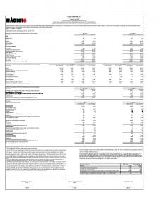
In evaluating the VECM estimated model and taking into consideration that there are four lags in each equation and the difficulty to interpret each coefficient especially because the coefficient signals alternate over time, it is necessary to examine (i) the impulse response function to verify how the dependent variables respond to a shock applied to one or more system equations and/or (ii) the decomposition function of the variance which decomposes the forecasted variance error for each variable in components which may be attributed to each of the endogenous variables. 4.6 IMPULSE RESPONSE FUNCTION The impulse response function permits observing how the model responds over time to shocks applied to the model variables. In this paper, the impulse response function was analyzed over a period of ten years, i.e. forty quarters. Graph 1 shows the time behavior graph of the endogenous variables in response to a shock applied to the Current Assets. It can be seen that in the case of a shock to the CA variable, the FA, LL and even the CA variables tend towards equilibrium more quickly while the NR and CL variables reveal themselves to have a long-term memory. It is interesting to note that the CA, LL and NI variables tend to return to pre-shock levels after oscillations while FA, CL, LL and NR have a change on their levels after the shock.



34


Graphs of the impulse response functions in relation to shocks applied to other accounting variables or to exogenous variables, as well as variance decomposition results are not shown in this paper due to problems of space. 4.7 FORECASTS Based on the estimated VECM model, financial statement forecasts were carried out with the following characteristics: · Ex-post forecasts: 12/31/2002 to 12/31/2006: with the objective of validating the predictive capacity of the model, comparing annual projections with real data (Table 7); · Ex-ante forecasts: 12/31/2007 to 12/31/2010 (Tables 8 and 9). The short-term forecasts demonstrate that the model has a relatively good predictive capacity, being that one of the variables with a larger error prediction was Net Income with a value of 1.37% above what occurred in 2002. For periods of more than one year, the model loses some of its predictive power which is normal, given that other variables that influence the firm’s financial results are not fed into the model. Ex-ante forecasts were done initially considering past observations of endogenous and exogenous variables and also of some assumptions regarding the future performance of exogenous variables carried out by the Central Bank of Brazil through the Focus Report, the Market Report, the market expectations release, including the “Top 5” institutions, Reuters’ data and other considerations of the authors, regarding the future behavior of the variables: the Emerging Market Bond Index plus (Embi+) and the London Interbank Offered Rate - 06 Months, since forecasts from trustworthy publications were not available. The forecasts concerning annual changes of Petrobras accounts were made for the period of 31/12/2007 to 31/12/2010, taking into account a likely scenario involving the exogenous variables. The sample selected for the forecasting refers to the period from 31/03/1990 to 31/12/2006. It was done through a stochastic simulation with 100,000 repetitions in a dynamic solution. The values are in constant currency from December 2006.



35


Response to Nonfactorized One Unit Innovations Response of AC to AC

Response of AP to AC

1.2

0.8

Response of PC to AC

0.2

.5

0.0

.4

-0.2

.3

-0.4

.2

-0.6

.1

0.4

0.0

-0.4

-0.8

.0

-1.0

-.1

-1.2 5

10

15

20

25

30

35

40

-.2 5

Response of ELP to AC

10

15

20

25

30

35

40

5

Response of PL to AC

.4

10

15

20

25

30

35

40

35

40

Response of RLO to AC

0.4

.04

.3

.00 0.0

.2

-.04

.1 -0.4

-.08

.0 -.12

-.1

-0.8 -.16

-.2 -.3

-1.2 5

10

15

20

25

30

35

40

35

40

-.20 5

10

15

20

25

30

35

40

5

10

15

20

25

30

Response of LL to AC

.0

-.1

-.2

5

10

15

20

25

30

Graph 1: Impulse response resulting from a shock in the CA variable. Source: Results of the study. Table 7: Comparison between ex-post forecasts and real data from 31/12/2002 to 31/12/2006 Differences Projections X Real BP 2002 AT -0.01% CA 0.26% RLP -1.25% FA 1.01% PT -0.01% CL -1.21% LL 3.48% EQ -0.58% IS 2002 NR -0.94% CPV + DESP. -1.43% NI 1.37% Source: Results of the study.

2003 1.93% 3.87% -9.05% 8.18% 1.93% -0.92% -16.69% 13.28% 2003 0.22% -2.21% 8.46%


2004 6.46% 16.76% -11.26% 14.07% 6.46% -2.88% -2.08% 16.82% 2004 7.46% 6.48% 11.20%

2005 -5.32% -23.00% 5.25% 0.16% -5.32% -11.60% -10.55% 0.05% 2005 -9.87% -8.02% -16.32%

2006 -1.88% -24.34% 9.41% 5.17% -1.88% 13.65% -3.40% -9.38% 2006 -19.91% -18.92% -23.45%


36


Table 8: Exogenous variable forecasts for 31/12/2007 to 31/12/2010 (nominal values) 31/12/2007 31/12/2008 31/12/2009 31/12/2010 Selic goal defined by Copom 11.50% 10.50% 10.00% 10.00% Exchange rate interest1 R$ 2.15 R$ 2.23 R$ 2.18 R$ 2.22 3.50% 3.50% 3.70% 3.75% Gross Domestic Product2 Wholesale Price Index 4.48% 4.28% 4.25% 4.50% 1 3 Dubai Crude Oil Average Price US$ 62.00 US$ 60.00 US$ 57.00 US$ 53.60 Producer Price Index – PPI2 1.9%3 1.9%3 2.2% 1.9% 4 4 4 208 Bp 192 Bp 177 Bp 163 Bp4 Emerging Market Bond Index Plus - Embi+ London Interbank Offered Rate - 06 Month 5.39%4 5.39%4 5.394 5.39%4 (1) Values for the end of the period; (2) Values during the period of one year; (3) Values forecasted by the authors; (4) Projections by the authors considering a better country risk scenario with 1.00% quarterly from 31/12/2006 and maintaining the Libor at 5.39% annually from 31/12/2006. Source: Focus Report (BCB), projections from 29/12/2006; Reuters forecasts made in April of 2007 and author forecasts. Source: Results of the study. Table 9: Annual account variation forecasts for Petrobras from 31/12/2007 to 31/12/2010 (values in R$ 1.000) BP 2007 2008 2009 2010 AT 11.97% 1.94% 5.93% 5.99% CA -21.00% -22.88% 12.45% 16.04% RLP 32.84% 4.22% 3.64% 1.96% FA 20.05% 10.11% 5.45% 5.32% PT 11.97% 1.94% 5.93% 5.99% CL 25.27% 0.31% 0.54% 2.98% LL -4.71% -3.75% 15.22% 7.26% EQ 10.11% 4.35% 6.74% 7.25% NR -10.57% 0.07% 6.84% 6.87% CPV + DESP. -11.08% 2.53% 1.68% 4.91% NI -8.75% -8.54% 26.99% 13.01% Source: Results of the study.

5. CONCLUSIONS This paper sought to specify and estimate a Vector Auto-Regressive (VAR) model based on the financial statements of a firm, taking into account the influence exogenous economic variables on the chosen firm. In fact, the model developed is a VECM model, given the presence of cointegration among the model’s variables. The firm utilized as the basis for modeling was Petrobras – Petroleo Brasileiro S/A. The model obtained was used to elaborate financial statement forecasts. It was possible to evaluate the relationship among the accounting variables and the impact of economic variables on the economic activity of Petrobras using a correlation matrix of endogenous and exogenous variables and causality analysis by means of a Granger test. Empirically, relevant conclusions were achieved regarding the relationships among the model's variables. A positive and high correlation can be observed between the Current Asset variations and the net operating revenue with the variations of the other accounting variables. BBR, Braz. Bus. Rev. (Engl. ed., Online), Vitória, v. 8, n. 3, Art. 2, p. 20-39, jul. - sep. 2011



37

The empirical correlation observed between the Current Assets and Liabilities corroborates the accounting theory supposition that there should be a congruency between the short-term assets and liabilities. With regard to the Granger causality test, it can be concluded that the variables that precede D(CA) are in order of importance: D(FA); D(CL) and D(EQ). No economic variable revealed itself significant. In relation to the variable D(FA), only exogenous economic variables precede it and are in decreasing order of importance: D(RISK); D(SELIC); D(GDP); and D(EXCHANGE RATE). This means that, investments or disinvestments by a firm are made based on the behavior of these variables. With respect to Liabilities, they would be caused by variations in the Net Operating Revenue and even more significantly, by exchange rate variations. Variables that would have a causal relationship with the variations in the Balance Sheet variables are in order of decreasing importance: D(RISK); D(SELIC); D(EXCHANGE RATE); and D(GDP). With relation to the Net Operating Revenue variations of Petrobras, the only variable that demonstrated having a causal relationship was D(OIL), which makes sense since the price of petroleum is the main component in the firm's income. With respect to Net Profit, two variables revealed themselves to be important in defining future values: D(OIL) and D(NR) which proves empirically that the international oil price and the Net Operating Revenue have influence over Petrobras' profit. The most important conclusion reached empirically by the Granger causality test is that the price of petroleum precedes the Net Operating Revenue and consequently influences the profitability of the firm. In second place, there seems to be empirical evidence that Vector Autoregressive models have a greater forecasting capacity than does multiple equations system models. This fact was described after making the ex-post forecasts for Petrobras' annual accounts for the periods of 31/12/2002 to 31/12/2004 and the consequent comparison with De Medeiros' (2004) study. The ex-post forecasts demonstrate that there is a strong relationship between the variations in the Petrobras accounts with variations in the economic variables. This means that it was possible to verify that since Petrobras is the largest firm in Brazil, its accounts vary much more in accordance with market variations than in accordance with whichever model of management has been adopted.



38


The models’ ex-ante forecasts illustrate a positive trend for Net Income. This conclusion raises considerations about the model's exogenous variables that, in general, predicts a more stable macroeconomic scenario for the country, e.g. a significant increase in the GDP, maintenance of the exchange rate level, stable inflation, diminishing country risk, falling nominal interest rates and a lower international oil price. This means that the variables forecasted carry with them the memory of past turbulence involving exogenous variables and its own endogenous variables. As such, it can be noted that the Net Profit forecasted for 2007 and 2008 has negative growth, despite inverting this tendency from 2010. A fundamentalist analysis of the forecasted accounts reveals relative stability over time. REFERENCES ABRAS, M. A. Finanças Corporativas e Estratégia Empresarial: Turbulência do Ambiente, Alavancagem Financeira e Performance da Firma no Ambiente de Negócios Brasileiros. XXVII EnANPAD – Encontro Anual da ANPAD, Atibaia – SP: Anais…, EnANPAD, setembro, 2003. BROOKS, C. Introductory Econometrics for Finance. Cambridge: Cambridge University Press, 2004. CAMPBELL, J.; SHILLER, R. Cointegration and Tests of Present Value Models, Journal of Political Economy, vol. 95, n. 5, 1987, pp. 1062-1088. DE MEDEIROS, O. R. Modelagem Econométrica das Demonstrações Financeiras. UnB Contábil, vol. 7, n. 1, 2004. DE MEDEIROS, O. R. An Econometric Model of a Firm's Financial Statements. SSRN Working Paper Series, Available at Accessed on March 10, 2005. DICKEY, D.; FULLER, W. A. Distributions of the estimates for autoregressive time series with a unit root. Journal of the American Statistical Association, vol. 74, n. 366, 1979. pp. 427-431. DICKEY, D.; FULLER, W. A. Likelihood Ratio Statistics for Autoregressive Time Series with a Unit Root. Econometrica, vol. 49, n. 4, 1981. pp. 1057-72. ENDERS, W. Applied econometric time series. New York: John Wiley & Sons, Inc., 1995. ENGLE, R.F.; GRANGER, C. W. J. Cointegration and Error-Correction: Representation, Estimation and Testing. Econometrica, vol. 55, n. 2, pp. 251-276, 1987. ENGLE, R.F.; YOO, B.S. Forecasting and Testing in Cointegrated Systems. Journal of Econometrics, vol. 35, n. 1, pp. 143-59, 1987. ERAKER, B. Predicting Asset Returns using Autoregressive Latent Component Models. Available at: Accessed on December 2, 2005.



39


GEROSKI, P. A. The Growth of Firms in Theory and in Practice. London Business School. Available at: Accessed on December 2, 2005. GRANGER, C.W.J. Investigating Causal Relationships by Econometric Models and Crossspectral Methods, Econometrica, vol. 37, n. 3, pp. 424-38, 1969. GUJARATI, D. N. Econometria Básica. São Paulo, Makron Books, 2000. HAMILTON, J. Time Series Analysis. Princeton: Princeton University Press, 1994. HARRIS, R. I. D. Using cointegration analysis in econometric modelling. Hampstead: Prentice Hall, 1995. JOHANSEN, S. Statistical Analysis of Cointegrating Vectors. Journal of Economic Dynamics and Control, vol. 12, n. 2-3,1988. pp. 231-254. JOHANSEN, S.; JUSELIUS, K. Maximum likelihood estimation and inference on cointegration with application to the demand for money. Oxford Bulletin of Economics and Statistics, vol. 52, n. 2, pp.169-209, 1990. LITTERMAN, R. Techniques of Forecasting Using Vector Autoregressions. Federal Reserve Bank of Minneapolis. Working Paper No. 15, 1979. LITTERMAN, R. Forecasting with Bayesian Vector Autoregressions-Five Years of Experience. Journal of Business and Economic Statistics, vol. 4, n. 1, pp. 25-38, 1986. LUTKEPOHL, H. Introduction to multiple time series analysis. Berlin: Springer-Verlag, 2 ed., 1993. MCNEES, S. K. Forecasting Accuracy of Alternatives Techniques: A Comparison of US Macroeconomic Forecasts. Journal of Business and Economic Statistics, vol. 4, n.1, pp. 515, 1986. MUMFORD, K. Strikes and Profits: considering an asymmetric information model. Applied Economics Letters, vol. 3, n. 8, p. 545- 548, 1996. OGAWA, K. Monetary Transmission and Inventory: Evidence from Japanese Balance-Sheet Data by Firm Size. Japanese Economic Review, vol. 53, n. 4, p. 425, 2002. OXELHEIM, L. The Impact of Macroecomonic Variables on Corporate Performance - What Shareholders Ought to Know? SSRN Working Paper Series, Available at SSRN: http://ssrn.com/abstract=1010860, 2002. OXELHEIM, L.; WIHLBORG C. Macroeconomic Uncertainty – International Risks and Opportunities for the Corporation. Chichester: John Wiley, 1987. OXELHEIM, L.; WIHLBORG C. Managing in the Turbulent World Economy – Corporate Performance and Risk Exposure. Chichester: John Wiley, 1997. PEREZ-QUIROS; TIMMERMANN. Firm Size and Cyclical Variations in Stock Returns. Journal of Finance, vol. 55, n. 3, pp. 1229, 2000. SALTZMAN, S. An Econometric Model of a Firm. Review of Economics and Statistics, vol. 49, n. 3, pp. 332-342, 1967. SIMS, C. A. Macroeconomics and Reality, Econometrica, v. 48, n. 1, pp. 1-48, 1980. VERBEEK, M. A Guide to Modern Econometrics. Chischester: John Wiley, 2004.



Modeling and forecasting a firm's financial statements with a VAR

Modeling and forecasting a firm's financial statements with a VAR

Suggest Documents