STRUCTURAL EQUATION MODELING, 7(2), 174–205 Copyright © 2000, Lawrence Erlbaum Associates, Inc.
Modeling Causal Error Structures in Longitudinal Panel Data: A Monte Carlo Study Stephen A. Sivo Center for Assessment and Research Studies James Madison University
Victor L. Willson Department of Educational Psychology Texas A&M University
This research was designed to investigate how much more suitable moving average (MA) and autoregressive-moving average (ARMA) models are for longitudinal panel data in which measurement errors correlate than AR, quasi-simplex, and 1-factor models. The conclusions include (a) when testing for a stochastic process hypothesized to occur in a longitudinal data set, testing for other processes is necessary, because incorrect models often fit other processes well enough to be deceiving; (b) when measurement error correlations are flagged to be relatively high in panel data, the fit and propriety of an MA or ARMA model should be considered and compared to the fit and propriety of other models; (c) when an MA model is fit to AR data, measurement error correlations may nonetheless be deceptively high, though fortunately MA model fit indexes are almost always lower than those for an AR model; and (d) the assumption that longitudinal panel data always contain measurement error correlations is patently false. In summary, whenever evaluating longitudinal panel data, the fit, propriety, and parsimony of all 5 models should be considered jointly and compared before a particular model is endorsed as most suitable.
Although the practice of testing longitudinal panel data for quasi-simplex structures has grown in the social sciences over the last 20 years, alternative models have seldom been considered (Marsh, 1993). In response to the dearth of alternative models examined, Marsh set forth an investigation that offers and tests a competing model: the one-factor model. Indeed, Marsh went beyond simply testing the Requests for reprints should be sent to Stephen A. Sivo, Center for Assessment & Research Studies, James Madison University, Harrisonburg, VA 22807. E-mail:
[email protected]
MODELING CAUSAL ERROR STRUCTURES
175
one-factor model against the traditionally used simplex models. Concerned about potentially serious limitations in both the simplex and one-factor models in single indicator form, Marsh, as we have interpreted his article, compared the relative performance of their multiple indicator counterparts as well. The one-factor and simplex multiple indicator models differed in that each item on a test is modeled explicitly as a manifest variable. For example, a four-item test administered over six occasions would give four indicators per occasion. Both quasi-simplex and one-factor, single-indicator models are used when the focus of the longitudinal research is on the stability of individual differences over time. As such, both models are designed to answer “why the true scores representing the same construct are not perfectly correlated from one occasion to the next” (Marsh, 1993, p. 158). The quasi-simplex model suggests that each occasion has its own true score plus some random measurement error; the one-factor model suggests that each occasion shares the same true score plus some random measurement error (much as the classical true score model posits, Xi = Ti + Ei). Both models are alike in that they assume that measurement errors across occasions are random. When this assumption is false, neither model suffices, and motive to posit other models arises. Indeed, the assumption that measurement errors in longitudinal panel data are random across occasions often enough proves to be false. Several researchers have reported that correlated measurement errors in longitudinal panel data are commonplace (e.g., Jöreskog, 1979, 1981; Jöreskog & Sörbom 1977, 1989; Marsh, 1993; Marsh & Grayson, 1994; Rogosa, 1979). In fact, Marsh (1993) identified substantive measurement error correlations in many of his own data sets as a part of his investigation. Such findings signal the need for alternatives to either the quasi-simplex or the one-factor, single-indicator models. Marsh’s solution, as we understand it, was to specify simplex and one-factor models in their multiple indicator form, allowing measurement errors to correlate. Although potentially useful, other solutions should be entertained as well. It so happens that models specifying correlated errors already exist. Moreover, such models belong to the same family of stochastic models to which the quasi-simplex model belongs. These time series models may prove proper when measurement errors are found to correlate across occasions in longitudinal panel data. If such models are sufficient in representing measurement errors that correlate in a data set, a multiple indicator counterpart would be unnecessary.1
1It should be pointed out that Marsh does not necessarily agree with our approach. Previously, in an article reacting to Marsh and Hau (1996), we recommended the use of time series models for analyzing longitudinal panel data as an alternative to Marsh’s multiple indicator models (see Sivo & Willson, 1998). Marsh and Hau (1998) had an opportunity to rebut our proposed remedy in the same series. For more on this topic, see The Journal of Experimental Education, Volume 66, Issue 3. The series is entitled “The Role of Parsimony in Assessing Model Fit in Structural Equation Modeling.”
176
SIVO AND WILLSON
FITTING TIME SERIES MODELS TO A LONGITUDINAL PANEL DATA Broadly, times series data may often be modeled for two distinct stochastic processes: autoregressive (AR) and moving average (MA; Box & Jenkins, 1976). AR models are constructed to allow the current value of a time series to be expressed as a function of previous values of the same time series: Xt = φ1 Xt – 1 + φ2 Xt – 2 + ... + φp Xt – p + εt where Xt denotes an observed score taken on some occasion (t) deviated from the original level X0 of the series, ε denotes error associated with a given occasion (t), and φ denotes a correlation among temporally ordered scores at some lag (e.g., t – 1 = a lag of 1, t – 2 = a lag of 2). MA models are constructed to allow the current value of a time series to be expressed as a function of autocorrelated errors: Xt = εt – θ1 εt – 1 – θ2 εt – 2 – ... – θq εt – q where Xt denotes an observed score taken on some occasion (t) deviated from the original level X0 of the series, ε denotes error associated with a given occasion (t), and θ denotes a correlation among errors at some lag (e.g., t – 1 = a lag of 1, t – 2 = a lag of 2). MA models suggest that errors correlate across occasions at some lag. For example, a lag 1 MA model would have the error for the first occasion correlate with the second occasion error, and the second occasion error correlate with the third occasion error. However, the first occasion error would not be correlated with the third occasion error. The possibility of both processes being present in the same data lends support for ARMA models: Xt = φ1 Xt – 1 + φ2 Xt – 2 + ... + φp Xt – p – θ1 εt – 1 – θ2 εt – 2 – ... – θq εt – q + εt Hershberger, Corneal, and Molenaar (1994) as well as Hershberger, Molenaar, and Corneal (1996) provide fairly recent examples of situations in which AR, MA, and ARMA models may be fit to time series data using structural equation modeling (SEM). In an article concerning how to use SEM to test time series models against longitudinal panel data, Willson (1995b) noted that the basic AR(1) model is but a restricted form of Marsh’s (1993) simplex model. Willson further indicated that Marsh did not test a model that assumes an MA process, wherein the errors, rather than the scores, propagate, although he suggested that the errors may possess an MA structure if a lag 1 autocorrelation among the errors were to be found. Not only is it plausible to observe whether stochastic MA or ARMA models fit data with
MODELING CAUSAL ERROR STRUCTURES
177
correlated measurement errors, but it is necessary. Not allowing the errors to correlate inflates the association between each manifest variable with its respective latent variable (Marsh, 1993) and greatly inflate Type I error rates for any associated tests (Box & Jenkins, 1976). Given that measurement error correlations are often found in longitudinal panel data, it is surprising that simple MA and ARMA models have not been used as widely as the quasi-simplex model, especially when all three models belong to the same general class of stochastic models. Perhaps the reason time series models specifying correlated errors have not been used is that, [While] econometricians have concentrated on the linear simultaneous equation model, in which there are stochastic disturbances in equations (‘shocks’) but not on measurement errors in variables (‘errors’)[,] … other social scientists—e.g., psychometricians and statistical sociologists—have focused their attention on errors-in-variables models in the form of true score theory and factor analysis. (Geraci, 1977, p. 163)
Presumably, “other social scientists” have not focused much attention on stochastic disturbances. Given the objective of choosing the most parsimonious and theory-driven model, motive for an investigation that demonstrates the applicability of such time series models exists. The intention of this study was to determine whether MA or ARMA models fit two longitudinal data sets previously thought to possess quasi-simplex structures better than the quasi-simplex, one-factor, or AR models. Three facts motivated this investigation: (a) Longitudinal data reportedly evidence measurement error correlations so routinely that assuming such correlations is thought advisable, given the consequences of not doing so (see Jöreskog, 1979, 1981; Jöreskog & Sörbom 1977, 1989; Marsh, 1993; Rogosa, 1979); (b) many previously published longitudinal studies concerning one variable measured over time evaluate only the fit of simplex and quasi-simplex models, although neither model includes the specification of measurement error correlations (Marsh, 1993); and (c) the fit of the quasi-simplex model to such data sets, in each case, was not compared to rival models before their endorsement as being suitable probably because, as Marsh argued, the use of the quasi-simplex model has not been scrutinized sufficiently. Based on the aforementioned arguments, the following research questions are posed: 1. Do the quasi-simplex, one-factor, AR, MA, and ARMA models fit their respective, generated data types as well as or better than any of the other five competing models? 2. Do the MA or ARMA models fit selected longitudinal data sets expected to possess a quasi-simplex structure with correlated measurement errors as well as or better than the quasi-simplex, one-factor, or AR models?
178
SIVO AND WILLSON
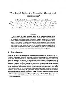
METHOD Data Description Five eight-occasion data sets were artificially generated using the SAS RANNOR function (SAS Institute, 1989) so as to favor the fit of each of the five models under study: the one-factor, quasi-simplex, AR, MA, and ARMA. The RANNOR function generates an observation of a normal random variable possessing a mean of zero and a standard deviation of one. Each data set consisted of 500 cases. Uncorrelated true score or error processes were chosen to serve as a control condition. In generating one-factor data, the goal was to produce observations for eight occasions that possess a common factor (the same true score) plus some degree of error, independent of occasion. The one-factor data sets were generated to have a reliability of .00, .50, .70, or .90 at each occasion. Data possessing a quasi-simplex process was generated to have observations for eight occasions that possess two related factors (true scores, different though related) plus some degree of latent error, in addition to some degree of measurement error (idiosyncratic to occasion). The quasi-simplex data sets were constructed at .00, .33, .67, or .85 lag parameter value. Data possessing an AR(1) process was generated to have observations for eight occasions in which the first observed score was the only exogenous variable, having direct influence on the second observed score. Eight sets of scores were generated so that an observed score was a function of a previous score plus a degree of random error with lag parameter values of .00, .33, .67, or .85. Data possessing an MA(1) process had observations for eight occasions in which lag 1 measurement errors were correlated according to the fixed parameter values .00, .33, .67, or .85. The model implies that errors are correlated at lag 1. To accomplish this, adjacent errors must have a unique relationship that does not exist between other pairs. In other words, for the MA(1) process, only errors belonging to sequentially adjacent occasions are correlated. Thus, a unique error source influences each error at a given occasion, and that error source serves as that which is correlated with the following error (see Figure 1). The one-factor component of the MA data was generated to have a .00, .50, .70, or .90 reliability at each occasion. Finally, the ARMA program was written so that an observed score was a function of a preceding observed score (AR parameter values = .00, .33, .67, and .85) plus a random error component and a correlated error component (MA parameter values = .00, .30, .60, and .80). For heuristic purposes, two data sets were used for this investigation. Both of the data sets were selected from previously published research investigating the quasi-simplex property in longitudinal data: Mukherjee two-hand proficiency six-wave data (N = 152; cited in Bock & Bargmann, 1966), and Humphreys’ eight-wave college academic success matrix (1968). All of the five models were fit to the two real data sets. Results obtained for each data set were interpreted in light of the simulation findings.
MODELING CAUSAL ERROR STRUCTURES
FIGURE 1
179
Five models tested against the longitudinal data sets.
Procedures for the Analysis All five models (i.e., the quasi-simplex, one-factor, AR, MA, and ARMA; see Figure 1) were estimated using the MVS mainframe version of SAS Institute’s (1989) PROC Covariance Analysis of Linear Structural Equations (CALIS) line equations. For each of the 155 research situations, data were generated and the CALIS procedure was invoked within a macro set at 200 replications.
180
SIVO AND WILLSON
To successfully complete the following investigation, all five models (i.e., the quasi-simplex, one-factor, AR, MA, and ARMA) were assessed for adequate fit, propriety, and parsimony. To determine whether a given model sufficiently fit a data set, the values of three fit indexes were examined (the CFI, TLI, and NFI). By convention, a fit index is considered sufficiently high when its value equals or exceeds .90. Next, the propriety of a solution generated for a model was evaluated according to several criteria, including the behavior of the parameter estimates and associated standard errors, model identification, and the iterative estimation procedure’s attainment of successful convergence. Finally, when two or more models both fit well and attained proper solutions, the models were evaluated on the basis of parsimony. It should be noted that equality constraints for the models were placed on the errors when testing the fit of the quasi-simplex models to the single indicator data so as to eliminate indeterminacies (see Jöreskog, & Sörbom, 1989). The first and the last two errors across time were constrained to be equal. The line equations option in the CALIS procedure was used to analyze the data in our investigation. The one-factor program was written so that the same true score for each observation was present in the eight manifest variables (without constraints imposed) plus an independent error (Appendix A). The quasi-simplex program was written so that each of the eight manifest variables equaled a true score plus an independent measurement error (e.g., A = T + E1, B = T + E2 …). Following these eight equations, more equations were written so that the last seven true scores, in order of occasion, equaled the previous true score plus some latent error (see Appendix B). The AR program, on the other hand, was written so that the first observed score was the only exogenous variable, having direct influence on the second observed score plus some degree of error (see Appendix C). The beta coefficients for all eight occasions were constrained to equal the first beta coefficient in the model. The MA program was written so that each of the eight manifest variables equaled the true score estimated for the first manifest variable (i.e., they were constrained) plus some measurement error. Afterward, the errors were correlated for the first lag (see Appendix D), and all measurement error correlations were constrained as equal to the correlation between the first and second errors in the series. The ARMA program was written in the same manner as the AR program, except the measurement errors were allowed to correlated at the first lag, with all error correlations constrained to equal the first error correlation in the series. RESULTS Fitting the Five Models to the Simulated Data In most cases, the models matching the generated data types fit better than any of the four remaining models; however, often the competing models fit nearly as well (see Table 1). Supplementary information generated for the analysis had to be con-
181
Factor(.90) Factor(.90) Factor(.90) Factor(.90) Factor(.90) Factor(.70) Factor(.70) Factor(.70) Factor(.70) Factor(.70) Factor(.50) Factor(.50) Factor(.50) Factor(.50) Factor(.50) Qsimplex Qsimplex Qsimplex Qsimplex Qsimplex AR AR AR AR AR MA(.90) MA(.90)
Pseudo Data
no lag no lag no lag no lag no lag no lag no lag no lag no lag no lag no lag no lag no lag no lag no lag .85 .85 .85 .85 .85 .85 .85 .85 .85 .85 .85 .85
Lag 1 Parameter Factor Qsimplex AR MA ARMA Factor Qsimplex AR MA ARMA Factor Qsimplex AR MA ARMA Factor Qsimplex AR MA ARMA Factor Qsimplex AR MA ARMA Factor Qsimplex
Model 1.000 (0.997, 1.000) 1.000 (0.997, 1.000) 0.823 (0.802, 0.847) 1.000 (0.996, 1.000) 0.996 (0.990, 1.000) 0.999 (0.994, 1.000) 0.999 (0.993, 1.000) 0.708 (0.668, 0.741) 0.999 (0.992, 1.000) 0.972 (0.954, 0.985) 0.998 (0.988, 1.000) 0.999 (0.989, 1.000) 0.597 (0.514, 0.653) 0.998 (0.987, 1.000) 0.907 (0.859, 0.938) 0.839 (0.788, 0.869) 0.999 (0.996, 1.000) 0.953 (0.936, 0.971) 0.934 (0.898, 0.956) 0.997 (0.989, 1.000) 0.724 (0.621, 0.809) 0.998 (0.990, 1.000) 1.000 (0.992, 1.000) 0.893 (0.840, 0.945) 1.000 (0.995, 1.000) 0.860 (0.781, 0.932) 0.931 (0.884, 0.972)
CFI 1.000 (0.996, 1.002) 1.000 (0.994, 1.003) 0.817 (0.794, 0.841) 1.000 (0.996, 1.002) 0.995 (0.990, 1.000) 1.000 (0.992, 1.006) 1.000 (0.988, 1.006) 0.697 (0.656, 0.731) 1.000 (0.991, 1.006) 0.970 (0.950, 0.984) 1.000 (0.983, 1.011) 1.000 (0.980, 1.012) 0.582 (0.496, 0.641) 1.000 (0.986, 1.011) 0.900 (0.848, 0.934) 0.775 (0.703, 0.817) 1.000 (0.993 ,1.006) 0.951 (0.933, 0.970) 0.929 (0.891, 0.953) 0.997 (0.988, 1.002) 0.614 (0.470, 0.732) 0.998 (0.981, 1.013) 1.001 (0.992, 1.004) 0.884 (0.828, 0.941) 1.002 (0.995, 1.006) 0.803 (0.694, 0.904) 0.872 (0.783, 0.949)
TLI
TABLE 1 The Fit of Each Model to Each Simulated Data Set: 200 Replications
0.997 (0.995, 0.999) 0.998 (0.994, 0.999) 0.820 (0.798, 0.844) 0.996 (0.992, 0.998) 0.992 (0.987, 0.997) 0.994 (0.988, 0.998) 0.995 (0.989, 0.999) 0.702 (0.662, 0.735) 0.992 (0.983, 0.998) 0.964 (0.946, 0.979) 0.988 (0.976, 0.996) 0.992 (0.981, 0.998) 0.588 (0.505, 0.644) 0.984 (0.970, 0.995) 0.893 (0.844, 0.927) 0.836 (0.785, 0.865) 0.996 (0.993, 0.999) 0.947 (0.930, 0.965) 0.928 (0.893, 0.950) 0.991 (0.982, 0.996) 0.722 (0.619, 0.807) 0.991 (0.982, 0.999) 0.997 (0.988, 1.000) 0.889 (0.836, 0.942) 0.998 (0.991, 1.000) 0.851 (0.775, 0.923) 0.925 (0.879, 0.966) (continued)
NFI
182
Lag 1 Parameter
.85 .85 .85 .85 .85 .85 .85 .85 .85 .85 .85 .85 .85 .85 .85 .85 .85 .85 .85/.80 .85/.80 .85/.80 .85/.80 .85/.80 .67 .67 .67 .67 .67
Pseudo Data
MA(.90) MA(.90) MA(.90) MA(.70) MA(.70) MA(.70) MA(.70) MA(.70) MA(.50) MA(.50) MA(.50) MA(.50) MA(.50) MA(.00) MA(.00) MA(.00) MA(.00) MA(.00) ARMA ARMA ARMA ARMA ARMA Qsimplex Qsimplex Qsimplex Qsimplex Qsimplex
AR MA ARMA Factor Qsimplex AR MA ARMA Factor Qsimplex AR MA ARMA Factor Qsimplex AR MA ARMA Factor Qsimplex AR MA ARMA Factor Qsimplex AR MA ARMA
Model 0.868 (0.793, 0.920) 0.998 (0.978, 1.000) 0.913 (0.863, 0.956) 0.613 (0.476, 0.740) 0.892 (0.826, 0.939) 0.870 (0.820, 0.917) 0.999 (0.979, 1.000) 0.889 (0.833, 0.936) 0.427 (0.321, 0.546) 0.933 (0.880, 0.970) 0.788 (0.708, 0.873) 0.999 (0.978, 1.000) 0.897 (0.847, 0.931) 0.337 (0.278, 0.455) 0.995 (0.957, 1.000) 0.606 (0.481, 0.685) 0.997 (0.966, 1.000) 0.874 (0.818, 0.934) 0.613 (0.546, 0.691) 1.000 (0.996, 1.000) 0.945 (0.922, 0.963) 0.863 (0.805, 0.904) 1.000 (0.995, 1.000) 0.707 (0.642, 0.762) 1.000 (0.995, 1.000) 0.981 (0.963, 0.993) 0.896 (0.857, 0.926) 0.998 (0.990, 1.000)
CFI
TABLE 1 (Continued)
0.863 (0.785, 0.917) 1.001 (0.976, 1.012) 0.907 (0.852, 0.953) 0.459 (0.266, 0.636) 0.799 (0.675, 0.885) 0.865 (0.814, 0.914) 1.003 (0.978, 1.011) 0.881 (0.820, 0.931) 0.197 (0.049, 0.365) 0.875 (0.776, 0.944) 0.780 (0.697, 0.869) 1.003 (0.976, 1.012) 0.889 (0.836, 0.926) 0.072 (–0.010, 0.237) 0.996 (0.920, 1.015) 0.591 (0.462, 0.673) 1.001 (0.963, 1.016) 0.864 (0.804, 0.929) 0.458 (0.365, 0.568) 1.000 (0.993, 1.003) 0.942 (0.919, 0.962) 0.852 (0.790, 0.896) 1.000 (0.994, 1.003) 0.589 (0.499, 0.666) 1.000 (0.990, 1.008) 0.981 (0.962, 0.993) 0.888 (0.846, 0.921) 0.998 (0.990, 1.005)
TLI
0.857 (0.782, 0.909) 0.989 (0.967, 0.998) 0.902 (0.851, 0.945) 0.610 (0.474, 0.734) 0.887 (0.821, 0.933) 0.859 (0.810, 0.905) 0.990 (0.968, 0.999) 0.879 (0.824, 0.925) 0.425 (0.321, 0.543) 0.927 (0.875, 0.963) 0.778 (0.699, 0.863) 0.990 (0.968, 0.999) 0.886 (0.837, 0.920) 0.336 (0.278, 0.451) 0.989 (0.947, 0.998) 0.596 (0.472, 0.675) 0.983 (0.949, 0.999) 0.860 (0.805, 0.921) 0.612 (0.545, 0.690) 0.998 (0.994, 1.000) 0.942 (0.919, 0.960) 0.860 (0.803, 0.901) 0.997 (0.992, 0.999) 0.703 (0.638, 0.757) 0.995 (0.989, 0.999) 0.972 (0.954, 0.984) 0.888 (0.850, 0.918) 0.989 (0.980, 0.995)
NFI
183
AR AR AR AR AR MA(.90) MA(.90) MA(.90) MA(.90) MA(.90) MA(.70) MA(.70) MA(.70) MA(.70) MA(.70) MA(.50) MA(.50) MA(.50) MA(.50) MA(.50) MA(.00) MA(.00) MA(.00) MA(.00) MA(.00) ARMA ARMA ARMA ARMA ARMA Qsimplex
.67 .67 .67 .67 .67 .67 .67 .67 .67 .67 .67 .67 .67 .67 .67 .67 .67 .67 .67 .67 .67 .67 .67 .67 .67 .67/.60 .67/.60 .67/.60 .67/.60 .67/.60 .33
Factor Qsimplex AR MA ARMA Factor Qsimplex AR MA ARMA Factor Qsimplex AR MA ARMA Factor Qsimplex AR MA ARMA Factor Qsimplex AR MA ARMA Factor Qsimplex AR MA ARMA Factor
0.631 (0.516, 0.734) 0.999 (0.995, 1.000) 1.000 (0.995, 1.000) 0.879 (0.806, 0.951) 0.999 (0.985, 1.000) 0.849 (0.769, 0.913) 0.929 (0.878, 0.967) 0.884 (0.841, 0.932) 0.999 (0.981, 1.000) 0.921 (0.864, 0.965) 0.610 (0.534, 0.691) 0.897 (0.840, 0.946) 0.854 (0.779, 0.923) 0.998 (0.984, 1.000) 0.886 (0.825, 0.946) 0.424 (0.330, 0.540) 0.931 (0.854, 0.967) 0.769 (0.713, 0.842) 0.999 (0.990, 1.000) 0.885 (0.838, 0.936) 0.326 (0.145, 0.438) 0.992 (0.948, 1.000) 0.634 (0.541, 0.737) 0.998 (0.959, 1.000) 0.891 (0.836, 0.943) 0.458 (0.368, 0.530) 0.999 (0.992, 1.000) 0.854 (0.808, 0.896) 0.839 (0.801, 0.885) 0.997 (0.982, 1.000) 0.530 (0.414, 0.638)
0.483 (0.323, 0.627) 1.007 (0.990, 1.015) 1.002 (0.989, 1.007) 0.870 (0.791, 0.947) 1.003 (0.984, 1.008) 0.789 (0.677, 0.879) 0.868 (0.773, 0.938) 0.880 (0.835, 0.929) 1.002 (0.979, 1.010) 0.915 (0.854, 0.963) 0.454 (0.347, 0.567) 0.808 (0.702, 0.898) 0.849 (0.771, 0.921) 1.001 (0.982, 1.009) 0.877 (0.812, 0.942) 0.194 (0.061, 0.356) 0.870 (0.728, 0.938) 0.760 (0.702, 0.836) 1.002 (0.989, 1.010) 0.877 (0.826, 0.931) 0.056 (–0.197, 0.214) 0.987 (0.902, 1.012) 0.620 (0.524, 0.727) 1.004 (0.956, 1.020) 0.882 (0.824, 0.938) 0.241 (0.116, 0.343) 0.999 (0.986, 1.003) 0.849 (0.800, 0.892) 0.827 (0.785, 0.876) 0.996 (0.980, 1.000) 0.341 (0.180, 0.493)
0.628 (0.514, 0.731) 0.995 (0.980, 0.999) 0.994 (0.980, 0.999) 0.873 (0.800, 0.944) 0.996 (0.976, 1.000) 0.843 (0.764, 0.907) 0.924 (0.874, 0.961) 0.875 (0.832, 0.922) 0.992 (0.971, 0.999) 0.912 (0.855, 0.956) 0.606 (0.531, 0.686) 0.894 (0.836, 0.940) 0.845 (0.771, 0.914) 0.991 (0.974, 0.999) 0.877 (0.817, 0.937) 0.422 (0.329, 0.537) 0.925 (0.849, 0.961) 0.761 (0.705, 0.833) 0.991 (0.977, 0.997) 0.876 (0.828, 0.926) 0.325 (0.148, 0.435) 0.983 (0.936, 0.996) 0.622 (0.532, 0.724) 0.986 (0.944, 0.999) 0.876 (0.821, 0.927) 0.457 (0.368, 0.529) 0.997 (0.990, 1.000) 0.851 (0.804, 0.893) 0.836 (0.798, 0.882) 0.993 (0.978, 0.996) 0.523 (0.411, 0.630) (continued)
184
Lag 1 Parameter
.33 .33 .33 .33 .33 .33 .33 .33 .33 .33 .33 .33 .33 .33 .33 .33 .33 .33 .33 .33 .33 .33 .33 .33 .33 .33 .33
Pseudo Data
Qsimplex Qsimplex Qsimplex Qsimplex AR AR AR AR AR MA(.90) MA(.90) MA(.90) MA(.90) MA(.90) MA(.70) MA(.70) MA(.70) MA(.70) MA(.70) MA(.50) MA(.50) MA(.50) MA(.50) MA(.50) MA(.00) MA(.00) MA(.00)
Qsimplex AR MA ARMA Factor Qsimplex AR MA ARMA Factor Qsimplex AR MA ARMA Factor Qsimplex AR MA ARMA Factor Qsimplex AR MA ARMA Factor Qsimplex AR
Model 0.998 (0.981, 1.000) 0.995 (0.973, 1.000) 0.898 (0.845, 0.944) 0.996 (0.972, 1.000) 0.491 (0.349, 0.665) 1.000 (1.000, 1.000) 0.998 (0.967, 1.000) 0.900 (0.774, 0.993) 0.999 (0.971, 1.000) 0.827 (0.761, 0.899) 0.911 (0.871, 0.947) 0.904 (0.861, 0.949) 0.999 (0.993, 1.000) 0.908 (0.873, 0.947) 0.612 (0.503, 0.708) 0.889 (0.833, 0.923) 0.808 (0.729, 0.882) 0.999 (0.992, 1.000) 0.861 (0.815, 0.915) 0.514 (0.379, 0.627) 0.909 (0.833, 0.949) 0.798 (0.709, 0.856) 0.999 (0.983, 1.000) 0.876 (0.782, 0.922) 0.306 (0.192, 0.388) 0.997 (0.978, 1.000) 0.761 (0.540, 0.924)
CFI
TABLE 1 (Continued)
1.000 (0.965, 1.020) 0.997 (0.972, 1.013) 0.890 (0.833, 0.940) 0.998 (0.970, 1.014) 0.287 (0.089, 0.531) 1.011 (1.001, 1.017) 1.005 (0.966, 1.023) 0.892 (0.757, 0.992) 1.008 (0.969, 1.023) 0.758 (0.665, 0.859) 0.835 (0.759, 0.901) 0.900 (0.856, 0.948) 1.001 (0.992, 1.006) 0.900 (0.864, 0.943) 0.457 (0.304, 0.591) 0.792 (0.688, 0.856) 0.800 (0.719, 0.878) 1.001 (0.991, 1.006) 0.850 (0.801, 0.909) 0.319 (0.131, 0.478) 0.830 (0.688, 0.905) 0.791 (0.699, 0.851) 1.002 (0.982, 1.009) 0.866 (0.766, 0.915) 0.028 (–0.131, 0.143) 1.003 (0.959, 1.027) 0.753 (0.523, 0.922)
TLI
0.987 (0.967, 0.996) 0.973 (0.946, 0.989) 0.877 (0.825, 0.921) 0.975 (0.950, 0.987) 0.487 (0.348, 0.658) 0.996 (0.991, 0.999) 0.985 (0.947, 0.998) 0.883 (0.760, 0.974) 0.988 (0.949, 0.999) 0.823 (0.758, 0.895) 0.908 (0.868, 0.944) 0.898 (0.856, 0.944) 0.995 (0.987, 0.999) 0.902 (0.867, 0.942) 0.610 (0.501, 0.705) 0.885 (0.830, 0.919) 0.802 (0.723, 0.877) 0.994 (0.984, 0.999) 0.854 (0.810, 0.909) 0.512 (0.378, 0.624) 0.904 (0.829, 0.944) 0.790 (0.703, 0.848) 0.992 (0.973, 0.998) 0.867 (0.775, 0.913) 0.305 (0.195, 0.384) 0.985 (0.960, 0.998) 0.739 (0.524, 0.898)
NFI
185
MA(.00) MA(.00) ARMA ARMA ARMA ARMA ARMA Qsimplex Qsimplex Qsimplex Qsimplex Qsimplex AR AR AR AR AR MA(.90) MA(.90) MA(.90) MA(.90) MA(.90) MA(.70) MA(.70) MA(.70) MA(.70) MA(.70) MA(.50) MA(.50) MA(.50) MA(.50)
.33 .33 .33/.30 .33/.30 .33/.30 .33/.30 .33/.30 .00 .00 .00 .00 .00 .00 .00 .00 .00 .00 .00 .00 .00 .00 .00 .00 .00 .00 .00 .00 .00 .00 .00 .00
MA ARMA Factor Qsimplex AR MA ARMA Factor Qsimplex AR MA ARMA Factor Qsimplex AR MA ARMA Factor Qsimplex AR MA ARMA Factor Qsimplex AR MA ARMA Factor Qsimplex AR MA
0.996 (0.932, 1.000) 0.902 (0.769, 0.953) 0.312 (0.240, 0.447) 0.999 (0.991, 1.000) 0.816 (0.751, 0.891) 0.877 (0.831, 0.948) 0.986 (0.968, 0.996) 0.886 (–0.270, 1.000) 0.096 (–0.591, 1.000) –0.296(–21.87, 1.000) –0.441(–17.23, 1.000) –0.424(–38.69, 1.000) 0.346 (–22.17, 1.000) 1.000 (1.000, 1.000) 0.441 (–21.87, 45.02) 0.508 (–0.832, 1.000) 0.290 (–15.70, 1.000) 0.999 (0.994, 1.000) 0.999 (0.996, 1.000) 0.825 (0.795, 0.858) 1.000 (0.994, 1.000) 0.996 (0.993, 0.999) 0.998 (0.984, 1.000) 0.999 (0.995, 1.000) 0.710 (0.620, 0.779) 0.999 (0.987, 1.000) 0.972 (0.957, 0.981) 0.997 (0.972, 1.000) 0.994 (0.977, 1.000) 0.603 (0.486, 0.697) 0.999 (0.980, 1.000)
1.007 (0.927, 1.031) 0.895 (0.752, 0.950) 0.036 (–0.063, 0.226) 1.000 (0.983, 1.006) 0.809 (0.741, 0.887) 0.868 (0.818, 0.944) 0.985 (0.965, 0.996) –7.623(–1249.14, 95.24) 0.332(–9.483, 6.550) 0.210(–22.71, 67.15) 0.059(18.63, 19.051) –0.209 (–41.75, .3.96) 0.492 (–31.4, 45.75) 1.017 (1.006, 1.020) 0.226 (0.000, 0.958) –0.025 (–27.42, 51.04) 0.094 (–38.31, 32.39) 1.000 (0.992, 1.003) 1.000 (0.992, 1.004) 0.818 (0.787, 0.853) 1.001 (0.993, 1.003) 0.996 (0.993, 0.999) 0.999 (0.978, 1.007) 1.001 (0.991, 1.007) 0.700 (0.606, 0.771) 1.002 (0.986, 1.008) 0.970 (0.953, 0.980) 0.999 (0.961, 1.016) 0.992 (0.958, 1.017) 0.588 (0.467, 0.686) 1.004 (0.978, 1.015)
0.978 (0.908, 0.998) 0.876 (0.746, 0.930) 0.311 (0.241, 0.446) 0.996 (0.987, 0.999) 0.810 (0.745, 0.885) 0.871 (0.826, 0.941) 0.979 (0.961, 0.990) 0.459 (0.211, 0.667) 0.438 (0.113, 0.750) 0.032 (5.962, 0.258) 0.057 (3.361, 0.420) 0.067 (0.000, 0.383) 0.395 (0.157, 0.860) 0.998 (0.993, 1.000) 0.007 (0.144, 0.112) 0.288 (–38.31, 32.39) 0.230 (0.000, 0.906) 0.997 (0.991, 1.000) 0.998 (0.994, 1.000) 0.822 (0.792, 0.855) 0.997 (0.990, 0.999) 0.992 (0.867, 0.942) 0.993 (0.979, 0.999) 0.996 (0.991, 0.999) 0.704 (0.614, 0.773) 0.994 (0.979, 0.999) 0.964 (0.948, 0.974) 0.987 (0.961, 0.998) 0.987 (0.971, 0.999) 0.593 (0.477, 0.686) 0.988 (0.964, 0.997) (continued)
186
.00 .00 .00 .00 .00 .00 .00/.00 .00/.00 .00/.00 .00/.00 .00/.00
MA(.50) MA(.00) MA(.00) MA(.00) MA(.00) MA(.00) ARMA ARMA ARMA ARMA ARMA
ARMA Factor Qsimplex AR MA ARMA Factor Qsimplex AR MA ARMA
Model 0.907 (0.880, 0.948) 0.482 (–0.214, 1.000) 0.272 (–1.381, 1.000) 0.709 (0.166, 1.000) 0.127 (–7.083, 1.000) 0.335 (–1.284, 1.000) 0.737 (0.304, 1.000) –1.781 (–4.713, 1.000) 0.298 (–0.243, 1.000) –0.314 (–0.086, 1.000) –0.449 (–0.653,1.000)
CFI 0.900 (0.871, 0.944) 0.090 (–0.854, 1.586) 0.390 (–3.445, 5.262) –5.021 (–105.0, 9.003) –0.304 (–7.704, 3.995) –0.069 (–2.546, 2.455) 0.484 (–2.095, 4.792) –1.636 (–9.663, 4.824) –0.106 (–1.074, 1.132) –3.087 (–43.63, 1.390) 0.265 (–9.552, 16.90)
TLI
0.893 (0.867, 0.934) 0.394 (0.218, 0.611) 0.448 (0.000, 0.811) 0.219 (0.002, 0.574) 0.280 (0.001, 0.887) 0.212 (0.002, 0.751) 0.443 (0.291, 0.709) 0.267 (0.004, 0.663) 0.176 (0.009, 0.540) 0.282 (0.006, 0.786) 0.233 (0.001, 0.744)
NFI
Note. Reliabilities for the Factor and MA data are in parentheses. CFI = comparative fit index; TLI(NNFI) = Tucker–Lewis index; NFI = normed fit index. The lag values of .00, .33, .67, and .85 were chosen for the generation of the quasi-simplex, autoregressive, and moving average processes. Average index values are followed by the minimum and maximum values obtained for the 200 replications for each situation.
Lag 1 Parameter
Pseudo Data
TABLE 1 (Continued)
MODELING CAUSAL ERROR STRUCTURES
187
TABLE 2 Research Question 1: Summary of Model Fit to Generated Data
Simulated Data Process
Reliability
Lag 1 Parameter Value
One factor One factor One factor Quasi-simplex AR MA MA MA MA ARMA Quasi-simplex AR MA MA MA MA ARMA Quasi-simplex AR MA MA MA MA ARMA Quasi-simplex AR
.90 .70 .50 * * .90 .70 .50 .00 * * * .90 .70 .50 .00 * * * .90 .70 .50 .00 * * *
No Lag No Lag No Lag .85 .85 .85 .85 .85 .85 .85/.80 .67 .67 .67 .67 .67 .67 .67/.60 .33 .33 .33 .33 .33 .33 .33/.30 .00 .00
MA MA MA MA ARMA
.90 .70 .50 .00 *
.00 .00 .00 .00 .00/.00
Models Favored by the Results One-factor model One-factor model One-factor model Quasi-simplex model AR model MA model MA model MA model MA model ARMA model Quasi-simplex model AR model MA model MA model MA model MA model ARMA model AR model AR model MA model MA model MA model MA model ARMA model No models fit well Quasi-simplex (improperly) One-factor model One-factor model One-factor model No models fit well No models fit well
Note. Favored models fulfilled three criteria better than all contending models: fit, propriety, and parsimony. This table is structured after Table 1. AR = autoregressive; MA = moving average; ARMA = autoregressive moving average.
sulted before a decision could be made regarding the distinctions between the models. Examination of whether the estimator converged to a proper solution was necessary, as well as determining whether parameter estimates were large enough to justify their inclusion in the model. For example, the fit indexes for all models but the AR were uniformly high when tested against the one-factor data set, regardless
188
SIVO AND WILLSON
of manifest variable reliability. However, closer inspection revealed that the maximum likelihood estimator did not converge to a proper solution for the quasi-simplex model, as evidenced by two to four negative eigenvalues. At any reliability, all 200 trials with new random data sets gave the same results, though the number of negative eigenvalues varied slightly. In each case, the maximum likelihood estimator was not able to properly estimate as many parameters, as negative eigenvalues values were estimated for the latent errors (and not the measurement errors). The standardized solutions omitted one latent variable’s error for each negative eigenvalue calculated. The omission of a latent variable’s error, in turn, left the associated beta pathway with an inflated value. Unlike the result for the quasi-simplex model, the maximum likelihood estimator did converge to a proper solution for the MA and ARMA models. In fact, the MA and ARMA models fit the one-factor data fairly well, both attaining indexes ranging from .970 to 1.011 and .844 to 1.000, respectively. Nonetheless, on reviewing other information, both models could be ruled out. For instance, when comparing the MA model results with the one-factor model results, inspection of the parameter estimates for the correlated errors is important. Review of the correlations, regardless of the reliability that the process was generated to have, reveals that the lag 1 relationship among the measurement errors in MA model is not justifiable (e.g., when reliability = .50; see Table 3). Removing the correlations between the adjacent measurement errors would reduce the model to a constrained one-factor model (all lambdas set as equal to the first in the series). In such a situation, testing the one-factor model (unconstrained) would be a legitimate next step to determine which model fits the data set best. Another clue that the MA model is being fit to one-factor data and not MA data is found when the fit of the one-factor model to MA data is examined. Although the MA model fit the one-factor data well, the one-factor model almost never fit the MA data well (see Table 1). The only exception was when the manifest variables for the MA data possessed a reliability of .90; nevertheless, the LM modifiTABLE 3 Simulated One-Factor Data (Reliability = .50): An MA(1) Model Result Relationship ε2 and ε1 ε3 and ε2 ε4 and ε3 ε5 and ε4 ε6 and ε5 ε7 and ε6 ε8 and ε7 Note.
Lag One Correlation
t value
.0118 .0119 .0122 .0122 .0131 .0129 .0124
0.619 0.619 0.619 0.619 0.619 0.619 0.619
ε = measurement error. MA = moving average.
MODELING CAUSAL ERROR STRUCTURES
189
cation indexes still suggested freeing the lag 1 paths, and the fit indexes are much lower than the fit indexes the MA model received. Partial evidence intimating that an MA process is not in a given data set, despite its high fit indexes, is provided when the one-factor model fits an unknown data set well at all. Likewise, if the MA model sufficiently fits an unknown data set well and the one-factor model did not fit the data set well, one may confidently assert that the data is not one-factor data. Clearly, the indexes for the ARMA model were often nearly as high as the indexes produced for the one-factor model, and the measurement errors correlations were remarkably high, but negative (e.g., –.49). Because all of the measurement error correlations were negative, evidence for an ARMA process may be held suspect, given that all of the covariances in the generated matrix were positive in value. Furthermore, when the reliability of the manifest variables was either .50 or .70, the variances of the endogenous variables descend dramatically and uniformly in value over time (e.g., from .47 to .07 when reliability = .50). This pattern in the variances of the endogenous variables is unlike the patterns found in the variances estimated for the ARMA model when fit to ARMA data. When the ARMA model was fit to ARMA data, regardless of the lagged relationships present in both processes, the variances of the endogenous variables were roughly the same across occasions, although the size of the variances depended on the size of the lagged relationships. More evidence that the ARMA model is being fit to one-factor data and not ARMA data is found when the fit of the one-factor model to ARMA data is noted (see Table 1). As with the fit of the one-factor model to the MA data, the one-factor model fit the ARMA data exceptionally poorly regardless of the lagged true score and measurement error relationships (at .33, .67, or .85). Based on the results, when a one-factor model nearly fits perfectly a given data set (index > .99), the ARMA model is expected to fit reasonably well (index > .90), although the data set is devoid of an ARMA process. Discriminating how well the five models fit the simulated quasi-simplex data sets (lag 1 parameter values: .00, .33, .67, and .85) was achieved in the same manner (see Table 2). As would be expected, the quasi-simplex model fit the generated quasi-simplex data well irrespective of lag value (barring the .00 lag 1 parameter, indicating no process whatsoever). Nonetheless, the quasi-simplex model would not properly fit the .33 parameter quasi-simplex data for 138 of the 200 replications, as evidenced by the resultant negative eigenvalues. The CALIS routine indicated that the central parameter matrix (Phi) had two eigenvalues, both associated with the estimation of the measurement errors. When the one-factor model was fit to the quasi-simplex data set, regardless of the first-order lagged relationships of the true scores, the fit indexes were always low enough to rule it out as one-factor data. Although performing better than the one-factor model, the MA model nearly always fit the quasi-simplex data poorly, regardless of the lag coefficient. The estimated correlations between the
190
SIVO AND WILLSON
adjacent measurement errors were even suitably high, typically in the .30s. In fact, the only clear yet effective way to discern the quasi-simplex data from MA data was to examine how the MA and quasi-simplex models behaved when fit to MA data. Regardless of the lagged relationship between occasions in the MA data or the reliability of the scores generated for each occasion, the MA model received fit indexes at .99 or higher—much higher than the indexes obtained for the MA model fit to the quasi-simplex data. More telling was the fact that the quasi-simplex model, when fit to this same MA data set, received negative eigenvalues associated with the measurement error variances, received inappropriately high beta coefficients, or did both. In fact, regardless of how high or low the lag in the measurement errors, the quasi-simplex model often received many negative eigenvalues, indicating improper solutions. In other words, the quasi-simplex model could not be fit to any true MA data set without receiving an improper solution. When the fit indexes for the AR and ARMA models were studied, the values were large enough to suggest a reasonably good fit to the quasi-simplex data (> .90). Moreover, in both cases the maximum likelihood estimator converged to a proper solution within an appropriate number of iterations. This was not too surprising given that both models, like the quasi-simplex model, postulate that true scores are different though related. In part, the quasi-simplex data-generation procedure favored both the AR and ARMA models, because the quasi-simplex data was generated so that all adjacent pairs of true scores were correlated to the same degree. Although the ARMA model fit the quasi-simplex data well, irrespective of the data’s generated lag, the correlations among the measurement errors estimated for the model were fairly small and negative. Indeed, the estimated correlations for the .85 quasi-simplex data were the highest, averaging around –.28 (see Table 4). This information could suggest that the MA component of the ARMA process was modest. However, the impropriety of an ARMA model fit to a matrix of solely positive correlations is evident when all measurement error correlations estimated for the MA component are negative. TABLE 4 Simulated Quasi-Simplex Data With a .85 Lag: An Example of the ARMA Model Fit Relationship ε2 and ε1 ε3 and ε2 ε4 and ε3 ε5 and ε4 ε6 and ε5 ε7 and ε6 Note.
Lag One Correlation
t value
–.158 –.165 –.165 –.152 –.163 –.167
–7.350 –7.350 –7.350 –7.350 –7.350 –7.350
ε = measurement error. ARMA = autoregressive moving average.
MODELING CAUSAL ERROR STRUCTURES
191
To further rule out that the data has an ARMA or AR process, observation of how the quasi-simplex model fits ARMA or AR data is necessary. When the quasi-simplex model was fit to the ARMA data, irrespective of the lag size for the MA and AR processes, none of the solutions was proper, and one negative eigenvalue for each estimated measurement error was received. This result implies that when both an ARMA and quasi-simplex model fit an unknown data set well, the possibility that the data possesses an ARMA process is suspect. When the quasi-simplex model was fit to the generated AR data, irrespective of the AR lag size, the solutions were improper, the estimated measurement errors received small t values, or both of these occurred. When the quasi-simplex model was fit to the AR data generated with .33, .67, or .85 lag 1 parameter values, the t values for all of the measurement errors were lower than .90. Such small t values flag the measurement errors for removal. This result is not surprising given that the AR model may be thought of as a conservative simplex model. Reviewing the fit of the five models to the simulated AR data sets (lag 1 parameter values: .00, .33, .67, and .85) revealed that the one-factor model never received a fit index above .809, and, as previously discussed, the quasi-simplex model fit well, though either improperly or with measurement errors so small that the t values recommend their omission. The MA model on average received fit indexes less than .90, when the AR data possessed a lag 1 parameter value of .67 or.85. When fit to AR(1) data with a .33 lag, the MA model did receive indexes as high as .99, although the average value was less than .90 and could turn up as low as .774. To eliminate the possibility that an MA process exists in a data set, the fit of the AR model to MA data must be considered. Regardless of the lag present in the MA data set, the AR model usually fit the MA data set too poorly to suggest the presence of an AR process (especially when compared to the fit of the MA model). The AR model’s fit to the MA(1) data with a .33 lag value approached .95 when the reliability of the generated data was .90. So, if both an MA and AR model fit an unknown data set very well (>.97), more than likely, the data set does not have an MA process. This is important to consider given that the measurement error correlations estimated for the MA model fit to the AR data were fairly high for such a marginally well-fitting model: roughly .44 for the .85 lag 1 AR data, .43 for the .67 lag 1 AR data, and .36 for the .33 lag 1 AR data. On examining the fit of the five models to the simulated MA data (lag 1 values: .00, .33, .67, and .85; reliabilities: .00, .50, .70, and .90), the one-factor, quasi-simplex, and AR models were readily identifiable as inferior to the MA model whenever the variable reliabilities were .50 or .70. In all but two cases, the AR models usually fit the MA data poorly: (a) lag 1 = .85 and reliability = .90, and (b) lag 1 = .33 and reliability = .90. So, whenever the reliability of the manifest variables was set to .90, the AR model fit the MA data set well (>.90), with fit indexes for the AR model increasing as the lag in the MA data decreased. Nevertheless, none of the AR model fit indexes reached higher than .932 when the lag 1 value of the MA data
192
SIVO AND WILLSON
was .67 or .85. In fact, only when the lag 1 value of the MA data was .33 and the reliability of the data was .90 did the fit indexes reach .95. The only occasion in which the one-factor model fit indexes reached .90 was when the reliabilities of the manifest variables were set at .90. In these cases, the fit indexes obtained were still much smaller than those attained for the MA model. Moreover, all of the LM modification indices for the lag 1 measurement error correlations suggested freeing the paths (p < .001). The one-factor model, as would be expected, fit the “MA data” well (in fact, perfectly) when the lag 1 value was .00 and the reliabilities for the manifest variables were .50 or higher. In all cases, the quasi-simplex model, when fit to MA data, received improper solutions (negative eigenvalues), fit poorly, or received estimated betas that were inappropriately high. The only circumstances in which the quasi-simplex model appeared not to receive an improper solution were (a) when the lag 1 value = .67 and the manifest variable reliability = .90; and (b) whenever the lag 1 value = .33, regardless of the accorded reliability coefficients. However, even in these cases the first latent error (Psi) was inappropriately high, and usually the error variances were estimated as negative values. Contrasting the fit of the five models to the simulated ARMA data sets (AR/MA lag values: .00/.00, .33/.30, .67/.60, and .85/.80, respectively) proved to be fairly straightforward. The quasi-simplex model fit all of the ARMA data sets well, though improperly attaining as many negative eigenvalues as there were estimated measurement errors. When the one-factor and MA models were fit to any ARMA data sets, neither of them fit well enough to be considered as serious contenders for the ARMA model. The AR models only fit the ARMA data sufficiently well when the lag value was set at .85. In this case, the average indexes ranged from .919 to .963. Nonetheless, the ARMA model was the best fitting model, receiving fit indexes ranging from .992 to 1.003.
Results for Two Longitudinal Data Sets Overall, the results of the analyses suggest that both data sets supposed to have quasi-simplex structures instead may possess an MA. The ARMA model was not found to be the model of choice for either of the data sets; however, the MA model did seem to fit better than the contending models.
Mukherjee data set. The maximum likelihood estimator was able to converge within 17 iterations for all models specified to fit the Mukherjee two-hand coordination data set. Nevertheless, improper estimates were obtained for the quasi-simplex model. Consequently, a negative eigenvalue led the CALIS procedure to drop constraints, which in turn reduced the information matrix to singularity.
MODELING CAUSAL ERROR STRUCTURES
193
Investigation of the fit indexes for the one-factor, AR(1), and MA(1) models revealed that the three models fit the data well (see Table 5). In fact, the fit of all three models to the Mukherjee data was nearly equal. Review of the Lagrange multipliers for both the AR(1) and the one-factor models suggests that the temporally adjacent, first-order measurement errors for both models would be substantially correlated if freed. Indeed, among the Lagrange multipliers generated for the AR(1) model, the largest pertained to the first-order measurement error correlations, all of which are statistically significant at the .05 level. Similarly, the Lagrange multipliers generated for the one-factor model were largest for the correlations between the adjacent, lag 1 measurement errors. The only Lagrange multiplier perhaps not large enough was specified for the measurement error correlation between the ε4 and ε3 (LM = 3.031; p = 0.082). Although such evidence was sufficient to suggest retaining open paths between the measurement errors in the one-factor model, the same needed to be demonstrated for the MA(1) model, which, although assuming one-factor is present in the data, constrains as equal all lambda paths to the first lambda path in the model. A model that constrains all lambda paths equal to the first lambda path without allowing for correlated measurement errors is a constrained one-factor model. When fit to the data, the Lagrange multipliers were still very high. Although the Lagrange multipliers belonging to the 2 one-factor models differed, the pathways between the first-order lag measurement errors for both models were related enough to suggest the inclusion of the correlated errors in the model. Examination of the correlations between the measurement errors in the MA(1) model reveals that the values are fairly large and may need to be considered for inclusion in a specified model (see Table 6). The variation shared by the paired lag 1 errors ranges from 6% to 10%. Although small in absolute terms, such shared variation is large enough to justify specification of the measurement error correlations. The ARMA(1) did fit much better than the MA(1) model. In fact, the ARMA(1) model fit much better than any of the other models yielding proper solutions. Nevertheless, the correlated errors were improperly negative (ranging from –.34 to TABLE 5 Fit Indexes for Models Tested Against Mukherjee Two-Hand Coordination Data Model One-factor Qsimplex AR(1) MA(1) MA(2) ARMA(1) Note.
TLI
NFI
CFI
χ2
df
0.9119 1.0039 0.9302 0.9343 0.9510 1.0013
0.9414 0.9973 0.9258 0.9346 0.9528 0.9920
0.9471 1.0000 0.9349 0.9431 0.9608 1.0000
83.677 3.793 105.997 93.426 67.445 11.424
9 6 14 13 12 13
TLI (NNFI) = Tucker–Lewis Index; NFI = normed fit index; CFI = comparative fit index.
194
SIVO AND WILLSON TABLE 6 Mukherjee Data: Examination of Lag for MA(1) Model
Relation ε2 and ε1 ε3 and ε2 ε4 and ε3 ε5 and ε4 ε6 and ε5 Covariance (t value) Note.
Parameter
Lag One Correlation
theta 21 theta 32 theta 43 theta 54 theta 65 30.329 (6.328)
0.248 0.293 0.266 0.274 0.306
ε = measurement error.
–.46), because the Mukherjee covariance matrix did not possess any negative covariances.
Humphrey data set. When the models were fit to the Humphrey eight-semester GPA data, the maximum likelihood estimator converged within six iterations for all models. The worst-fitting models were the AR(1) and one-factor models, attaining indexes ranging from .7751 to .7831 and .8973 to .9266, respectively (see Table 7). The ARMA(1) model, conversely, fit well, though the measurement error correlations were negative despite the fact that all correlations in the data matrix were positive. The quasi-simplex and MA models fit much better than all the other models, with the fit statistic differences among the quasi-simplex and MA(3) model being minuscule. The fit indexes for the quasi-simplex model ranged from .997 to .998. Review of the t values for the measurement error variances (ranging from 13.133 to 17.229) suggested the necessity of including them in the model. Review of the parameters and standard errors revealed that all were within proper limits. However, the same was not true for the latent factor errors. Two of the t values for the latent errors were at 0.669 and 1.746, suggesting, overall, that their specifications were unsupported. Clearly, the t values for the latent errors were not nearly as large as those for the measurement errors, a few being only moderately high (see Table 8). Although the quasi-simplex model fit properly and well, a few of the latent errors specified for the model were too small (t values 0.669, and 1.746), suggesting its insufficiency in depicting the dynamic present in the data. Although the MA models fit the data well according to the fit statistics, the correlated errors were not very high for the highest lag freed (see Table 9). Even when all three lags were specified in the MA model, the lag 2 and 3 correlations were .24 or less. Moreover, the measurement error correlations did not increase much in magnitude as lags were added to the analysis. In fact, the highest lag of any MA(2) or MA(3) model consisted of correlations that were too small.
MODELING CAUSAL ERROR STRUCTURES
195
TABLE 7 Fit Indexes for Models Tested against Humphrey Semester GPA Data Model One-factor Q-Simplex AR(1) MA(1) MA(2) MA(3) ARMA(1)
TLI
NFI
CFI
χ2
df
0.8973 0.9966 0.7751 0.9723 0.9844 0.9895 0.9394
0.9230 0.9951 0.7788 0.9691 0.9810 0.9861 0.9388
0.9266 0.9982 0.7831 0.9743 0.9861 0.9910 0.9438
376.70 23.91 1081.30 150.98 92.77 67.93 229.39
20 15 27 26 25 24 26
Note. TLI (NNFI) = Tucker–Lewis index; NFI = normed fit index; CFI = comparative fit index; AR = autoregressive; MA = moving average; ARMA = autoregressive moving average. TABLE 8 Humphreys Semester GPA: Variances of Exogenous Variables
Variable ε1 ε2 ε3 ε4 ε5 ε6 ε7 ε8 ζ1 ζ2 ζ3 ζ4 ζ5 ζ6 ζ7 ζ8 Note.
Parameter
Estimate
Standard Error
t value
V ε1 V ε1 V ε2 V ε3 V ε4 V ε5 V ε6 V ε6 V ζ1 V ζ2 V ζ3 V ζ4 V ζ5 V ζ6 V ζ7 V ζ8
0.431053 0.431053 0.425679 0.437627 0.416501 0.419283 0.392270 0.392270 0.568947 0.025602 0.171226 0.034043 0.119142 0.072751 0.099911 0.126137
0.025018 0.025018 0.023143 0.021998 0.021740 0.021917 0.024017 0.024017 0.043321 0.038262 0.020170 0.019501 0.018347 0.018637 0.021696 0.035424
17.229 17.229 18.393 19.894 19.158 19.130 16.333 16.333 13.133 0.669 8.489 1.746 6.494 3.904 4.605 3.561
ε = measurement error; ζ = latent factor error.
DISCUSSION Willson (1995a) warned that consulting test statistics when interpreting the results of an analysis “may mislead users by [the] blind assumption that the best fit presented in a computer package is all that is going on in a set of data, or that no other solutions can occur that give comparable results” (p. 9).
196
SIVO AND WILLSON TABLE 9 Humphreys GPA Data: Correlation among the Measurement Errors
Relationship Lag One ε2 and ε1 ε3 and ε2 ε4 and ε3 ε5 and ε4 ε6 and ε5 ε7 and ε6 ε8 and ε7 Covariance (t value) Lag Two ε3 and ε1 ε4 and ε2 ε5 and ε3 ε6 and ε4 ε7 and ε5 ε8 and ε6 Covariance (t value) Note.
MA(1)
MA(2)
MA(3)
.155 .157 .163 .164 .165 .165 .157 0.091 (14.761)
.197 .197 .203 .205 .206 .207 .201 0.118 (15.158)
.226 .224 .229 .230 .233 .234 .229 0.139 (14.811)
Constrained Constrained Constrained Constrained Constrained Constrained
.086 .083 .087 .086 .088 .084 0.050 (7.316)
.125 .120 .125 .125 .126 .123 0.075 (8.660)
MA = moving average; ε = measurement error.
Analysis of the Simulated Data Analysis of the simulated data provided a means for identifying which factors were most important. Knowing which factors to attend helped in establishing guidelines necessary for identifying the dynamic occurring in the data. This was quite useful because, with some analyses, determining whether a proper and well-fitting model really captures the true dynamic present in the data may seem difficult. For instance, when the MA(1) model was fit to the AR data set with a .85 lag 1 value, the model not only fit well enough, but also achieved measurement error correlations large enough to suggest that an MA process was present in the data (roughly .44). To safeguard against making such a mistake, more than one stochastic model should be fit to the data set in question. Although one model alone may potentially fit more than one kind of data set well, examining how all five models perform when fit to an unknown data set can lead to an understanding of what dynamic is truly present in the data. For instance, when an MA model fits an unknown data set well, with moderately small measurement error correlations (>.30), a systematic plan involving model comparison may be undertaken to secure that the data set does not really contain an AR process. One consideration is that, although an MA(1) model may fit a .85 lag 1 value AR data set fairly well, the AR(1) model fit the data set much better. Moreover, the AR model did not fit an MA data set well
MODELING CAUSAL ERROR STRUCTURES
197
unless the reliability of the manifest variables was set to .90. Even when the reliabilities of the manifest variables were set to .90, the AR model barely fit well enough in comparison to the MA model. Another example in which model comparison may prove to be helpful is when MA models fit .33 AR/.30 MA lag 1 value ARMA data sets nearly as well as the ARMA models. To determine whether a data set has an .33/.30 ARMA process when an MA model fits the data well, a researcher would simply have to fit an ARMA model to the data set. Although an MA model sometimes fits the .33/.30 ARMA data set well, the ARMA model does not fit the .33 MA lag 1 data set well. To tell whether a data set has one factor instead of a stochastic process, four criteria may be used. First, the one-factor model must fit the data set well enough. This criterion is often sufficient enough given that one-factor models rarely fit other data sets well enough to be considered. The second criterion involves testing the quasi-simplex model to the unknown data. If the model yields negative eigenvalues associated with latent errors, the data set may be a one-factor data set (given that the first criterion was met). Third, an MA model, although fitting well, should receive estimated measurement error correlations near zero. Finally, an ARMA model should receive negative measurement error correlations. Under certain conditions any one of the four inappropriate models fit the MA data, especially when the MA lag 1 value was low (.33) and the reliabilities of the manifest variables were high (.90). In such cases, certain findings may be considered to establish that the data are MA. To rule out a one-factor model, the measurement error correlations for the MA model should be examined. If the measurement error correlations are not near zero, the one-factor model does not fit better than the MA model, and the Lagrange multipliers generated for the one-factor model suggest opening paths between lag 1 errors, then the data may not be a one-factor model and may have an MA process. If the ARMA model receives negative measurement error correlations, despite the fact that the matrix analyzed has only positive covariances, then the data may not be ARMA. If the quasi-simplex model fits no better than the MA model and the one-factor model fits sufficiently well, then the data do not possess a quasi-simplex process, especially if the standard errors for the quasi-simplex parameter estimates are too large. Clearly, if the quasi-simplex model does not reach a proper solution, the data are probably not quasi-simplex. Finally, if the MA model fits better than an otherwise sufficiently fitting AR model and the one-factor model also fits sufficiently well, the data are not likely to possess an AR process and the data may possess an MA process.
Two Longitudinal Data Sets Regarding the Mukherjee data, the best-fitting, substantively defensible model for which the estimator reached a proper solution was the MA model. Although the
198
SIVO AND WILLSON
one-factor model fit satisfactorily according to fit indexes, the Lagrange multipliers (modification indexes) produced for the model strongly identified the paths between the lag 1 measurement errors and only those paths as possibly warranting specification (probability values being less than .01). Further refuting evidence intimating that the data set simply holds one-factor was the performance of the one-factor model fit to the simulated one-factor data. Four findings contraindicate the data simply possessing one-factor. First, Lagrange multipliers for the one-factor model, when fit to the simulated factor data, never implied that many or all adjacent errors were correlated at a lag, regardless of the size of the reliabilities for the manifest variables (i.e., .50, .70, .90). Second, analysis of the simulated factor data revealed that, although the MA(1) model fit the one-factor data fairly well, the estimated measurement error correlations were near zero (roughly, –.02, regardless of reliability sizes). Conversely, measurement error correlations estimated for the MA(1) model fit to the Mukherjee data ranged from .25 to .31. Third, fit indexes for the AR model when fit to the simulated one-factor data never reached higher than .847 and went as low as .496, depending on the reliabilities for the manifest variables. Yet, when the AR(1) model was fit to the Mukherjee data, the model received fit indexes no lower than .93. Finally, the one-factor model did fit the simulated MA data well when the lag 1 value for the process was around .33 and the reliabilities were around .90. Indeed, the measurement error correlations for the MA(1) model fit to the Mukherjee data ranged from .25 to .31 and the reliability indexes were around .90. As already mentioned, the AR(1) model fit the Mukherjee data well. To rule out evidence supporting an AR process, the fit of the one-factor model to the data is sufficient. According to the results acquired for the AR simulated data, the one-factor model fit very poorly, regardless of the lag values (.33, .67, .85). The highest index value received by the one-factor model fit to the AR data was .809, a value attained only when the lag 1 value was set to .85. Compared to this finding, the one-factor model, fit to the Mukherjee data, received fit indexes (ranging from .91 to .95) uncharacteristically high for an AR data set. Neither the quasi-simplex model nor the ARMA(1) model properly fit the Mukherjee data. The quasi-simplex model received an improper solution (one negative eigenvalue), and the ARMA(1) model received negative measurement error correlations, atypical when all covariance values in a data matrix are positive. When the results obtained for .33 lag 1 value and .90 reliability MA simulated data were reviewed, the ARMA model was found to receive negative measurement error correlations around –.22 and fit indexes going as high as .95. These results simulate those found for the ARMA(1) model fit to the Mukherjee data. Regarding the Humphrey GPA data, the best fitting and substantively plausible model was the MA model. The AR(1) model fit poorly, and the one-factor model, although fitting sufficiently well, fit more poorly than the contenders. The quasi-simplex model fit properly and well, although a few of the latent errors spec-
MODELING CAUSAL ERROR STRUCTURES
199
ified for the model were too small (t values 0.669, and 1.746), suggesting its insufficiency in depicting the dynamic present in the data. Fit indexes representing the MA(1) model fit to the Humphrey GPA data were no lower than .97, with estimated measurement error correlations ranging from .15 to .17 (t values = 14.761). Such correlations are small though large enough to contribute to a constrained one-factor model. When the simulated MA data results possessing a .33 lag 1 value (the smallest lag value generated for MA data) with either .70 or .90 reliabilities were consulted, the quasi-simplex model was found occasionally to fit properly and well (fit values ranging from .94 to .97). Moreover, the estimated quasi-simplex latent errors were low for both MA data sets, with roughly half of the t values nearing 2.00. These results are similar to those obtained for the quasi-simplex model fit to the Humphrey GPA data (in which reliabilities near .70).
Recommendations 1. When evaluating longitudinal data, all five models should be used. There are two reasons for this recommendation. First, sometimes two or more models fit the same data set well. Armed with the knowledge of when this occurs and what to examine, one may be better able to discern the process in the data. Second, the performance of rival stochastic models may be consulted to accumulate evidence in favor of the stochastic model hypothesized to fit the data. The fit, propriety, and parsimony of a hypothesized stochastic model to rival stochastic models must be examined. 2. The base of possible, yet plausible models for longitudinal data should be expanded. Five models have been suggested as possible descriptors of the dynamic occurring in a longitudinal data set. Indeed, there may be more tenable models than those identified in this research.
ACKNOWLEDGMENTS We would like to thank Jerome Kapes, Herbert Marsh, Lin Wang, and three anonymous reviewers for their role in making this manuscript possible.
REFERENCES Bock, R. D., & Bargmann R. E. (1966). Analysis of covariance structures. Psychometrika, 31, 507–534. Box, G. E. P., & Jenkins, G. M. (1976). Time series analysis: Forecasting and control. Oakland, CA: Holden-Day.
200
SIVO AND WILLSON
Geraci, V. J. (1977). Identification of simultaneous equation models with measurement error. In D. J. Aigner & A. S. Goldberger (Eds.), Latent variables in socio-economic variables (pp. 163–186). New York: North-Holland. Hershberger, S. L., Corneal, S. E., & Molenaar, P. C. M. (1994). Dynamic factor analysis: An application to emotional response patterns underlying daughter/father and stepdaughter/stepfather relationships. Structural Equation Modeling, 2, 31–52. Hershberger, S. L., Molenaar, P. C. M., & Corneal, S. E. (1996). A hierarchy of univariate and multivariate structural time series models. In G. A. Marcoulides & R. E. Shumacker (Eds.), Advanced structural equation modeling (pp. 159–194). Mahwah, NJ: Lawrence Erlbaum Associates, Inc. Humphreys, L. G. (1968). The fleeting nature of college academic success. Journal of Educational Psychology, 59, 375–380. Jöreskog, K. G. (1979). Statistical estimation of structural models in longitudinal–developmental investigations. In J. R. Nesselroade, & P. B. Baltes (Eds.), Longitudinal research in the study of behavior and development (pp. 303– 352). New York: Academic. Jöreskog, K. G. (1981). Statistical models for longitudinal studies. In F. Schulsinger, S. A. Mednick, & J. Knop (Eds.), Longitudinal research: Methods and uses in behavioral science (pp. 118–124). Hingham, MA: Nijhoff. Jöreskog, K. G., & Sörbom, D. (1977). Statistical models and methods for analysis of longitudinal data. In D. J. Aigner & A. S. Goldberger (Eds.), Latent variables in socio-economic variables (pp. 187–204). New York: North-Holland. Jöreskog, K. G., & Sörbom, D. (1989). LISREL 7: A guide to the program and applications. Chicago: SPSS. Marsh, H. W. (1993). Stability of individual differences in multiwave panel studies: Comparison of simplex models and one factor models. Journal of Educational Measurement, 30, 157–183. Marsh, H. W., & Grayson, D. (1994). Longitudinal confirmatory factor analysis: Common, time-specific, item-specific, and residual-error components of variance. Structural Equation Modeling, 1, 116–145. Marsh, H. W., & Hau, K. T. (1996). Assessing goodness of fit: Is parsimony always desirable? Journal of Experimental Education, 64, 364–390. Marsh, H. W., & Hau, K. T. (1998). Is parsimony always desirable: Response to Sivo and Willson, Hoyle, Markus, Mulaik, Tweedledee, Tweedledum, the Cheshire Cat, and Others. Journal of Experimental Education, 66, 274–285. Rogosa, D. (1979). Causal models in longitudinal research: Rationale, formulation, and interpretation. In J. R. Nesselroade & P. B. Baltes (Eds.), Longitudinal research in the study of behavior and development (pp. 263–302). New York: Academic. SAS Institute. (1989). SAS user’s guide: Statistics, version 6.01. Cary, SC: SAS Institute. Sivo, S. A., & Willson, V. L. (1998). Is parsimony always desirable? Identifying the correct model for a longitudinal panel data set. Journal of Experimental Education, 66, 274–285. Willson, V. L. (1995a, April). Time-series designs in covariance structure modeling. Paper presented at the annual meeting of the American Educational Research Association, San Francisco, CA. Willson, V. L. (1995b, July). A comparison of time series and structural equation models in longitudinal multivariate data. Paper presented at the annual European meeting of the Psychometric Society, Leiden University, the Netherlands.
MODELING CAUSAL ERROR STRUCTURES
201
APPENDIX A ONE-FACTOR CALIS PROGRAM Note: These commands invoke the CALIS procedure, indicating that the matrix to be analyzed is a covariance matrix (COV), that Lagrange Multipliers are wanted as a part of the output (MOD), and that all statistical results are wanted as well (ALL). PROC CALIS COV MOD ALL; TITLE ‘ONE-FACTOR MODEL’; Note: The line equations subcommand is used so that each manifest variable (Xi) is defined and a single true score (F1) is specified in the model along with the independent errors. LINEQS X1 = LX11 F1+E1, X2 = LX21 F1+E2, X3 = LX31 F1+E3, X4 = LX41 F1+E4, X5 = LX51 F1+E5, X6 = LX61 F1+E6, X7 = LX71 F1+E7, X8 = LX81 F1+E8; Note: The STD subcommand is used to specify which variances are parameters to estimate. STD E1-E8=VE1-VE8, F1=1; Note: The VAR subcommand lists the numeric variables that will be analyzed. VAR X1 X2 X3 X4 X5 X6 X7 X8;
202
SIVO AND WILLSON
APPENDIX B QUASI-SIMPLEX CALIS PROGRAM Note: These commands invoke the CALIS procedure, indicating that the matrix to be analyzed is a covariance matrix (COV), that Lagrange Multipliers are wanted as a part of the output (MOD), and that all statistical results are wanted as well (ALL). PROC CALIS COV MOD ALL TITLE ‘QUASI-SIMPLEX MODEL’; Note: The line equations subcommand is used so that each manifest variable (Xi) is defined and the eight true scores (F1–F8) is specified in the model as related to its temporally adjacent true score. LINEQS X1 = 1.0 F1+E1, X2 = 1.0 F2+E2, X3 = 1.0 F3+E3, X4 = 1.0 F4+E4, X5 = 1.0 F5+E5, X6 = 1.0 F6+E6, X7 = 1.0 F7+E7, X8 = 1.0 F8+E8, F1 = D1, F2 = BETA1 F1+D2, F3 = BETA2 F2+D3, F4 = BETA3 F3+D4, F5 = BETA4 F4+D5, F6 = BETA5 F5+D6, F7 = BETA6 F6+D7, F8 = BETA7 F7+D8; Note: The STD subcommand is used to specify which variances are parameters to estimate. Note that the parameter estimated for Error 1 is the same as that for Error 2, and the parameter estimated for Error 7 is the same as that for Error 8. This was done to treat the two indeterminacies otherwise present in the model. STD E1-E8=VE1 VE1-VE6 VE6, D1-D8=PSI1-PSI8; Note: The VAR subcommand lists the numeric variables that will be analyzed.
MODELING CAUSAL ERROR STRUCTURES
203
VAR X1 X2 X3 X4 X5 X6 X7 X8;
APPENDIX C AR CALIS PROGRAM Note: These commands invoke the CALIS procedure, indicating that the matrix to be analyzed is a covariance matrix (COV), that Lagrange Multipliers are wanted as a part of the output (MOD), and that all statistical results are wanted as well (ALL). PROC CALIS COV MOD ALL TITLE ‘AR MODEL’; Note: The line equations subcommand is used so that each variable (Xi) is specified in the model as related to its temporally adjacent variable. LINEQS X2 = BETA1 X1+E1, X3 = BETA1 X2+E2, X4 = BETA1 X3+E3, X5 = BETA1 X4+E4, X6 = BETA1 X5+E5, X7 = BETA1 X6+E6, X8 = BETA1 X7+E7; Note: The STD subcommand is used to specify which variances are parameters to estimate. Note that the parameter estimated for Error 1 is the same as that for Error 2, and the parameter estimated for Error 7 is the same as that for Error 8. This was done to treat the two indeterminacies otherwise present in the model. STD E1-E7=VE1-VE7; Note: The VAR subcommand lists the numeric variables that will be analyzed. VAR X1 X2 X3 X4 X5 X6 X7 X8;
204
SIVO AND WILLSON
APPENDIX D MA CALIS PROGRAM Note: These commands invoke the CALIS procedure, indicating that the matrix to be analyzed is a covariance matrix (COV), that Lagrange Multipliers are wanted as a part of the output (MOD), and that all statistical results are wanted as well (ALL). PROC CALIS COV MOD ALL; TITLE ‘MOVING-AVERAGE MODEL’; Note: The line equations subcommand is used so that each manifest variable (Xi) is defined and a single true score (F1) is specified in the model along with the errors soon to be specified as related. LINEQS X1 = LX11 F1+E1, X2 = LX11 F1+E2, X3 = LX11 F1+E3, X4 = LX11 F1+E4, X5 = LX11 F1+E5, X6 = LX11 F1+E6, X7 = LX11 F1+E7, X8 = LX11 F1+E8; Note: The COV subcommand, in this example, specifies lag 1 measurement error correlations in the model. Observe that the measurement error correlations are constrained to equal the first correlation in the series. COV E1 E2=THE12,E2 E3=THE12,E3 E4=THE12,E4 E5=THE12, E5 E6=THE12,E6 E7=THE12,E7 E8=THE12; Note: The STD subcommand is used to specify which variances are parameters to estimate. STD E1-E8=VE1-VE8, F1=1; Note: The VAR subcommand lists the numeric variables that will be analyzed. VAR X1 X2 X3 X4 X5 X6 X7 X8;
MODELING CAUSAL ERROR STRUCTURES
205
APPENDIX E ARMA CALIS PROGRAM Note: These commands invoke the CALIS procedure, indicating that the matrix to be analyzed is a covariance matrix (COV), that Lagrange Multipliers are wanted as a part of the output (MOD), and that all statistical results are wanted as well (ALL). PROC CALIS COV MOD ALL TITLE ‘ARMA MODEL’; Note: The line equations subcommand is used so that each variable (Xi) is specified in the model as related to its temporally adjacent variable. LINEQS X2 = BETA1 X1+E1, X3 = BETA1 X2+E2, X4 = BETA1 X3+E3, X5 = BETA1 X4+E4, X6 = BETA1 X5+E5, X7 = BETA1 X6+E6, X8 = BETA1 X7+E7; Note: The COV subcommand, in this example, specifies lag 1 measurement error correlations in the model. Observe that the measurement error correlations are constrained to equal the first correlation in the series. COV E1 E2=THE12, E2 E3=THE12, E3 E4=THE12, E4 E5=THE12, E5 E6=THE12, E6 E7=THE12; Note: The STD subcommand is used to specify which variances are parameters to estimate. Note that the parameter estimated for Error 1 is the same as that for Error 2, and the parameter estimated for Error 7 is the same as that for Error 8. This was done to treat the two indeterminacies otherwise present in the model. STD E1-E7=VE1-VE7; Note: The VAR subcommand lists the numeric variables that will be analyzed. VAR X1 X2 X3 X4 X5 X6 X7 X8;