Hindawi Publishing Corporation Mathematical Problems in Engineering Volume 2013, Article ID 842614, 5 pages http://dx.doi.org/10.1155/2013/842614
Research Article Modeling Computer Virus and Its Dynamics Mei Peng,1 Xing He,2 Junjian Huang,3 and Tao Dong4 1
College of Mathematical and Computer Science, Yangtze Normal University, Chongqing 400084, China College of Computer Science, Chongqing University, Chongqing 400030, China 3 School of Computer Science, Chongqing University of Education, Chongqing 400067, China 4 College of Software and Engineering, Chongqing University of Posts and Telecommunications, Chongqing 400065, China 2
Correspondence should be addressed to Mei Peng;
[email protected] Received 27 March 2013; Accepted 9 June 2013 Academic Editor: Tingwen Huang Copyright © 2013 Mei Peng et al. This is an open access article distributed under the Creative Commons Attribution License, which permits unrestricted use, distribution, and reproduction in any medium, provided the original work is properly cited. Based on that the computer will be infected by infected computer and exposed computer, and some of the computers which are in suscepitible status and exposed status can get immunity by antivirus ability, a novel coumputer virus model is established. The dynamic behaviors of this model are investigated. First, the basic reproduction number 𝑅0 , which is a threshold of the computer virus spreading in internet, is determined. Second, this model has a virus-free equilibrium 𝑃0 , which means that the infected part of the computer disappears, and the virus dies out, and 𝑃0 is a globally asymptotically stable equilibrium if 𝑅0 < 1. Third, if 𝑅0 > 1 then this model has only one viral equilibrium 𝑃∗ , which means that the computer persists at a constant endemic level, and 𝑃∗ is also globally asymptotically stable. Finally, some numerical examples are given to demonstrate the analytical results.
1. Introduction Computer virus is a malicious mobile code which including virus, Trojan horses, worm, and logic bomb. It is a program that can copy itself and attack other computers. And they are residing by erasing data, damaging files, or modifying the normal operation. Due to the high similarity between computer virus and biological virus [1], various computer virus propagation models are proposed [2–4]. This dynamical modeling of the spread process of computer virus is an effective approach to the understanding of the behavior of computer viruses because on this basis, some effective measures can be posed to prevent infection. The computer virus has a latent period, during which individuals are exposed to a computer virus but are not yet infectious. An infected computer which is in latency, called exposed computer, will not infect other computers immediately; however, it still can be infected. Based on these characteristics, delay is used in some models of computer virus to describe that although the exposed computer does not infect other computers, it still has infectivity [5, 6]. Yang et al. [7, 8] proposed an SLB and SLBS models; in these models, the authors considered that the computer virus has
latency, and the computer also has infectivity in the period of latency. However, they do not show the length of latency and take into account the impact of artificial immunization ways such as installing antivirus software. And the newly entered in the internet from the susceptible status to exposed status, the contact rate is the same as that of susceptible status entering into infected status. In this paper, a novel model of computer virus, known as SEIR model, is put forward to describe the susceptible computer which can be infected by the other infected or exposed computer and come into the exposed status. In the SEIR model, based on artificial immunity, we consider the bilinear incidence rate for the latent and infection status. Assume that the computers which newly entered the internet are susceptible, the computers correspond with exposed computers, and their adequate contact rate is denoted by 𝛽1 , and computers also correspond with infected computers, and their adequate contact rate is denoted by 𝛽2 . So, the fraction of the computer which newly entered the internet will enter the class 𝑅 by anti-virus software; the fraction of computers contact with exposed and infected computer will stay latent before becoming infectious and enter the class 𝐸. It is shown that the dynamic behavior of the proposed model is determined by a threshold 𝑅0 , and this
2
Mathematical Problems in Engineering
model has a virus-free equilibrium 𝑃0 , and 𝑃0 is a globally asymptotically stable equilibrium if 𝑅0 < 1; if 𝑅0 > 1 this model has only one viral equilibrium 𝑃∗ , and it is globally asymptotically stable. This paper is organized as follows. Section 2 formulates a novel computer virus mode. Section 3 proves the global stability of the virus-free equilibrium. Section 4 discusses the stability of the viral equilibrium. In Section 5, numerical simulations are given to present the effectiveness of the theoretic results. Finally, Section 6 summarizes this work.
having connection to one exposed computer, one susceptible computer can become exposed; 𝛼 denotes the rate of the exposed computers cannot be cured by anti-virus software and broken-out; 𝑟 denotes the recovery rate of infected computers that are cured; 𝜇 denotes the rate at which one computer is removed from the network. All the parameters are nonnegative. Moreover, all feasible solutions of the system (3) are bounded and enter the region 𝐷, where 𝐷 = {(𝑆, 𝐸, 𝐼) ∈ 𝑅+3 | 𝑆 ≥ 0, 𝐸 ≥ 0, 𝐼 ≥ 0, 𝑆 + 𝐸 + 𝐼 ≤
2. Model Formulation At any time, a computer is classified as internal and external depending on weather it is connected to internet or not. At that time, all of the internet computers are further categorized into four classes: (1) susceptible computers, that is, uninfected computers and new computers which connected to network; (2) exposed computers, that is, infected but not yet broken-out; (3) infectious computers; (4) recovered computers, that is, virus-free computer having immunity. Let 𝑆(𝑡), 𝐸(𝑡), 𝐼(𝑡), 𝑅(𝑡) denote their corresponding numbers at time 𝑡, without ambiguity; 𝑆(𝑡), 𝐸(𝑡), 𝐼(𝑡), 𝑅(𝑡) will be abbreviated as 𝑆, 𝐸, 𝐼, 𝑅, respectively. The model is formulated as the following system of differential equations:
Referring to [9], we define the basic reproduction number of the infection as
𝐼 = 𝛼𝐸 − 𝑟𝐼 − 𝜇𝐼,
𝑁 (𝑡) = 𝑆 (𝑡) + 𝐸 (𝑡) + 𝐼 (𝑡) + 𝑅 (𝑡) .
𝑆∗ =
𝑐 = 𝑟 + 𝜇,
(1 − 𝑝) 𝑁 = 𝐴,
𝐼∗ =
𝐴𝛼 (𝑅0 − 1) . 𝑏𝑐𝑅0
𝜆+𝑎
(3)
(7)
0
−𝛽2 𝑆
−𝛽1 𝑆
𝜆 − (𝛽2 𝑆 − 𝑏) 𝛽1 𝑆 ) = 0, 𝛼
(8)
𝜆+𝑐
which equals to
Therefore, 𝑏 = 𝑘 + 𝛼 + 𝜇,
𝐴 (𝑅0 − 1) , 𝑏𝑅0
Proof. The characteristic equation of (3) at 𝑃0 is given by det ( 0
𝐼 = 𝛼𝐸 − 𝑐𝐼.
𝑎 = 𝑝 + 𝜇,
𝐸∗ =
Theorem 1. 𝑃0 is locally asymptotically stable if 𝑅0 < 1. Whereas 𝑃0 is unstable if 𝑅0 > 1.
𝑆 = 𝐴 − 𝛽1 𝑆𝐼 − 𝛽2 𝑆𝐸 − 𝑎𝑆, 𝐸 = 𝛽1 𝑆𝐼 + 𝛽2 𝑆𝐸 − 𝑏𝐸,
𝐴 , 𝑎𝑅0
3. The Virus-Free Equilibrium and Its Stability (2)
We may see that the first three equations in (1) are independent of the fourth equation, and therefore, the fourth equation can be omitted without loss of generality. Hence, system (1) can be rewritten as
(6)
For system (3), there always exists the virus-free equilibrium which is 𝑃0 (𝐴/𝑎, 0, 0); if 𝑅0 > 1, then there also exists a viral equilibrium 𝑃∗ (𝑆∗ , 𝐸∗ , 𝐼∗ ). Therefore,
(1)
𝑅 = 𝑝𝑆 + 𝑘𝐸 + 𝑟𝐼,
𝐴 (𝛽1 𝛼 + 𝛽2 𝑐) . 𝑎𝑏𝑐
𝑅0 =
𝑆 = (1 − 𝑝) 𝑁 − 𝛽1 𝑆𝐼 − 𝛽2 𝑆𝐸 − 𝑝𝑆 − 𝜇𝑆, 𝐸 = 𝛽1 𝑆𝐼 + 𝛽2 𝑆𝐸 − 𝑘𝐸 − 𝛼𝐸 − 𝜇𝐸,
𝐴 }. 𝑎 (5)
(𝜆 + 𝑎) [𝜆2 − (𝛽2 𝑆0 − 𝑏 − 𝑐) 𝜆 − 𝑏𝑐 (𝑅0 − 1)] = 0. (4)
where 𝑁 denotes the rate at which external computers are connected to the network; 𝑝 denotes the recovery rate of susceptible computer due to the anti-virus ability of network; 𝑘 denotes the recovery rate of exposed computer due to the anti-virus ability of network; 𝛽1 denotes the rate at which, when having a connection to one infected computer, one susceptible computer can become exposed but has not broken-out; 𝛽2 denotes the rate of which, when
(9)
Then, (9) has negative real part characteristic roots: 𝜆 1 = −𝑎, 2
𝜆 2,3 =
(𝛽2 𝑆 − 𝑏 − 𝑐) ± √(𝛽2 𝑆 − 𝑏 − 𝑐) + 4𝑎𝑏𝑐 (𝑅0 − 1) 2
,
(10)
where 𝛽2 𝑆 − 𝑏 − 𝑐 < 0.
(11)
Mathematical Problems in Engineering
3
When 𝑅0 < 1, there are no positive real roots of (9) and thus 𝑃0 is a local asymptotically stable equilibrium. While 𝑅0 > 1, (9) has positive real roots, which means 𝑃0 is unstable. The proof is completed.
where 𝑎0 = 1, 𝑎1 = 𝑎𝑅0 − (𝛽2 𝑆∗ − 𝑏 − 𝑐) > 0,
Theorem 2. 𝑃0 is globally asymptotically stable with respect to 𝐷 if 𝑅0 < 1.
𝑎2 = 𝑎𝑏𝑅0 + 𝑎𝑐𝑅0 − 𝑎𝛽2 𝑆∗ > 𝑎𝑏𝑅0 + 𝑎𝑐𝑅0 − 𝑎 (𝑏 + 𝑐)
Proof. Let 𝐿 = ((𝛽1 𝑐 + 𝛽2 𝛼)/𝑏𝑐)𝐸 + 𝛽2 𝐼/𝑐. Obviously
= 𝑎 (𝑏 + 𝑐) (𝑅0 − 1) > 0, (12)
𝐿 > 0,
where 𝛽2 𝑆∗ < 𝑏 + 𝑐,
thus 𝐿 =
(𝛽1 𝑐 + 𝛽2 𝛼) 𝛽2 𝐸 + 𝐼 𝑏𝑐 𝑐
Thus, Δ 1 = 𝑎1 > 0,
=
𝑎 Δ 2 = 1 𝑎3 𝑎 1 1 Δ 3 = 𝑎3 𝑎2 0 0
(𝛽1 𝑐 + 𝛽2 𝛼) (𝛽 𝑐 + 𝛽2 𝛼) (𝛽1 𝐼 + 𝛽2 𝐸) 𝑆 − 1 𝑏𝐸 𝑏𝑐 𝑏𝑐 +
𝛽2 𝛼𝐸 − 𝛽2 𝐼 𝑐
= (𝛽1 𝐸 + 𝛽2 𝐼) [
(𝛽1 𝑐 + 𝛽2 𝛼) 𝑆 − 1] 𝑏𝑐
= (𝛽1 𝐸 + 𝛽2 𝐼) [
1 𝐴 𝑅0 𝑎𝑏𝑐 ⋅ ⋅ − 1] 𝑏𝑐 𝑎 𝐴
Theorem 4. 𝑃∗ is uniquely globally asymptotically stable if 𝑅0 > 1. Proof. The Jacobin matrix of system (3) about 𝑃∗ is given by −𝑎𝑅0 (13)
−𝛽2 𝑆∗
0
𝛼
Theorem 3. 𝑃∗ is locally asymptotically stable if 𝑅0 > 1. ∗
Proof. The Jacobin matrix of system (3) about 𝑃 is given by
−𝑐
−𝑎𝑅0 + 𝛽2 𝑆∗ − 𝑏
𝛽1 𝑆∗
𝛼
−𝑎𝑅0 − 𝑐
0
𝑎 (𝑅0 − 1) 𝛽2 𝑆 − 𝑏 − 𝑐
𝐽[2] = (
𝛽1 𝑆∗ −𝛽2 𝑆∗ ) .
−𝛽1 𝑆∗
∗ ∗ 𝐽∗ = (𝑎 (𝑅0 − 1) 𝛽2 𝑆 − 𝑏 𝛽1 𝑆 ) ,
(20) (14)
Set 𝑃 as the following diagonal matrix:
−𝑐
𝑃 (𝑥) = (1,
𝐸 𝐸 , ). 𝐼 𝐼
(21)
Denote that
which equals to 𝑓 (𝜆) = 𝑎0 𝜆3 + 𝑎1 𝜆2 + 𝑎2 𝜆 + 𝑎3 = 0,
(19)
The second compound matrix 𝐽[2] of the Jacobin matrix can be calculated as follows (see [10, 11]):
4. The Viral Equilibrium and Its Stability
𝛼
−𝛽1 𝑆∗
∗ ∗ 𝐽∗ = (𝑎 (𝑅0 − 1) 𝛽2 𝑆 − 𝑏 𝛽1 𝑆 ) .
The proof is completed.
−𝛽2 𝑆∗
(18)
0 𝑎1 = 𝑎3 (𝑎1 𝑎2 − 𝑎3 ) > 0. 𝑎3
The following result can be proved in the same way (see [9]).
= (𝛽1 𝐸 + 𝛽2 𝐼) (𝑅0 − 1) < 0.
0
1 = 𝑎1 𝑎2 − 𝑎3 > 0, 𝑎2
According to the Hurwitz criterion, all roots of (15) have negative real pats. Thus, the claimed result follows. The proof is completed.
(𝛽1 𝑐 + 𝛽2 𝛼) (𝛽1 𝐼 + 𝛽2 𝐸) 𝑆 − 𝛽1 𝐸 − 𝛽2 𝐼 𝑏𝑐
−𝑎𝑅0
(17)
𝑎3 = 𝑎𝑏𝑐 (𝑅0 − 1) > 0.
(𝛽 𝑐 + 𝛽2 𝛼) 𝛽 = 1 (𝛽1 𝑆𝐼 + 𝛽2 𝑆𝐸 − 𝑏𝐸) + 2 (𝛼𝐸 − 𝑐𝐼) 𝑏𝑐 𝑐 =
(16)
(15)
𝑃𝑓 𝑃−1 = diag (0,
𝐸 𝐼 𝐸 𝐼 − , − ). 𝐸 𝐼 𝐸 𝐼
(22)
4
Mathematical Problems in Engineering
Therefore, the matrix 𝐵 = 𝑃𝑓 𝑃−1 +𝑃𝐽[2] 𝑃−1 can be written in the following block form:
60
𝐵 𝐵 𝐵 = ( 11 12 ) , 𝐵21 𝐵22
(23)
𝐵11 = −𝑎𝑅0 + 𝛽2 𝑆∗ − 𝑏,
𝐵21
𝐵22
𝐼 𝛽 𝑆∗ (1, 1) , 𝐸 1
𝑎 (𝑅0 − 1)
40 30 20
𝐸 = (𝛼, 0)𝑇 , 𝐼
𝐸 𝐼 − − (𝑎𝑅0 + 𝑐) 𝐼 =(𝐸
50 S(t), E(t), I(t)
with
𝐵12 =
70
10
−𝛽2 𝑆∗
𝐸 𝐼 − + (𝛽2 𝑆 ∗ −𝑏 − 𝑐) 𝐸 𝐼
0
),
6
8
10
12
14
16
18
20
Figure 1: Dynamical behavior of system (3). Time series of susceptible, exposed, and infectious computers 𝑆(𝑡), 𝐸(𝑡), 𝐼(𝑡) with 𝑅0 > 1.
𝐸 𝐼 − − 𝑎𝑅0 − 𝑐 + 𝑎𝑅0 − 𝑎, 𝐸 𝐼 𝐸 𝐼 − + 𝛽2 𝑆 ∗ −𝑏 − 𝑐 − 𝛽2 𝑆∗ } 𝐸 𝐼
4
S(t) E(t) I(t)
thus
𝜇1 (𝐵22 ) = max {
2
Time (t)
(24)
𝜇1 (𝐵11 ) = 𝛽2 𝑆∗ − 𝑎𝑅0 − 𝑏,
0
Relations (28)–(30) imply that (25)
𝜇 (𝐵) ≤
𝐸 − 𝑎. 𝐸
(31)
Thus,
𝐸 𝐼 = − − 𝑐 − 𝑎. 𝐸 𝐼
1 𝑡 𝐸 1 𝑡 1 𝐸 (𝑡) − 𝑎. (32) ∫ 𝜇 (𝐵) d𝜏 ≤ ∫ ( − 𝑎) d𝜏 = ln 𝑡 0 𝑡 0 𝐸 𝑡 𝐸 (0)
3
The vector norm ‖ ⋅ ‖ in 𝑅3 ≅ 𝑅( 2 ) is choosen as ‖(𝑢, V, 𝑤)‖ = max {|𝑢| , |V + 𝑤|} .
(26)
The Lozinskii measure 𝜇(𝐵) with respect to ‖ ⋅ ‖ is as follows (see [12]): 𝜇 (𝐵) ≤ sup {𝑔1 , 𝑔2 } ,
(27)
If 𝑅0 > 1, then the virus-free equilibrium is unstable by Theorem 1. Moreover, the behavior of the local dynamic near 𝐷0 as described in Theorem 1 implies that the system (3) is uniformly persistent in 𝐷; that is, there exists a constant 𝑐1 > 0 and 𝑇 > 0, such that 𝑡 > 𝑇 implies that lim inf 𝑆 (𝑡) > 𝑐1 ,
𝑡→∞
where 𝐼 𝑔1 = 𝜇1 (𝐵11 ) + 𝐵12 = 𝛽2 𝑆∗ − 𝑎𝑅0 − 𝑏 + 𝛽1 𝑆∗ , 𝐸 𝐼 𝐸 𝐸 𝑔2 = 𝜇1 (𝐵22 ) + 𝐵21 = − − 𝑎 − 𝑐 + 𝛼. 𝐸 𝐼 𝐼
lim inf 𝐸 (𝑡) > 𝑐1 ,
𝑡→∞
(28)
𝐼 𝐸 = 𝛼 − 𝑐, 𝐼 𝐼
𝐸 𝑔2 = − 𝑎. 𝐸
lim inf [1 − 𝑆 (𝑡) − 𝐸 (𝑡) − 𝐼 (𝑡)] > 𝑐1 .
For all (𝑆(0), 𝐸(0), 𝐼(0) ∈ 𝐷) (see [13, 14]), 1 𝑡 𝑎 𝑞 = lim sup sup ∫ 𝜇 (𝐵) 𝑑𝜏 ≤ − < 0. 𝑡→∞ 𝑡 2 0 𝑥∈𝐾 (29)
(34)
The proof is complete.
5. Numerical Examples
thus 𝐸 − 𝑎𝑅0 , 𝑔1 = 𝐸
(33)
𝑡→∞
From (3), we find that 𝐸 𝐼 𝛽1 𝑆∗ = − 𝛽2 𝑆∗ + 𝑏, 𝐸 𝐸
lim inf 𝐼 (𝑡) > 𝑐1 ,
𝑡→∞
(30)
For the system (3), Theorem 2 implies that the virus dies out if 𝑅0 < 1, and Theorem 4 implies that the virus persists if 𝑅0 > 1. Now, we present two numerical examples. Let 𝑝 = 0.5, 𝜇 = 0.02, 𝑘 = 0.4, 𝛼 = 0.6, 𝑟 = 0.6, 𝑁 = 100, 𝛽1 = 0.7, 𝛽2 = 0.8, then 𝑅0 = 13.8 > 1 and 𝛽𝑆∗ < 𝑏 + 𝑐; Figure 1 shows the solution of system (3) when 𝑅0 > 1. We
Mathematical Problems in Engineering
5
10 9 8
S(t), E(t), I(t)
7 6 5 4 3 2 1 0
0
50
100
150
200
250
300
350
400
450
500
Time (t) S(t) E(t) I(t)
Figure 2: Dynamical behavior of system (3). Time series of susceptible, exposed, and infectious computers 𝑆(𝑡), 𝐸(𝑡), 𝐼(𝑡) with 𝑅0 < 1.
can see that the viral equilibrium 𝑃∗ of system (3) is globally asymptotically stable. Let 𝑝 = 0.7, 𝜇 = 0.001, 𝑘 = 0.02, 𝛼 = 0.09, 𝑟 = 0.04, 𝑁 = 10, 𝛽1 = 0.002, 𝛽2 = 0.003, then 𝑅0 = 0.1808 < 1 and 𝛽2 𝑆0 < 𝑏 + 𝑐; Figure 2 shows the solution of system (3) when 𝑅0 < 1. We can see that the virus-free equilibrium 𝑃0 of the system (3) is globally asymptotically stable.
6. Conclusion We assume that the virus process has a latent period and in these times the infected computers have infectivity also. A compartmental SEIR model for transmission of virus in computer network is formulated. In this paper, the dynamics of this model have been fully studied. The results show that we should try our best to make 𝑅0 less than 1. The most effective way is to increase the parameters 𝑝, 𝑘, 𝑟 and decrease 𝛽1 , 𝛽2 , 𝛼 and so on. Maybe in such way, the computer virus can be well predicted and thus controlled.
Acknowledgment The work described in this paper was supported by the Science and Technology Project of Chongqing Education Committee under Grant KJ130519.
References [1] C. Sun and Y.-H. Hsieh, “Global analysis of an SEIR model with varying population size and vaccination,” Applied Mathematical Modelling, vol. 34, no. 10, pp. 2685–2697, 2010. [2] L.-P. Song, Z. Jin, and G.-Q. Sun, “Modeling and analyzing of botnet interactions,” Physica A, vol. 390, no. 2, pp. 347–358, 2011.
[3] J. Ren, X. Yang, L.-X. Yang, Y. Xu, and F. Yang, “A delayed computer virus propagation model and its dynamics,” Chaos, Solitons & Fractals, vol. 45, no. 1, pp. 74–79, 2012. [4] B. K. Mishra and S. K. Pandey, “Dynamic model of worms with vertical transmission in computer network,” Applied Mathematics and Computation, vol. 217, no. 21, pp. 8438–8446, 2011. [5] X. Han and Q. Tan, “Dynamical behavior of computer virus on Internet,” Applied Mathematics and Computation, vol. 217, no. 6, pp. 2520–2526, 2010. [6] Q. Zhu, X. Yang, and J. Ren, “Modeling and analysis of the spread of computer virus,” Communications in Nonlinear Science and Numerical Simulation, vol. 17, no. 12, pp. 5117–5124, 2012. [7] L. X. Yang, X. Yang, Q. Zhu, and L. Wen, “A computer virus model with graded cure rates,” Nonlinear Analysis: Real World Applications, vol. 14, no. 1, pp. 414–422, 2013. [8] L. X. Yang, X. Yang, L. Wen, and J. Liu, “A novel computer virus propagation model and its dynamics,” International Journal of Computer Mathematics, vol. 89, no. 17, pp. 2307–2314, 2012. [9] P. van den Driessche and J. Watmough, “Reproduction numbers and sub-threshold endemic equilibria for compartmental models of disease transmission,” Mathematical Biosciences, vol. 180, pp. 29–48, 2002. [10] M. Fiedler, “Additive compound matrices and an inequality for eigenvalues of symmetric stochastic matrices,” Czechoslovak Mathematical Journal, vol. 24(99), pp. 392–402, 1974. [11] J. S. Muldowney, “Compound matrices and ordinary differential equations,” The Rocky Mountain Journal of Mathematics, vol. 20, no. 4, pp. 857–872, 1990. [12] G. Butler, H. I. Freedman, and P. Waltman, “Uniformly persistent systems,” Proceedings of the American Mathematical Society, vol. 96, no. 3, pp. 425–430, 1986. [13] H. I. Freedman, S. G. Ruan, and M. X. Tang, “Uniform persistence and flows near a closed positively invariant set,” Journal of Dynamics and Differential Equations, vol. 6, no. 4, pp. 583– 600, 1994. [14] P. Waltman, “A brief survey of persistence in dynamical systems,” in Delay Differential Equations and Dynamical Systems (Claremont, CA, 1990), S. Busenberg and M. Martelli, Eds., vol. 1475, pp. 31–40, Springer, Berlin, Germany, 1991.
Advances in
Operations Research Hindawi Publishing Corporation http://www.hindawi.com
Volume 2014
Advances in
Decision Sciences Hindawi Publishing Corporation http://www.hindawi.com
Volume 2014
Journal of
Applied Mathematics
Algebra
Hindawi Publishing Corporation http://www.hindawi.com
Hindawi Publishing Corporation http://www.hindawi.com
Volume 2014
Journal of
Probability and Statistics Volume 2014
The Scientific World Journal Hindawi Publishing Corporation http://www.hindawi.com
Hindawi Publishing Corporation http://www.hindawi.com
Volume 2014
International Journal of
Differential Equations Hindawi Publishing Corporation http://www.hindawi.com
Volume 2014
Volume 2014
Submit your manuscripts at http://www.hindawi.com International Journal of
Advances in
Combinatorics Hindawi Publishing Corporation http://www.hindawi.com
Mathematical Physics Hindawi Publishing Corporation http://www.hindawi.com
Volume 2014
Journal of
Complex Analysis Hindawi Publishing Corporation http://www.hindawi.com
Volume 2014
International Journal of Mathematics and Mathematical Sciences
Mathematical Problems in Engineering
Journal of
Mathematics Hindawi Publishing Corporation http://www.hindawi.com
Volume 2014
Hindawi Publishing Corporation http://www.hindawi.com
Volume 2014
Volume 2014
Hindawi Publishing Corporation http://www.hindawi.com
Volume 2014
Discrete Mathematics
Journal of
Volume 2014
Hindawi Publishing Corporation http://www.hindawi.com
Discrete Dynamics in Nature and Society
Journal of
Function Spaces Hindawi Publishing Corporation http://www.hindawi.com
Abstract and Applied Analysis
Volume 2014
Hindawi Publishing Corporation http://www.hindawi.com
Volume 2014
Hindawi Publishing Corporation http://www.hindawi.com
Volume 2014
International Journal of
Journal of
Stochastic Analysis
Optimization
Hindawi Publishing Corporation http://www.hindawi.com
Hindawi Publishing Corporation http://www.hindawi.com
Volume 2014
Volume 2014