0
Modeling Floodplain Dynamics and Stratigraphy: Implications for Geoarchaeology
Gregory Tucker1, Nicole M. Gasparini, Stephen T. Lancaster, and Rafael L. Bras
Department of Civil and Environmental Engineering Massachusetts Institute of Technology Cambridge, MA 02139
Part II-C of final technical report submitted to U.S. Army Corps of Engineers Construction Engineering Research Laboratory (USACERL) by Gregory E. Tucker, Nicole M. Gasparini, Rafael L. Bras, and Stephen T. Lancaster in fulfillment of contract number DACA88-95-C-0017
April, 1999
1. To whom correspondence should be addressed: Dept. of Civil & Environmental Engineering, MIT Room 48-429, Cambridge, MA 02139, ph. (617) 252-1607, fax (617) 253-7475, email
[email protected]
1
Motivation Valley and floodplain environments are the conduits through which a river basin’s runoff and sediment pass. The richness of the resources found in river valleys often makes them attractive settlement locations, and it is no surprise that floodplain environments often contain some of the richest prehistoric archaeological records. These factors in combination mean that valley and floodplain environments contain a rich record of both past environments and past human occupation (e.g., Johnson and Logan, 1990). Reading the record is not easy, however. From a paleoenvironmental perspective, the relationship between alluvial deposits and the environmental changes they signify is complex and poorly understood (see, e.g., references in Tucker and Slingerland, 1997). From an archaeological perspective, the highly dynamic geomorphology of valley systems leads to post-depositional modification of the archaeological record. At present we possess only a limited understanding of how geomorphic processes associated with valley environments typically influence the space-time distribution of cultural resources. Yet such an understanding is essential to efforts to improve archaeological sampling and recovery. Clearly, the research challenges of environmental reconstruction, process geomorphology, and cultural resource management can and should be linked.
Here, we present a new methodology for simulating the dynamic evolution of floodplain and valley systems over time scales relevant to New World prehistoric archaeology (thousands to tens of thousands of years). The methodology combines a model of hillslope and channel evolution with models for lateral stream meandering, overbank deposition, and 3D stratigraphy. The model provides a link to archaeological resource distribution by tracking the deposition date and surface exposure age of individual sediment layers. This document describes the modeling methodology and presents a preliminary “proof of concept” application.
2
Floodplain Processes Previous landscape evolution models have focussed primarily on hillslope and channel evolution, with channel evolution typically modeled using a quasi-1D approach in which channels and their surrounding floodplains are considered to be sub-grid-scale features. This approach is quite appropriate for many applications. For modeling the stratigraphy of valley systems, however, it is insufficient. Alluvial stratigraphy can be shaped by a wide variety of processes, including lateral stream migration, avulsion, in-channel deposition, levee growth, splay and overbank deposition, and other factors (e.g., Reading, 1978). In addition, the geomorphic evolution of a valley system is shaped by both external and internal controlling factors, including sediment characteristics, vegetation, and changes in catchment hydrology and sediment yield through time. All of these factors combine to shape (1) the likelihood that sediments of a given age, along with their associated cultural resources, will be are preserved, (2) the depth at which artifacts and other remains of prehistoric occupation are buried, and (3) the duration of near-surface exposure (and hence susceptibility to “artifact input”) associated with deposits of a given age and landscape position.
Modeling Floodplain Dynamics and Stratigraphy Here, we aim not to recreate all of the richness of floodplain processes, but instead attempt to model the fundamental behavior of the key geomorphic processes in a framework that is at once complete enough to mimic the essence of the system while still being simple enough to develop new insights without undue complexity. The CHILD model includes four components that simulate floodplain dynamics: a model of lateral channel erosion (meandering), a model of overbank sedimentation, a method for tracking the depth, age, and distribution of sediment depos-
3
its, and a method for tracking the effective surface exposure age of each deposit. By tracking surface exposure age, the model provides a measure of the total length of time that a given deposit is susceptible to input of archaeological remains.
Lateral Channel Erosion The stream channel migration model embedded within CHILD is a rules-based 1D model derived from the physics of fluid momentum transfer induced by topographic flow steering. CHILD’s dynamic remeshing capabilities are used to update the position of active channel points in response to bank erosion, to delete any points “overridden” by a meandering channel, and to place new points in the wake of a laterally migrating channel. The 1D meander model and its coupling with the simulation mesh are described in Sections II-A and II-B of this report.
Overbank Deposition In low-relief drainage basins, it is often the case that the alluvial stratigraphic record consists largely of overbank fines (e.g., Johnson, 1998). Conventional sediment transport formulas, unless coupled with sophisticated 2D or 3D fluid flow models, are generally poorly suited to modeling the transport and deposition of such materials. We therefore rely instead on a modified form of the diffusion model of Howard (1992), in which the long-term average deposition rate at a point depends on its distance from the main channel and on the difference between local topographic elevation, z, and a presumed maximum flood height, W, D OB = ( W – z )µ exp ( – d ⁄ λ )
(1)
where DOB is the vertical deposition rate, z is local elevation, µ is a deposition rate constant, λ is a distance-decay constant, and d is the distance between the point in question and the nearest point
4
on the main channel. In the CHILD model, this basic approach is modified by replacing maximum flood height with the water surface elevation during the current storm. Given a distribution of runoff event magnitudes (see Section I-D), W thereby becomes a random variable. Since W is weighted toward smaller events, the net effect is similar to the modification proposed by Howard (1996), in which W – z is replaced by an exponential elevation dependence in order to mimic a probability distribution of flood magnitudes. Note that equation (1) is only applied to events that surpass a given threshold rainfall intensity that represents a bankfull event; smaller events are assumed not to generate significant overbank flooding.
Dating of Alluvial Deposits The model tracks the deposition date of alluvial deposits by assigning to each layer a “recent activity time” (RAT). The RAT is updated whenever deposition occurs in a given layer; it is not modified by erosion. The RAT therefore represents the time of most recent material influx to a given layer. Some caution should be used in interpreting simulated RATs, for two reasons: first, they represent only the most recent time of deposition, and do not consider the potential mixing of material of different depositional ages within a single layer; second, at present the RATtracking methodology is not designed to account for decreasing surface material age in response to deep erosion into older material. Despite these limitations, the RAT method provides a significant advance over earlier models by making it possible to model 3D space-time stratigraphy.
Exposure-Age Tracking The likelihood that an alluvial layer will contain archeological resources can be modeled using a layer exposure time. The layer exposure time records the period of time over which a layer remains at the surface. After a time-step is completed, the exposure time of the top layer at each
5
node is incremented by the length of the time-step. Within a time-step, the exposure time of layers is altered due to erosion or deposition using a simple averaging algorithm. Freshly deposited material is assumed to have an exposure time of zero. When material is deposited into the top layer, some material is moved out of the top layer into the next lower layer in order to “create space” for the deposited material. The exposure time of the lower layer is calculated as before before before ET l LD l + ET t DD after ET l = ------------------------------------------------------------------------------------ , before LD l + DD and the exposure time of the upper layer is calculated as before ET t ( LD t – DD ) after = ----------------------------------------------------- , ET t LD t where ET is the exposure time; LD is the layer depth; DD is the deposit depth; the super-scripts before and after refer to the exposure times and layer depths before and after the material is deposited; and the subscripts t and l refer to the top and lower layer, respectively. The depth of the top layer does not change because material effectively moves through it. When material is eroded from the top layer, the top layer is updated with material from layer below. In the case of erosion, the exposure time of the top layer is calculated as before ET t ( LD t – ED ) + ET l ED after ET t = ----------------------------------------------------------------------------- , LD t where ED is the erosion depth. There is no superscript on the exposure time of the lower layer because in the case of erosion, material is moved out of the lower layer but no material is moved into it, therefore its exposure time does not change.
Layer Interpolation
As nodes are added to the mesh or move across the landscape, the information describing
6
a node must be updated. Some values are fairly straightforward to assign to the new or moved node. For example, elevation and local slope are described by the surrounding nodes, and can be obtained using linear interpolation. However, defining the alluvial stratigraphy of a node as it moves, or creating the stratigraphy when a node is added to the mesh, is not such a forthright task. Determining the exact stratigraphy at any location in the mesh would require storing the dip of every deposit at every node. Given the problem at hand, the overhead required to calculate and store the dip angle of every deposit does not balance the small benefits gained from such accuracy. Instead, an algorithm was developed for interpolating the depth and attributes of sedimentary layers which are in essence created when nodes are moved within or added to the mesh.
The layer interpolation algorithm will be described as though a node is added to the mesh. The only peculiarity of a moving node is that it will obtain some of its new layer information through interpolation with its old layer information (Figure 1). The model acts as though the old stratigraphy is part of a different node, and therefore the layer interpolation algorithm can not tell the difference between a moving node and the addition of a new node.
The first step of the algorithm is to locate the triangle in which the new node will be placed. The stratigraphy information used for the interpolation will come from the three nodes making up this triangle. The algorithm starts by finding the time of most recent activity of the top layer of each of the surrounding three nodes (Figure 2). The first new layer is created from those layers which have largest matching recent activity times (RATs). (Time is measured as length of time from the start of a simulation, therefore larger times are more recent times.) The depth of the layer at the new node is interpolated (based on location) from the layer depths with matching RATs at each of the surrounding nodes. It is possible that one or two of the nodes will not have
7
Case 1
Add striped node.
Case 2
Move dotted node to striped node.
FIGURE 1. The two cases which require interpolation of layer information are shown. Case 1 shows a new node being added to the mesh. The layer information for the new node will be interpolated from the layers contained in the nodes making up the triangle in which the new node is placed. The mesh is updated after the interpolation is performed. Case 2 illustrates a node moving within the mesh. The moving node is treated as though it were a new node being added, and its layer information is updated from the layer information stored at the old location as though it was a different node.
layers with matching RATs. For purposes of the interpolation, the algorithm treats the nodes which do not have matching RATs as having zero layer depth. Other information about the layers is also interpolated, including erodibility, exposure time, and sediment texture. This information is a weighted average based on the depth of the matching layers and inversely on the distance between the new node and the matching nodes. Once an existing layer is used in the interpolation, the time of most recent activity of the next layer at that node is found. The algorithm again compares the time of most recent activity of the layers at the three different nodes and then interpolates between the ones which have the youngest matching RATs, and so on until the bottom layer at each node has been reached.
The process of layer interpolation is most easily understood by stepping through an example. Figure 2 illustrates the hypothetical alluvial layers (containing their RAT) at three established nodes and the layers which would be formed if a new node was added between them. The interpolation algorithm first finds the RAT of the top layer of each of the three established nodes. In this
8
case, the layer RAT of the top layer of each of the nodes is the same (200), therefore the top layer of the new node would have a RAT of 200. The depth of the top layer at the new node would be calculated by fitting a plane in space to the three established nodes, with the “z” value at each node being layer depth. Other values which are stored in the new layer would be averaged as explained above. The algorithm would then find the RATs of the next layers at the three surrounding nodes. In this example, node 3 has a larger RAT (100) than the other two nodes. Therefore, the next layer at the new node would have a RAT of 100, and its depth would be calculated by fitting a plane to the three nodes, with node 1 and node 2 having a “z” value of zero and node 3 having a “z” value of the depth of its second layer. The algorithm would then only update the RAT at node 3, which leaves node 1 and node 2 with an RAT of 50, and node 3 with an RAT of 0. The next layer at the new node would therefore have an RAT of 50. Finally, the last iteration would create the bottom layer with an RAT of 0 at the new node. Figure 3 illustrates the algorithm using pseudo-code.
9
Node 2 Layer 1 200 2
Node 3
Node 1
3 0
Layer 1 200 2
50 Layer 1
200
2
100
50 3 D2
3 0
0 D3
D1 New node location and layers 200 100 50
0
FIGURE 2. Cartoon example of layer interpolation. The layers created at the new node are interpolated from the layers at the three surrounding nodes as described in the text. The values contained in the layers are the recent activity times.
10
FOR each surrounding node (i=1,2,3) DO CurrentLayeri = top layer of node i Agei = recent activity time of top layer of node i InvDisti = reciprocal of the distance from new node to node i ENDFOR CurrentAge = MAX(Age1, Age2, Age3) DO Normalize = 0 //used for weighting of layer properties Property = 0 //can be repeated for any number of layer properties FOR each surrounding node (i=1,2,3) DO IF Agei = CurrentAge DO Depthi = LayerDepth(CurrentLayeri) Property = Property + Property(CurrentLayeri)*InvDisti*Depthi Normalize = Normalize +InvDisti*Depthi IF CurrentLayer is not the bottom layer DO CurrentLayeri = the next lower layer at node i Agei = recent activity time of CurrentLayeri ELSE Agei = -1 ENDIF ELSE depthi = 0 ENDIF ENDFOR DepthofNewLayer = FitPlaneValue(depthi, x,y values of surrounding nodes, x,y of new node) PropertyofNewLayer = Property/Normalize Insert new layer at the bottom of the layer list of the new node CurrentAge = MAX(Age1, Age2, Age3) WHILE CurrentAge > -1
FIGURE 3. Pseudo-code describing the layer interpolation algorithm.
11
Application Below we present a “proof of concept” example that illustrates how these methods can be used to provide a quantitative framework for modeling alluvial stratigraphy and archaeological resource potential in a valley/floodplain environment. In this example, the simulation parameters are based on data from Fort Riley and vicinity, central Kansas. The simulation domain is configured to represent a hypothetical segment of the valley and floodplain of lower Wildcat Creek, one of the larger drainages on Fort Riley. The domain size is 1 km by 1 km (Figure 4a), with the floodplain dimensions roughly equal to those of lower Wildcat Creek (Johnson, 1998). The average point spacing at the start of the run is 50 meters. On one side of the domain, a discharge point source, representing the inflowing creek, is introduced. The drainage area at the input point is set to 192 km2, equal to the drainage area of Wildcat Creek at Manhattan, KS (USGS data). Based on the maps of Johnson (1998), bankfull channel width is set to 15 meters at the inlet point. Rainfall parameters (mean intensity, duration, and interstorm period) are estimated by averaging the monthly parameter values derived by Hawk (1992) from Ogden, KS, station data (see Section IG). To estimate bankfull discharge, the 2-year recurrence interval flood event was derived from 15 years of USGS annual peak flow data at the Wildcat Creek gaging station near Manhattan, KS, yielding a bankfull flow rate of 78 m3/s. Bankfull depth was estimated at 2.4 meters. Note that these hydrologic inputs are only rough estimates for the sake of illustration, and could be easily be refined using field data.
The uplift rate (which in this case represents the rate of downcutting at the outlet) is configured to represent a period of relatively rapid channel downcutting at 2mm/yr. The overbank deposition rate constant, µ, is set to 0.2 m/yr (note that this is not the same as the actual accumulation rate, which depends on a number of factors including storm duration and spacing, floodplain
12
topography, and channel depth). The distance-decay factor λ is 200m. Deposition of coarse inchannel sediment and grain-size partitioning are not considered; for simplicity, only detachmentlimited channel erosion and deposition of overbank fines are modeled. Bank height is assumed not to influence the rate of bank erosion (see Section II-B).
Results Using these parameters, the model is run for a period of 5,000 years under constant boundary conditions. The results are shown in Figure 4. The topography consists of a broad (~500m) valley inset into low-relief uplands. The areas swept out by the meander belt can be clearly identified from the mesh discretization (Figure 4a). The floodplain appears to have achieved a quasi-stable width, a common characteristic of the meander model (see Section II-B). Despite the lack of systematic variation in external conditions, two large unpaired terraces have formed; these are most clearly seen in the surface exposure age plot, Figure 4d.
Figure 4b illustrates the spatial distribution of depositional ages of the surface sediments. The oldest materials are those on the uplands. The two terraces are mantled by sediment of intermediate age (c. 2,000-3,000 years) while the active floodplain is mantled by young sediments, as might be expected. Figure 4c shows the distribution of depositional ages at 15cm below the surface. The pattern is broadly similar to the surface pattern, but shows some important differences in detail. Below the uplands, the sediment is chiefly “ancient” (i.e., unmodified since the start of the run). The larger of the two terraces shows a mixture of ages, and the modern floodplains are, at this depth, underlain by sediments ranging in age from “modern” to “ancient.”
Let us suppose for the sake of example that prehistoric occupation of this landscape had begun shortly after the start of the simulation, ending after 3,000 years. Based on the surface age
13
SIMULATED FLOODPLAIN
(a)
1000 30 20 10 0 0
800 600 200
400
400 200
600 800 1000
(b)
SURFACE AGES
(c) 5000
5000 4000
3500
3500
2000
Age (years)
4500
4000
2500
EXPOSURE AGES AT SURFACE
SOIL DEPOSITION AGES AT DEPTH
4500
3000
(d)
0
3000 2500 2000
1500
1500
1000
1000
500
500
(e) 3.5
2.5 2 1.5 1 0.5 0
log(Exposure Age (yrs) )
3
EXPOSURE AGES AT DEPTH
3.5 3 2.5 2 1.5 1 0.5 0
FIGURE 4. Simulated valley system after 5,000 years of erosion and deposition. (a) perspective view of topography, showing computational mesh and position of main stream. (b) map of depositional age of surface strata. (c) contour map of depositional age of strata 15cm beneath the surface. (c) map of surface exposure ages of surface strata. (d) map of surface exposure ages of strata 15cm beneath the surface.
14
distribution, we might be tempted to survey only the uplands, on the grounds of their greater antiquity. Figure 4c reveals, however, that all else being equal the archaeological potential would be greatest within the terrace fills, where older materials are buried beneath more recent floodplain deposits.
Figure 4d shows a contour map of exposure ages of the surficial deposits (using a logarithmic scale for clarity). The pattern is remarkably different from that of the depositional ages (Figure 4b). Exposure ages will tend to be highest in older, more stable portions of the landscape, and lowest in (1) areas undergoing rapid erosion or deposition, and (2) areas mantled by young sediments. Because of their stability, the upland areas have the highest exposure ages. The bluffs that flank the upland areas experience higher erosion rates than the surrounding areas, and hence have lower exposure ages. The terraces in this example are older, more stable landforms, and have generally higher exposure ages. The active floodplain reveals considerably younger exposure ages, with the youngest ages concentrated along the present channel belt.
The pattern of exposure ages at depth contrasts markedly with the surface pattern (Figure 4e). Here, exposure ages beneath the thin upland soils, aside from a few patches of ponded sediment, are effectively zero, indicating that these materials have never seen the light of day. Exposure ages beneath the active floodplain are mixed, but generally young. The highest exposure ages at depth are found within the terrace fills, indicating that these sediments were exposed at the surface for a significant length of time before being buried. All else being equal, the expected density of archaeological remains would be greatest within these deposits.
Discussion Although the simulation depicted in Figure 4 is preliminary in nature, several useful
15
insights may be gleaned from it. First, the model appears to perform well in terms of reproducing the floodplain-terrace-upland morphology characteristic of low-relief drainage systems such as those in the Flint Hills region of Kansas (e.g., Johnson, 1998). Notably, the terraces produced in this simulation under constant boundary conditions illustrate the potential danger of ascribing paleo-environmental significance to unpaired terraces and their associated fills. The valley-floor morphology in the simulation appears unrealistic rough; the source of this predicted roughness merits further investigation.
The simulation results also demonstrates the potential for disparity between surface and subsurface deposits, both in terms of depositional age and surface exposure age. To the degree that surface exposure age can be taken as a proxy for archaeological material density, this preliminary finding demonstrates that archaeological modeling based solely on surface finds may, at least in some cases, provide a poor representation of archaeological potential at depth.
These preliminary simulation results also testify to the need to tailor archaeological surveys to the landforms being surveyed. Surficial deposits that span the age range relevant to prehistoric settlement in North America can clearly vary in thickness and age-distribution across different elements of a drainage basin (e.g., Johnson, 1998). Predictive models of general 3D patterns in stratal thickness, age-depth relationships, and archaeological potential, based on a combination of field data, regional landscape data, and process geomorphic models such as the one presented here, have the potential to lead to new insights into the origins and interpretation of alluvial stratigraphic sequences, and ultimately to improvements in cultural resource survey and recovery strategies.
16
References Hawk, K.L., 1992, Climatology of station storm rainfall in the continental United States: parameters of the Bartlett-Lewis and Poisson rectangular pulses models, unpublished M.S. thesis, Department of Civil and Environmental Engineering, Massachusetts Institute of Technology, 330pp. Howard, A.D., 1992, Modeling channel and floodplain sedimentation in meandering streams, in Lowland Floodplain Rivers: Geomorphological Perspectives, John Wiley & Sons, Chichester, United Kingdom, p. 1-41. Howard, A.D., 1996, Modelling channel evolution and floodplain morphology, in Anderson, M.G., and Walling, D., eds., Floodplain Processes, John Wiley. Johnson, W.C., 1998, Paleoenvironmental Reconstruction at Fort Riley, Kansas, 1998 Phase, Technical Report submitted to U.S. Army Construction Engineering Research Laboratory. Johnson, W.C., and Logan, 1990, Geoarchaeology of the Kansas River Basin, central Great Plains, in Lasca, N.P., and Donohue, J., eds., Archaeological Geology of North America: Geological Society of America, Decade of North American Geology Centennial Special Volume 4, p. 267-299. Reading, H.G., ed., 1978, Sedimentary Environments and Facies, Blackwell Scientific, Oxford. Tucker, G.E., and Slingerland, R.L., 1997, Drainage basin response to climate change: Water Resources Research, v. 33, no. 8, p. 2031-2047.