Modeling TIMOTHY Department
for Text Compression BELL of Computer Science, University
of Canterbury,
Christchurch,
New Zealand
IAN H. WITTEN Department
of Computer Science, University
of Calgary, Calgary, Alberta, Canada T2N IN4
JOHN G. CLEARY Department
of Computer Science, University
of Calgary, Calgary, Alberta,
Canada T2N lN4
The best schemes for text compression use large models to help them predict which characters will come next. The actual next characters are coded with respect to the prediction, resulting in compression of information. Models are best formed adaptively, based on the text seen so far. This paper surveys successful strategies for adaptive modeling that are suitable for use in practical text compression systems. The strategies fall into three main classes: finite-context modeling, in which the last few characters are used to condition the probability distribution for the next one; finitestate modeling, in which the distribution is conditioned by the current state (and which subsumes finite-context modeling as an important special case); and dictionary modeling, in which strings of characters are replaced by pointers into an evolving dictionary. A comparison of different methods on the same sample texts is included, along with an analysis of future research directions. Categories and Subject Descriptors: E.4 [Data]: Coding and Information Theory-data compaction and compression; H.l.l [Models and Principles]: Systems and Information Theory-information theory General Terms: Algorithms,
Experimentation,
Measurement
Additional Key Words and Phrases: Adaptive modeling, arithmetic coding, context modeling, natural language, state modeling, Ziv-Lempel compression
INTRODUCTION
Text compression is the business of reducing the amount of space needed to store files on computers or of reducing the amount of time taken to transmit information over a channel of given bandwidth. It is a form of coding. Other goals of coding are error detection/correction and encryption. The process of error detection/correction is opposite to compression; it involves
adding redundancy to data so that they can be checked later. The aim of compression, on the other hand, is to remove redundancy from data when it is not needed in humanreadable form. Compression contributes to the latter goal, encryption, by removing redundancy from the text and reducing the statistical leverage available to an intruder. In this survey we are concerned only with reversible, or noiseless, compression, where the original can be recovered exactly from
Permission to copy without fee all or part of this material is granted provided that the copies are not made or distributed for direct commercial advantage, the ACM copyright notice and the title of the publication and its date appear, and notice is given that copying is by permission of the Association for Computing Machinery. To copy otherwise, or to republish, requires a fee and/or specific permission. 0 1989 ACM 0360-0300/89/1200-0557 $01.50
ACM Computing Surveys, Vol. 21, No. 4, December 1989
558
l
Bell, Witten, and Cleary
CONTENTS
INTRODUCTION Terminology Modeling and Entropy Adaptive and Nonadaptive Models Coding 1. CONTEXT MODELING TECHNIQUES 1.1 Fixed Context Models 1.2 Blended Context Models 1.3 Escape Probabilities 1.4 Exclusion 1.5 Alphabets 1.6 Practical Finite-Context Models 1.7 Implementation 2. OTHER STATISTICAL MODELING TECHNIQUES 2.1 State Models 2.2 Grammar Models 2.3 Recency Models 2.4 Models for Picture Compression 3. DICTIONARY MODELS 3.1 Parsing Strategies 3.2 Static Dictionary Encoders 3.3 Semiadaptive Dictionary Encoders 3.4 Adaptive Dictionary Encoders: Ziv-Lempel Compression 4. PRACTICAL CONSIDERATIONS 4.1 Bounded Memory 4.2 Counting 5. COMPARISON 5.1 Compression Performance 5.2 Speed and Storage Requirements 6. FUTURE RESEARCH ACKNOWLEDGMENTS REFERENCES
its compressed version. Irreversible, or lossy, compression is used for digitized analog signals such as speech and pictures. Reversible compression is particularly important for text, whether in natural or artificial languages, since in this situation errors are not usually acceptable. Although the primary application area for the methods surveyed here is text compression and our terminology presupposes the use of text, the techniques apply to other situations that involve reversible coding of sequences of discrete data. There are many good reasons to invest the computing resources required to perform compression. Reduction in storage space and faster transmission of data can yield significant cost savings and often imACM Computing
Surveys, Vol. 21, No. 4, December
1989
prove performance. Compression is likely to continue to be of interest because of the ever-increasing amount of data stored and transmitted on computers and because it can be used to overcome physical limitations such as the relatively low bandwidth of telephone communications. One of the earliest and best known compression techniques is Huffman’s algorithm [Huffman 19521, which has beenand still is-the subject of many studies. Huffman coding is, however, now all but superseded due to two important breakthroughs in the late 1970s. One was the discovery of arithmetic coding [Guazzo 1980; Langdon 1984; Langdon and Rissanen 1982; Pasco 1976; Rissanen 1976,1979; Rissanen and Langdon 1979; Rubin 19791, a technique that has a similar function to Huffman coding but enjoys some important properties that made possible methods that achieve vastly superior compression. The other innovation was Ziv-Lempel compression [Ziv and Lempel 1977, 19781, which is an efficient compression method that uses a completely different approach to Huffman and arithmetic coding. Both techniques have been refined and enhanced considerably since they were first published and have led to practical, high-performance algorithms. There are two general methods of performing compression: statistical and dictionary coding. The better statistical methods use arithmetic coding; the better dictionary methods are based on ZivLempel coding. In statistical compression, each symbol is assigned a code based on the probability that it will occur. Highly probable symbols get short codes and vice versa. Dictionary compression is where groups of consecutive characters, or “phrases,” are replaced by a code. The phrase represented by the code can be found by looking it up in some “dictionary.” It is only recently that it has been shown that any practical dictionary compression scheme can be outperformed by a related statistical compression scheme, because there is a general algorithm for converting a dictionary method to a statistical one [Bell 1987; Bell and Witten 19871. Because of this result, statistical coding appears to be the most
Modeling for Text Compression fertile area in which to look for better compression, although dictionary methods are attractive for their speed. A large part of this survey is devoted to modeling for statistical compression. The remainder of this Introduction introduces basic concepts and terminology. Specific statistical compression techniques are presented and discussed in Sections 1 and 2. Dictionary compression methodsincluding the Ziv-Lempel algorithms-are surveyed in Section 3. Section 4 considers some issues that must be addressed when implementing compression systems. Empirical comparisons of the methods are given in Section 5, which practitioners may wish to consult first to determine the method most suited to their particular application. Terminology
Data to be compressed are variously referred to as a string, file, text, or input. They are assumed to be generated by a source, which supplies the compressor with symbols over some alphabet. The input symbols may be bits, characters, words, pixels, gray levels, or some other appropriate unit. Compression is sometimes called source coding, since it attempts to remove the redundancy in a string due to the predictability of the source. For a particular string, the compression ratio is the ratio of the size of the compressed output to the original size of the string. Many different units have been used in the literature to express the compression ratio, making experimental results difficult to compare. In this survey we use bits per character (bit/char), which are independent of the representation of the input characters. Other choices are percentage compression, percentage reduction, and raw ratios, all of which depend on the representation of the input (e.g., 7- or g-bit ASCII). Modeling
and Entropy
One of the most important advances in the theory of data compression over the last decade is the insight, first expressed by Rissanen and Langdon [ 19811, that the pro-
l
559
cess can be split into two parts: an encoder that actually produces the compressed bitstream and a modeler that feeds information to it. These two separate tasks are called coding and modeling. Modeling assigns probabilities to symbols, and coding translates these probabilities to a sequence of bits. Unfortunately, there is potential for confusion here, since “coding” is often used in a broader sense to refer to the whole compression process (including modeling). There is a difference between coding in the wide sense (the whole process) and coding in the narrow sense (the production of a bit-stream given a model). The relationship between probabilities and codes was established in Shannon’s [1948] source coding theorem, which shows that a symbol that is expected to occur with probability p is best represented in -log p bits.l In this manner a symbol with a high probability is coded in few bits, whereas an unlikely symbol requires many bits. We can obtain the expected length of a code by averaging over all possible symbols, giving the formula -C
PilOg
Pi*
This value is called the entropy of the probability distribution, because it is a measure of the amount of order (or disorder) in the symbols. The role of modeling is to estimate a probability for each symbol. From these probabilities the entropy can be calculated. It is very important to note that entropy is a property of the model. Given a model, the estimated probability of a symbol is sometimes called the code space allocated to the symbol, since the interval between 0 and 1 is being divided up among the symbols, and the greater a symbol’s probability, the more of this “space” it is taking from other symbols. The best average code length is obtained from models in which the probability estimates are as accurate as possible. The accuracy of the estimate depends on how much contextual knowledge is used. For example, the probability of the letter “0” 1 Throughout this paper the base of logarithms and the unit of information is bits.
is 2
ACM Computing Surveys, Vol. 21, No. 4, December 1989
560
l
Bell, Witten,
and Clay
occurring in a text, without knowing any information about the text except that it is written in English, can be estimated by taking random samples of English and observing that (say) 6% of the characters are the letter “a” This would lead to a code length of 4.1 bits for that letter. In contrast, if we are given the phrase “to be or not t” and asked to estimate the probability of an “0” occurring next, the estimate will be more like 99%, and the symbol can be coded in 0.014 bits. Much can be gained by forming more accurate models of the text. The practical models examined in Sections 1 and 2 fall somewhere between the two extremes of these examples. A model is essentially a collection of probability distributions, one for each context in which a character might be encoded. The contexts are termed conditioning classes, since they condition the probability estimates. A sophisticated model may contain many thousands of conditioning Classes. Adaptive and Nonadaptive
Models
The decoder must have access to the same model as the encoder in order to function accurately. There are three ways of achieving this: static, semiadaptive, and adaptive modeling. Static modeling uses the same model for all texts. A suitable model is determined when the encoder is installed, perhaps from samples of the type of text that is expected to be compressed. An identical copy of the model is kept with the decoder. The drawback is that the scheme will give unboundedly poor compression whenever the text being coded does not correspond to the model, so static modeling is used only when speed and simplicity are paramount. Semiadaptive modeling addresses this problem by using a different model for each text encoded. Before performing the compression, the text (or a sample of it) is scanned, and a model is constructed from it. The model must be transmitted to the decoder before the compressed text is sent. Despite the extra cost of transmitting the model, the strategy will generally pay off because the model is well suited to the text.
Adaptive (or dynamic) modeling avoids the overhead of transmitting the model as follows. Initially, both the encoder and decoder assume some bland model, such as all characters being equiprobable. The encoder uses this model to transmit one symbol, and the decoder uses it to decode the symbol. Then both the encoder and decoder update their models in the same way (e.g., by increasing the probability of the observed symbol). The next symbol is transmitted and decoded using the new model and serves to update the models again. Coding continues in this manner, with the decoder maintaining an identical model to the encoder since it uses exactly the same algorithm to update the model, providing no transmission errors occur. The model being used will soon be well suited to the text being compressed, yet there was no need for it to be transmitted explicitly. Adaptive modeling is an elegant and efficient technique that has been shown to give compression performance that is at least as good as nonadaptive schemes, and it can be significantly better than a static model that is ill-suited to the text being compressed [Cleary and Witten 1984a]. It also avoids the prescan of the text required by semiadaptive modeling. For these reasons, it is a particularly attractive approach, and the best compression is achieved by adaptive models. Thus the modeling algorithms described in subsequent sections will be operating in both encoder and decoder. The model is never transmitted explicitly, so no penalty is incurred if it is immense, as long as it can fit in memory. It is important that the probability assignments made by a model are nonzero, since if symbols are coded in -log p bits, the code length approaches infinity as the probability tends toward zero. Zero probabilities arise whenever a symbol has never been observed in a sample, a situation that occurs frequently with an adaptive model during the initial stages of compression. This is known as the zero frequency problem, and several strategies have been proposed to deal with it. One approach is to add 1 to the count of each symbol, so that none has a 0 count [Cleary and Witten
Modeling for Text Compression 198413;Langdon and Rissanen 19831. Alternatives are generally based on the idea of allocating one count to novel (zero frequency) characters and then subdividing this count among them [Cleary and Witten 1984b; Moffat 1988b]. Empirical comparisons of these strategies can be found in Cleary and Witten [1984b] and Moffat [1988b]. These show that no method is dramatically better than others, although the method adopted by Moffat [1988b] gives good overall performance. The details of these methods are discussed in Section 1.3. Coding
The task of representing a symbol with probability p in approximately -log p bits is called coding. This is a narrow sense of the term; we will use “compression” to refer to the wider activity. A coder is given a set of probabilities that govern the choice of the next character and the actual next character. It produces a stream of bits from which the actual next character can be decoded, given the same set of probabilities used by the encoder. The probabilities may differ from one point in the text to the next. The best-known method of coding is Huffman’s [1952] algorithm, which is surveyed in detail by Lelewer and Hirschberg [1987]. This technique, however, is not suitable for adaptive modeling for two reasons. First, whenever the model changes a new set of codes must be computed. Although efficient algorithms exist to do this incrementally [Cormack and Horspool 1984; Failer 1973; Gallager 1978; Knuth 1985; Vitter 19871, they still require storage space for a code tree. If they were to be used for adaptive coding, a different probability distribution, and corresponding set of codes, would be needed for every conditioning class in which a symbol might be predicted. Since models may have thousands of these, it becomes prohibitively expensive to store all the code trees. A good approximation to Huffman coding can be achieved using a variation of splay trees [Jones 19881. The tree representation is sufficiently concise
561
to permit its use in models with a few hundred conditioning classes. The second reason that Huffman coding is unsuited to adaptive coding is that it must approximate -log p with an integer number of bits. This is particularly inappropriate when one symbol is highly probable (which is desirable and is often the case with sophisticated adaptive models). The smallest code that Huffman’s method can generate is 1 bit, yet we frequently wish to use less than this. For example, earlier the “0” in the context “to be or not t” should have been coded in 0.014 bits. A Huffman code would generate 71 times the output necessary, rendering the accurate prediction useless. It is possible to overcome these problems by blocking symbols into large groups, making the error relatively small when distributed over the group. This, however, introduces its own problems, since the alphabet is now considerably larger (it is the set of all possible blocks). Llewellyn [ 19871 describes a method for generating a finite state machine that recognizes and codes blocks efficiently (the blocks are not necessarily of the same length). The machine is optimal for a given input alphabet and maximum number of blocks. An approach that is conceptually simpler and much more attractive than blocking is a recent technique called arithmetic coding. A full description and evaluation can be found in Witten et al. [1987], which includes a complete implementation in the C language. The most important properties of arithmetic coding are as follows: It is able to code a symbol with probability p in a number of bits arbitrarily close to -1ogp. . The symbol probabilities may be different at each step. l It requires very little memory regardless of the number of conditioning classes in the model. l It is very fast. l
With arithmetic coding a symbol may add a fractional number of bits to the output. In our earlier example, it may add only 0.014 bits when the “0” is encoded. In ACM Computing
Surveys, Vol. 21, No. 4, December
1989
562
l
Bell, Witten, and Cleary
practice, of course, the output has to be an integral number of bits; what happens is that several high-probability symbols together end up adding a single bit to the output. Each symbol encoded requires just one integer multiplication and some additions, and typically only three 16-bit registers are used internally. It can be seen that arithmetic coding is ideally suited to adaptive modeling, and its discovery has spawned a multitude of modeling techniques that are far superior to those used in conjunction with Huffman coding. One complication of arithmetic coding is that it works with a cumulative probability distribution, which means that some ordering should be placed on the symbols, and the cumulative probability associated with a symbol is the sum of the probabilities of all preceding symbols. Efficient techniques are available for maintaining this distribution [Witten et al. 19871. Moffat [1988a] gives an effective algorithm based on a binary heap for situations in which the alphabet is very large; a different algorithm based on splay trees is given by Jones [1988] and has similar asymptotic performance. Earlier surveys of compression, including descriptions of the advantages and disadvantages of its application, can be found in Cooper and Lynch [1982], Gottlieb et al. [ 19751, Helman and Langdon [ 19881, and Lelewer and Hirschberg [ 19871. Several books have been written on the topic [Held 1983; Lynch 1985; Storer 19881, although the recent developments of arithmetic coding and associated modeling techniques are only covered briefly, if at all. This survey covers in detail the many powerful modeling techniques made possible by arithmetic coding and compares them with currently popular methods such as Ziv-Lempel compression. 1. CONTEXT
MODELING
1.1 Fixed Context
TECHNIQUES
Models
A statistical coder, such as an arithmetic coder, requires that a probability distribution be estimated for each symbol that is coded. The simplest way to do this is to allocate a fixed probability for a symbol ACM Computing Surveys, Vol. 21, No. 4, December 1989
irrespective of its position in the message, forming a simple context-free model. For example, in English text the probabilities of the characters “a ” “e,” “t,” and “k” are typically 18%, 10%,‘8%, and 0.5%, respectively. (The symbol “0” is used to make the space character visible.) These letters can therefore be coded optimally (with respect to this particular model) in 2.47, 3.32, 3.64, and 7.64 bits, respectively, via arithmetic coding. Using such a model, each character will be represented in about 4.5 bits on average, which is the entropy of the model when normal English character probabilities are used. This simple static contextfree model is often used in conjunction with Huffman coding [Gottlieb et al. 19751. The probabilities can also be estimated adaptively. An array of counts is maintained, one for each symbol. These are initialized to 1 (to avoid the zero frequency problem), and after a symbol is encoded the corresponding count is incremented. Similarly, the decoder increments the count of each symbol decoded. The probability of each symbol is estimated by its relative frequency. This simple adaptive model is invariably used by adaptive Huffman coders [Cormack and Horspool 1984; Faller 1973; Gallager 1978; Knuth 1985; Vitter 1987; 19891. A more sophisticated way of computing the probabilities of symbols is to recognize that they will depend on the preceding character. For example, the probability of a “u” following a “q” is more like 99%, compared with 2.4% if the previous character is ignored.2 This means that it can be coded in 0.014 bits if the context is taken into account but in 5.38 bits otherwise. Less dramatically, the probability of an “h” occurring is about 31% if the last character was a “t,” compared with 4.2% if the last character was not known; so in this context it can be represented in 1.69 bits instead of 4.6. Using this information about preceding characters, the average code length (entropy) is 3.6 bit/char instead of 4.5 bit/char for the simple model.
* The probability must be less than 100% to allow for foreign words like “Coq au vin” or “Iraq.”
Modeling for Text Compression This type of model can be generalized so that o preceding characters are used to determine the probability of the next character. This is referred to as an order-o fixedcontext model. The first model we used above had order 0, whereas the second had order 1. Models of order 4 are typical in practice. The model in which every symbol is given equal probability is sometimes referred to as having order -1, as it is even more primitive than order 0. Finite-context models are invariably used adaptively because they contain detail that tends to be specific to the particular text being compressed. The probability estimates are simply frequency counts based on the text seen so far. It is tempting to think that very highorder models should be used to obtain the best compression. We need to be able to estimate probabilities for any context, however, and the number of possibilities increases exponentially with the order. Thus, large samples of text are needed to make the estimates, and large amounts of memory are needed to store them. In an adaptive setting, the size of the sample increases gradually, so larger contexts become more meaningful as compression proceeds. The way to get the best of both worlds-large contexts for good compression and small contexts when the sample is inadequateis to use a blending strategy, where the predictions of several contexts of different lengths are combined into a single overall probability. There is a number of ways of performing blending. This strategy for modeling was first proposed by Cleary [1980]. Its first use for compression was by Rissanen and Langdon [ 19811 and Roberts [1982].
1.2 Blended Context
Models
Blending strategies use a number of models of different orders in consort. One way to combine the predictions is to assign a weight to each model and calculate the weighted sum of the probabilities. Many different blending schemes can be expressed as special cases of this general mechanism.
l
563
Let pO(@) be the probability assigned to 4 by the finite-context model of order o, for each character $ of the input alphabet A. This probability is assigned adaptively and will change from one point in the text to another. If the weight given to the model of order o is w, and the maximum order used is m, the blended probabilities p(4) are computed by P(4) =
i
w3Po(4).
0=-l
The weights should be normalized to sum to 1. To calculate both probabilities and weights, extensive use will be made of the counts associated with each context. Let c,(4) denote the number of times that the symbol 4 occurs in the current context of order o. Denote by C, the total number of times that the context has been seen; that is,
co= WA c G(4). A simple blending method can be construtted by choosing the individual contexts’ prediction probabilities to be
This means that they are zero for characters that have not been seen before in that context. It is necessary, however, that the final blended probability be nonzero for every character. To ensure this, an extra model of order -1 is introduced that predicts every character with the same probability l/q, where q is the number of characters in the input alphabet. A second problem is that C, will be zero whenever the context of order o has never occurred before. In a range of models of order 0, 1, 2, . . . , m, there will be some largest order 1 5 m for which the context has been encountered previously. All shorter contexts will necessarily have been seen too, because the context for a lower order model is a substring of that for a higher order one. Giving zero weight to models of order 1 + 1, . . . , m ensures that only contexts that have been seen will be used. ACM Computing
Surveys, Vol. 21, No. 4, December
1989
564
l
Bell, Witten, and Clew-y
1.3 Escape Probabilities
escape probabilities
We now consider how to choose the weights. One possibility is to assign a fixed set of weights to the models of different order. Another is to adapt weights as compression proceeds to give more emphasis to high-order models later on. Neither of these, however, takes account of the fact that the relative importance of the models varies with the context and its counts. This section describes how the weights can be derived from “escape probabilities.” Combined with “exclusions” (Section 1.4), these permit easy implementations that nevertheless achieve very good compression. This more pragmatic approach, which at first might seem quite different from blending, allocates some code space in each model to the possibility that a lower order model should be used to predict the next character [Cleary and Witten 1984b; Rissanen 19831. The motivation for this is to allow for the coding of a novel character in a particular model by providing access to lower order models, although we shall see that it is effectively giving a weight to each model based on its usefulness. This approach requires an estimate of the probability that a particular context will be followed by a character that has never before followed it, since that determines how much code space should be allocated to the possibility of shifting to the next smaller context. The probability estimate should decrease as more characters are observed in that context. Each time a novel character is seen, a model of lower order must be consulted to find its probability. Thus, the total weight assigned to lower order contexts should depend on the probability of a new character. The probability of encountering a previously unseen character is called the escape probability, since it governs whether the system escapes to a smaller context to determine its predictions. This escape mechanism has an equivalent blending mechanism as follows. Denoting the probability of an escape at level o by e,, equivalent weights can be calculated from the
ACM Computing
Surveys, Vol. 21, No. 4, December
1989
by
w, = (1 - e,) X
n
ei
-1 5 0 < I
i=o+l w
=
(1
-
4,
where 1is the highest order context making a nonnull prediction. In this formula, the weight of each successively lower order is reduced by the escape probability from one order to the next. The weights will be plausible (all positive and summing to 1) provided that the escape probabilities are between 0 and 1 and it is not possible to escape below order -1; that is, e-, = 0. The advantage of expressing things in terms of escape probabilities is that they tend to be more easily visualized and understood than the weights themselves, which can become small very rapidly. Also, the escape mechanism is much more practical to implement than weighted blending. If p,(4) is the probability assigned to the character I$ by the order-o model, then the weighted contribution of the model to the blended probability of 4 is WoPo(4) =
II
ei X (1 - e,) X PO(+).
i=o+l
In other words, it is the probability of decreasing to an order-o model, and not going any further, and selecting 4 at that level. These weighted probabilities can then be summed over all values of o to determine the blended probability for 4. Specifying an escape mechanism amounts to choosing values for e, and pO; this is how the mechanisms are characterized in the descriptions that follow. An escape probability is the probability that a previously unseen character will occur, which is a manifestation of the zerofrequency problem. There is no theoretical basis for choosing the escape probability optimally, although several suitable methods have been proposed. The first method of probability estimation, method A, allocates one additional count over and above the number of times the context has been seen to allow for the occurrence of new characters [Cleary
Modeling for Text Compression and Witten probability
1984b]. This gives the escape
0 e =c,+*
1
Allowing for the escape code, the code space allocated to 4 in the order-o model is y(l
-e,) 0
2d2.L c, + 1.
Method B refrains from predicting characters unless they have occurred more than once in the present context by subtracting 1 from all counts [Cleary and Witten 1984b]. Let qO be the number of different characters that have occurred in some context of order o. The escape probability used by method B is e,=--,
90 co
which increases with the proportion of new characters observed. After allowing for the escape code, the code space allocated to 4 is l (1 _ e,) = “o’$ - l. 0 0
‘y, 0
Method C is similar to method B but begins predicting characters as soon as they have occurred [Moffat 1988b]. The escape probability still increases with the number of different characters in the context but needs to be a little smaller to allow for the extra code space allocated to characters, so
90 e”=G+ This gives each character a code space of 5$
(1
_
0
e,)
= * 0
0
in the order o-model. 1.4 Exclusion
In a fully blended model, the probability of a character includes predictions from contexts of many different orders, which makes it very time consuming to calculate. More-
l
565
over, an arithmetic coder requires cumulative probabilities from the model. Not only are these slow to evaluate (particularly for the decoder), but the probabilities involved can be very small, and therefore highprecision arithmetic is required. Full blending is not a practical form of finite-context modeling. The escape mechanism can be used as the basis of an approximate blending technique called exclusion, which eliminates these problems by decomposing a character’s probability into several simpler predictions.3 It works as follows. When coding the character 4 using context models with a maximum order of m, the order-m model is first consulted. If it predicts 4 with a nonzero probability, then it is used to code 4. Otherwise, the escape code is transmitted, and the second longest context attempts to predict 4. Coding proceeds by escaping to smaller contexts until 4 is predicted. The order -1 context guarantees that this will happen eventually. In this manner, each character is coded as a series of escape codes followed by the character code. Each of these codes is over a manageable alphabet, which is the input alphabet plus the escape character. The exclusion method is so named because it excludes lower order predictions from the final probability of a character. Consequently all other characters encountered in higher order contexts can safely be excluded from subsequent probability calculations because they will never be coded by a lower order model. This can be accomplished by effectively modifying counts in lower order models by setting the count associated with a character to zero if it has been predicted by a higher order model. (The models are not permanently altered, but rather the effect is achieved each time a particular prediction is being made.) Thus the probability of a character is taken only from the highest order context that predicts it. Context modeling with exclusions gives very good compression and is tractable 3 The term was coined by Moffat [1988b] for a technique used by Cleary and Witten [1984b].
ACM Computing
Surveys, Vol. 21, No. 4, December
1989
566
.
Bell, Witten, and Cleary Table 1.
Escape Mechanism (With Exclusions) Coding the Four Characters that Might Follow the String “bcbcabcbcabccbc” Over the Alphabet (a, b, c, d]
Character
Coding a 23 (esc) r3
(esc) 13
(Total = $ ; 0.58 bits) b z4
on modern computers. For example, consider the sequence of characters “bcbcabcbcabccbc,” over the alphabet (a, b, c, d), which has just been coded adaptively using a blended context model with escapes. Assume that escape probabilities are calculated by method A, the exclusion method is used, and the maximum context considered is order 4 (m = 4). Consider the coding of the next character “d.” First, the order-4 context of “ccbc” is considered, but it has never occurred before, so we switch to order 3 without any output. In this context (“cbc”) the only character that has been observed before is “a,” with a count of 2, so an escape is coded with probability l/(2 + 1). In the order-2 model “bc” has been seen followed by “a,” which is excluded, “b” twice, and “c” once, so the escape probability is l/(3 + 1). In the order0 and 1 models, “a,” “b,” and “c” are predicted but each is excluded since it has occurred in a higher context, and so escapes are given a probability of 1. The system ends up escaping down to the order -1 context, where “d” is the only character predicted; so it is coded with a probability of 1, that is, in 0 bits. The net result is that 3.6 bits are used to code this character. Table 1 shows the codes that would be used for each possible next character, for interest. The disadvantage of exclusion is that statistical sampling errors are emphasized by using only higher order contexts. Experiments to assess the impact of exclusions indicate, however, that compression is only fractionally worse than for a fully blended model. Furthermore, execution is much ACM Computing Surveys, Vol. 21, No.
4,
(Total = $ ; 2.6 bits)
(esc) c 1. 3 1. 4 (esc) (esc) (esc) d 14 111
December 1989
(Total = & ; 3.6 bits) (Total = $ ; 3.6 bits)
faster and implementation is simplified considerably. A further simplification of the blending technique is lazy exclusion, which uses the escape mechanism in the same way as exclusion to identify the longest context that predicts the character to be coded. But it does not exclude the counts of characters predicted by longer contexts when making the probability estimate [Moffat 1988b]. This will always give worse compression (typically about 5%) because such characters will neuer be predicted in the lower order contexts; so the code space allocated to them is completely wasted. It is, however, significantly faster because there is no need to keep track of the characters that need to be excluded. In practice, this can halve the time taken, which may well justify the relatively small decrease in compression performance. In a fully blended model, it is natural to update counts in all the models of order 0, 1,--*, m after each character is coded, since all contexts were involved in the prediction. When exclusions are used, however, only one context is used to predict the character. This suggests a modification to the method of updating the models, called update exclusion, where the count for the predicted character is not incremented if it is already predicted by a higher order context [Moffat 1988b]. In other words, a character is only counted in the context used to predict it. This can be rationalized by supposing that the correct statistic to collect for the lower order context is not the raw frequency but rather the frequency with which a character occurs when it is not being predicted by a
Modeling for Text Compression longer context. This generally improves compression slightly (about 2%) and also reduces the time consumed in updating counts. 1.5 Alphabets
The principle of finite-context modeling can be applied to any alphabet. An 8-bit ASCII alphabet will typically work well with maximum context size of a few characters. A binary alphabet should be used when bits are interrelated (e.g., picture compression [ Langdon and Rissanen 19811). Using such a small alphabet requires special attention to the escape probabilities because it is unlikely that there will be unused symbols. Very efficient arithmetic coding algorithms are available for binary alphabets, although eight times as many symbols will be encoded as for an 8-bit alphabet [Langdon and Rissanen 19821. At the other extreme, the text might be broken up into words [Moffat 19871. Only small contexts are necessary hereone or two words are usually sufficient. Managing such very large alphabets presents its own problems; Moffat [1988a] and Jones [ 19881 give efficient algorithms. 1.6 Practical
Finite-Context
Models
Now we describe all finite-context models in the literature for which we have been able to find full details. The methods are evaluated and compared in Section 4. Unless otherwise noted they all use models of order -1, 0, . . . up to some maximum allowed value m. Order-O models are a trivial form of finitecontext modeling and are frequently used both adaptively and nonadaptively for Huffman coding. DAFC is one of the first schemes to blend models of different orders and to adapt the model structure [Langdon and Rissanen 19831. It includes order-O and order-l predictions; but instead of building a full order1 model, it bases contexts only on the most frequent characters, to economize on space. Typically, the first 31 characters to reach a count of 50 are used adaptively to form order-l contexts. Method A is used as the
l
567
escape mechanism. A special “run mode” is entered whenever the same character is seen more than once consecutively, which is effectively an order-2 model. The use of low-order contexts ensures that DAFC uses a bounded (and relatively small) amount of memory and is very fast. (A related method is used by Jones [ 19881, where several order-l contexts are amalgamated to conserve storage.) ADSM (adaptive dependency source model) maintains an order-l model of character frequencies [Abramson 19891. The characters in each context are ranked according to these frequencies, and the rank is transmitted using an order-O model. Thus, although an order-l model is available, the different conditioning classes interfere with each other. The advantage of ADSM is that it can be implemented as a fast preprocessor to an order-O system. PPMA (prediction by partial match, method A) is an adaptive blended model proposed by Cleary and Witten [1984b]; it uses method A to assign escape probabilities and blends predictions using the exclusion technique. Character counts are not scaled. PPMB is the same as PPMA but uses method B to assign escape probabilities. PPMC is a more recent version of the PPM technique that has been carefully tuned by Moffat [1988b] to improve compression and increase execution speed. It deals with escapes using method C, uses update exclusion, and scales counts to a maximum precision of about 8 bits (which was found suitable for a wide range of files). PPMC’ is a streamlined descendant of PPMC, built for speed [Moffat 1988131.It deals with escapes using method C but uses lazy exclusion for prediction (as well as update exclusion) and imposes an upper bound on memory by discarding and rebuilding the model whenever space is exhausted. PPMC and PPMC’ are a little faster than PPMA and PPMB because the statistics are simpler to maintain due to the use of update exclusions. Fortunately, compression performance is relatively insensitive to the exact escape probability ACM Computing
Surveys, Vol. 21, No. 4, December
1989
568
.
Bell, Witten, and Clear-y
calculation, so PPMC usually gives the best overall performance. All of these methods require that a maximum order is specified. Generally, there will be some optimal value (about four characters for English text, for example), but compression is not adversely affected if the maximum order is chosen to be larger than it need be-the blending methods are able to accommodate the presence of higher order models that contribute little or nothing to the compression. This means that if the optimum order is not known beforehand, it is better to err on the high side. The penalty in compression performance will be small, although time and space requirements will increase. WORD is similar to the PPM schemes but uses an alphabet of “words’‘-comprising alphabetic characters-and “nonwords”comprising nonalphabetic ones [Moffat 19871. The original text is recoded by expressing it as an alternating sequence of words and nonwords [Bentley et al. 19861. Separate finite-context models, each combining orders 0 and 1, are used for words and nonwords. A word is predicted by preceding words and a nonword by preceding nonwords. Method B is used for estimating probabilities and because of the large alphabet size lazy exclusions are appropriate for prediction; update exclusion is also used. The model stops growing once it reaches a predetermined maximum size, whereupon statistics are updated but no new contexts are added. Whenever novel words or nonwords are encountered, they must be specified in some way. This is done by first transmitting the length (chosen from the numbers 0 to 20) using an order-O model of lengths. Then a finite-context model of the letters (or nonalphabetic characters, in the case of nonwords) with contexts of order -1, 0, and 1 is used, again with escape probabilities computed using method B. In total, 10 different models are stored and blended, 5 for words and 5 for nonwords, comprising in each case models of order 0 and 1, a length model of order 0, and character models of order 0 and 1. A comparison of a variety of strategies for building finite-context models is reported by Williams [ 19881. ACM Computing
Surveys, Vol. 21, No. 4, December
1989
1.7 Implementation
Finite-context methods generally give the the best compression of all techniques in the literature, but they can be slow. As with any practical scheme, the time required for encoding and decoding grows only linearly with the length of the message. Furthermore, it grows at most linearly with the order of the largest model. To achieve an effective implementation, however, close attention must be paid to details. Any balanced system will represent a complex trade-off between time, space, and compression efficiency. The best compression is achieved using very large models, which typically consume more space than the data being compressed. Indeed, a major part of the advance in compression over the past decade can be attributed to the ready availability of large amounts of memory. Because of adaptation this memory is relatively cheap, for the models do not need to be backed up or maintained; they are not transmitted and remain in existence only for the period of the actual compression. Data structures suitable for blended context modeling are generally based on a trie (digital search tree) [Knuth 19731. A context is represented as a path down the trie, with nodes containing appropriate counts. Extra pointers may be installed to assist in locating a context quickly after a longer one has been found-this will happen frequently as different order models are consulted. The trie may be approximated with a hash table, where entries correspond to contexts [Raita and Teuhola 19871. It is not necessary to deal with collisions, since although they will lead to two contexts being amalgamated, they should be unlikely and will only have a small effect on the compression (rather than the correctness) of the system. 2. OTHER STATISTICAL TECHNIQUES
MODELING
The finite-context methods discussed in Section 1 are among the most effective techniques known. Of course, the very best models would reflect the process by which
Modeling for Text Compression the text was generated, and characters are not likely to be chosen merely on the basis of just a few preceding ones. The ideal would be to model the thoughts of the person generating the text. This observation was exploited by Shannon [ 19511 to obtain a bound on the amount of compression that might be obtained for English text. He had human subjects attempt to predict text character by character. From this experiment, Shannon concluded that the best model of English has entropy between 0.6 and 1.3 bit/char. Unfortunately, we would need a pair of identical twins who could make identical predictions actually to perform compression and decompression. Jamison and Jamison [ 19681 used Shannon’s experiment to estimate the entropy of English and Italian text. Cover and King [1978] described a refinement of the experiment that obtains tighter bounds by having subjects place bets on the next character; the methodology was used by Tan [1981] for Malay text. In this section we will survey classes of models that offer some compromise between the tractability of finite-context models and the powerful but mysterious processes of human thought. 2.1 State Models
Finite-state probabilistic models are based on finite-state machines (FSMs). They have a set of states Si and transition probabilities pij that give the probability that when the model is in state Si it will next go to state Sj. Moreover, each transition is labeled with a character, and no two transitions out of a state have the same label. Thus, any given message defines a path through the model that follows the sequence of characters in the message, and this path (if it exists) is unique. They are often called Markov models, although this term is sometimes used loosely to refer to finite-context models. Finite-state models are able to implement finite-context models. For example, an order-O model of single-case English text has a single state with 27 transitions leading out of it and back to it: 26 for the letters and 1 for space. An order-l model has 27 states (one for each character), with 27
l
i)
(-)N-'J=O.~
569
p(b)=O.O
p(a)= 0.5 4
I) Figure 1.
p(a) = 1.0
A finite-state
model for pairs of “ah”
transitions leading out from each. An order-n model has 27” states, with 27 transitions leading out of each. Finite-state models are also able to represent more complex structures than finitecontext models. As a trivial example, Figure 1 shows a state model for strings in which the character “a” always occurs in a pair. A context model cannot represent this because arbitrarily large contexts must be considered in order to predict the character following a sequence of “a’s” In addition to offering potentially better compression, finite-state models are, in principle, fast. The current state can supply a probability distribution for coding, and the next state is determined simply by following the transition arc. In practice, a state may be implemented as a linked list, which involves a little more computation. Unfortunately, no satisfactory method has been discovered to construct good finite-state models from sample strings. One approach is to enumerate every possible model for a given number of states and evaluate which is the best. This task grows exponentially with the number of states and is only suitable for finding small models [Gaines 1976,1977]. A more heuristic approach is to construct a large initial model and then reduce it by coalescing states that are similar. Witten [1979, 19801 investigated this approach, starting with an order-k finite-context model; Evans [ 19711 used it with an initial model that had one state and transitions corresponding to each character in the input. 2.1.1 Dynamic Markov Compression
The only finite-state modeling method described in the literature that works fast enough to support practical text compression is called Dynamic Markov ACM Computing
Surveys, Vol. 21, No. 4, December
1989
570
.
Bell, Witten, and Clear-y
0” \ v0 / w 0
0 U
0
0 v
‘0
x
Y
0 W
Figure 2.
The DMC cloning operation.
Compression (DMC) [Cormack and Horspool 1987; Horspool and Cormack 19861. DMC operates adaptively, beginning with a simple initial model and adding states as appropriate. Unfortunately, it turns out that the choice of heuristic and initial models guarantees that the models generated will be finite-context models [Bell and Moffat 19891 and thus do not use the full power offered by the finite-state representation. The main advantage of DMC over methods described in Section 1 is that it offers a different conceptual approach and might be faster if implemented suitably. In contrast with most other text compression methods, DMC is normally used to process one bit of the input at a time rather than one symbol at a time. In principle, there is no reason why a symboloriented version of the method should not be used. It is just that in practice, symboloriented models of this type tend to be rather greedy in their use of storage, unless a sophisticated data structure is used. State-based models with bitwise input have no difficulty finding the next state-there are only two transitions from the previous state and it is simply a matter of following the appropriately labeled one. It is also worth noting that if a model works with one bit at a time, its prediction at any stage is in the form of the two probabilities p(O) and p(l) (these two numbers must add up to 1). Adaptive arithmetic coding can be made particularly efficient in this case [Langdon and Rissanen 19821. The basic idea of DMC is to maintain frequency counts for each transition in the current finite-state model and to “clone” a ACM Computing Surveys, Vol. 21, No. 4, December 1989
state when a related transition becomes sufficiently popular. Figure 2 illustrates the cloning operation. A fragment of a finitestate model is shown in which state t is the target state for cloning. From it emanate two transitions, one for symbol 0 and the other for 1, leading to states labeled x and y. There may well be several transitions into t. Three are illustrated, from states u, v, and w, and each will be labeled with 0 or 1 (although in fact no labels are shown). Suppose that the transition from state u has a large frequency count. Because of the high frequency of the u + t transition, state t is cloned to form an additional state t ‘. The u + t transition that caused the change is redirected to t’, whereas other transitions into t are unaffected by the operation. Otherwise, t’ is made as similar to t as possible by giving it t’s (new) output transitions. In this manner, a new state is introduced to store more specific probabilities for this frequently visited corner of the model. The output transition counts for the old t are divided between t’ and t in proportion to the input counts from states u and v/w, respectively. Two threshold parameters are used to determine when a transition has been used sufficiently to be cloned. Experience shows that cloning is best done very early. In other words, the best performance is obtained when the model grows rapidly. Typically, t is cloned on the u + t transition when that transition has occurred once and t has been entered a few times from other states too. This somewhat surprising experimental finding has the effect that statistics never settle down. Whenever a state is used more than a few times, it is cloned and the counts
Modeling for Text Compression
Figure 3. The DMC l-state initial model.
are split. It seems that it is preferable to have unreliable statistics based on long, specific, contexts than reliable ones based on short, less specific ones. To start off, the DMC method needs an initial model. It need only be a simple one, since the cloning process will tailor it to the specific kind of sequence encountered. It must, however, be able to code all possible input sequences. The simplest choice is the l-state model shown in Figure 3, and this is a perfectly satisfactory initial model. Once cloning begins, it grows rapidly into a complex model with thousands of states. Slightly better compression for &bit inputs can be obtained by using an initial model that can represent g-bit sequences, such as the chain in Figure 4, or even a binary tree of 255 nodes. The initial model, however, is not particularly critical, since DMC rapidly adapts to suit the text being coded. 2.2 Grammar
Figure 4.
A more sophisticated
initial
model.
Models
Even the more sophisticated finite-state model is unable to capture some situations properly. In particular, recursive structures cannot be captured by a finite-state model; what is needed is a model based on a grammar. Figure 5 shows a grammar that models nested parentheses. Probabilities are associated with each production. The message to be modeled is parsed according to the grammar, and the productions used are coded according to these probabilities. Such models have proved very successful when compressing text in formal languages, such as Pascal programs [Cameron 1986; Kata-
jainen et al. 19861. Probabilistic grammars are also explored by Ozeki [1974a, 1974b, 19751. They do not, however, appear to be of great value for natural language texts, chiefly because it is so difficult to find a grammar for natural language. Constructing one by hand would be tedious and unreliable, and so ideally a grammar should be induced mechanically from samples of text. This is not feasible, however, because induction of grammars requires exposure to examples that are not in the language being learned in order to decide what the boundaries of the language are [Angluin and Smith 1983; Gold 19781. ACM Computing Surveys, Vol. 21, No. 4, December 1989
572
l
Bell, Witten, and Clear-y 1) message ::= string “*”
Ill
2) string ::= substring string (0.6)
string
3) string ::= empty-string
(0.41
4) substring
::= “a”
IO.51
5) substring
::= “(” string “)I’ 10.5)
(
a
parse
)
(
\
/
a
)
2: 10.6,3:
)
-
0.5
1.0
0.4
2: 0.6
probabilities
0.5
combined probability
0.5
0.5
0.5
0.4
0.6
0.6
= 0.0045
(7.80 bits) Figure 5.
2.3 Recency
Probabilistic
Models
Recency models work on the principle that the appearance of a symbol in the input makes that symbol more likely to occur in the near future. The mechanism that exploits this is analogous to a stack of books: When a book is required it is removed from the stack; after use, it is returned to the top. This way, frequently used books will be near the top and easier to locate. Many variations on this theme have been explored by several authors [Bentley et al. 1986; Elias 1987; Horspool and Cormack 1983; Jones 1988; Ryabko 19801. Usually the input is broken up into words (e.g., contiguous characters separated by spaces), and these are used as symbols. A symbol is coded by its position in the recency list or book stack. A variable length code is used, such as one of those proposed by Elias [1975], with words near the front of the list being given a shorter code (such ACM Computing
Surveys, Vol. 21, No. 4, December
1989
grammar for parentheses.
codes are covered in detail by Lelewer and Hirschberg [1987]). There are several ways that the list may be organized. One is to move symbols to the front of the list after they are coded, another is to move them some constant distance toward the front. Jones [1988] uses a character-based model, with each character’s code being determined by its depth in a splay tree. Characters move up the tree (through splaying) whenever they are encoded. The practical implementation and performance of some recency models is discussed by Moffat [1987]. 2.4 Models for Picture Compression
Until now we have considered models in the context of text compression, although most are easily applied to picture compression. In digitized pictures, the fundamental symbol is a pixel, which may be a binary number (for black and white pictures), a
Modeling for Text Compression gray level, or a code for a color. As well as using immediately preceding pixels for the context, it will often be worthwhile to consider nearby pixels from previous lines. Suitable techniques are explored for black and white pictures by Langdon and Rissanen [1981] and for gray levels by Todd et al. [1985]. The simple models used by facsimile machines are described by Hunter and Robinson [1980]. A method for compressing pictures where the picture gradually becomes more recognizable as it is decoded is described by Witten and Cleary [1983].
l
573
phrases may be made by static, semiadaptive, or adaptive algorithms. The simplest dictionary schemes use static dictionaries containing only short phrases. These are especially suited to the compression of records within a file, such as a bibliographic database, where records are to be decoded at random but the same phrase often appears in different records. The best compression, however, is achieved by adaptive schemes that allow large phrases. ZiuLempel compression is a general class of compression methods that tit this description and is emphasized below because it outperforms other dictionary schemes.
3. DICTIONARY MODELS
Dictionary compression represents a radical departure from the statistical compression paradigm. A dictionary coder achieves compression by replacing groups of consecutive characters (phrases) with indexes into some dictionary. The dictionary is a list of phrases that are expected to occur frequently. Indexes are chosen so that on average they take less space than the phrase they encode, thereby achieving compression. This type of compression is also known as “macro” coding or a “codebook” approach. The distinction between modeling and coding is somewhat blurred in dictionary methods since the codes do not usually change, even if the dictionary does. Dictionary methods are usually fast, in part because one output code is transmitted for several input symbols and in part because the codes can often be chosen to align with machine words. Dictionary models give moderately good compression, although not as good as finite-context models. It can be shown that most dictionary coders can be simulated by a type of finite-context model [Bell 1987; Bell and Witten 1987; Langdon 1983; Rissanen and Langdon 19811, and so their chief virtue is economy of computing resources rather than compression performance. The central decision in the design of a dictionary scheme is the selection of entries in the coding dictionary. Some designers impose a restriction on the length of phrases stored. For example, in digrum coding they are never more than two characters long. Within this restriction the choice of
3.1 Parsing Strategies
Once a dictionary has been chosen, there is more than one way to choose which phrases in the input text will be replaced by indexes to the dictionary. The task of splitting the text into phrases for coding is called parsing. The fastest approach is greedy pursing, where at each step the encoder searches for the longest string in the dictionary that matches the next characters in the text and uses the corresponding index to encode them. Unfortunately, greedy parsing is not necessarily optimal. Determining an optimal parsing can be difficult in practice, because there is no limit to how far ahead the encoder may have to look. Optimal parsing algorithms are given by Katajainen and Raita [1987a], Rubin [ 19761, Schuegraf and Heaps [1974], Storer and Szymanski [ 19821, and Wagner [ 19731, but all of these need the entire string to be available before compression can proceed. For this reason, the greedy approach is widely used in practical schemes, even though it is not optimal, because it allows single-pass encoding with a bounded delay. A compromise between greedy and optimal parsing is the Longest Fragment First (LFF) heuristic [Schuegraf and Heaps 19741. This approach searches for the longest substring of the input (not necessarily starting at the beginning) that is also in the dictionary. This phrase is then coded, and the algorithm repeats until all substrings have been coded. ACM Computing
Surveys, Vol. 21, No. 4, December
1989
574
l
Bell, Witten, and Cleary
For example, for the dictionary M = {a, b, c, aa, aaaa, ab, baa, bccb, bccba), where all strings are coded in 4 bits, the LFF parsing of the string “aaabccbaaaa” first identifies “bccba” as the longest fragment. The final parsing of the string is “aa, a, bccba, aa, a,” and the string is coded in 20 bits. Greedy parsing would give “aa, ab, c, c, baa, aa” (24 bits), whereas the optimal parsing is “aa, a, bccb, aaaa” (16 bits). In general, the compression performance and speed of LFF lies between greedy and optimal parsing. As with optimal parsing, LFF needs to scan the entire input before making parsing decisions. Theoretical comparisons of parsing techniques can be found in Gonzalez-Smith and Storer [1985], Katajainen and Raita [1987b], and Storer and Szymanski [ 19821. Another approximation to optimal parsing works with a buffer of, say, the last 1000 characters from the input [Katajainen and Raita 1987a]. In practice, cut points (points where the optimal decision can be made) almost always occur well under 100 characters apart, and so the use of such a large buffer almost guarantees that the whole text will be encoded optimally. This approach can achieve compression speeds almost as fast as greedy coding. Practical experiments have shown that optimal encoding can be two to three times slower than greedy encoding but improves compression by only a few percent [Schuegraf and Heaps 19741. The LFF and bounded buffer approximations improve the compression ratio a little less but also require less time for coding. In practice, the small improvement in compression is usually outweighed by the extra coding time and effort of implementation, and so the greedy approach is by far the most popular. Most dictionary compression schemes concentrate on choosing the dictionary and assume that greedy parsing will be applied. 3.2 Static Dictionary
Encoders
Static dictionary encoders are useful for achieving a small amount of compression for very little effort. One fast algorithm that has been proposed several times in different
ACM Computing
Surveys, Vol. 21, No. 4, December
1989
forms is digram coding, which maintains a dictionary of commonly used digrams, or pairs of characters [Bookstein and Fouty 1976; Cortesi 1982; Jewel1 1976; Schieber and Thomas 1971; Snyderman and Hunt 1970; Svanks 19751. At each coding step the next two characters are inspected to see if they correspond to a digram in the dictionary. If so, they are coded together; otherwise only the first character is coded. The coding position is then shifted by one or two characters as appropriate. Digram schemes are built on top of an existing character code. For example, the ASCII alphabet contains only 96 text characters (including all 94 printing characters, space, and a code for newline) and yet is often stored in 8 bits. The remaining 160 codes are available to represent digramsmore will be available if some of the 96 characters are unnecessary. This gives a dictionary of 256 items (96 single characters and 160 digrams). Each item is coded in 1 byte, with single characters being represented by their normal code. Because all codes are the same size as the representation of ordinary characters, the encoder and decoder do not have to manipulate bits within a byte; this contributes to the high speed of digram coding. More generally, if q characters are considered essential, then 256 - q digrams must be chosen to fill the dictionary. Two methods have been proposed to do this. One is to scan sample texts to determine the 256 - q most common digrams. The list may be fine tuned to take account of situations such as “he” being used infrequently because the “h” is usually coded as part of a preceding “th.” A simpler approach is to choose two small sets of characters, dl and dp. The digrams to be used are those generated by taking the cross-product of dl and dp, that is, all pairs of characters where the first is taken from dl and the second from dz. The dictionary will be full if ] dl ] x ] dz ] = 256 - q. Typically, both d, and d2 contain common characters, giving a set such as (0, e, t, a, . . . ) X (0, e, t, a, . . . ), that is, (w, me, et, . . . , eo, ee, et, . . . ] [Cortesi 19821. Another possibility, based
Modeling for Text Compression on the idea that vowel-consonant pairs are common, is to choose d, to be (a, e, i, o, u, y, 0) [Svanks 19751. The compression achieved by digram coding can be improved by generalizing it to “n-grams”-fragments of n consecutive characters [Pike 1981; Tropper 19821. The problem with a static n-gram scheme is that the choice of phrases for the dictionary is critical and depends on the nature of the text being encoded, yet we want phrases to be as long as possible. A safe approach is to use a few hundred common words. Unfortunately, the brevity of the words prevents any dramatic compression being achieved, although it certainly represents an improvement on digram coding. 3.3 Semiadaptive
Dictionary
Encoders
A natural development of the static n-gram approach is to generate a dictionary specific to the particular text being encoded. The task of determining an optimal dictionary for a given text is known to be NP-hard in the size of the text [Storer 1977; Storer and Szymanski 19821. Many heuristics have sprung up that find near-optimal solutions to the problem, and most are quite similar. They generally begin with the dictionary containing all the characters in the input alphabet and then add common digrams, trigrams, and so on, until the dictionary is full. Variations on this approach have been proposed by Lynch [1973]; Mayne and James [1975]; Rubin [1976]; Schuegraf and Heaps 119731; Wagner [1973]; White [1967]; Wolff [1978]. Choosing the codes for dictionary entries involves a trade-off between compression and coding speed. Within the restriction that codes are integer-length strings of bits, Huffman codes generated from the observed frequencies of phrases will give the best compression. If the phrases are nearly equifrequent, however, then variablelength codes have little to offer, and a fixedlength code is appropriate. If the size of codes aligns with machine words, the implementation will be faster and simpler. A compromise is to use a two-level system, such as 8 bits for phrases of one character
l
575
and 16 bits for longer phrases, with the first bit of each code distinguishing between the two. 3.4 Adaptive Dictionary Encoders: Ziv-Lempel Compression
Almost all practical adaptive dictionary encoders are encompassed by a family of algorithms derived from the work of Ziv and Lempel. The essence is that phrases are replaced with a pointer to where they have occurred earlier in the text. This family of schemes is called Ziv-Lempel compression, abbreviated as LZ compression4 This method adapts quickly to a new topic, but it is also able to code short function words because they appear so frequently. Novel words and phrases can also be constructed from parts of earlier words. Decoding a text that has been compressed in this manner is straightforward; the decoder simply replaces a pointer with the already-decoded text that it points to. In practice, LZ coding achieves good compression, and an important feature is that decoding can be very fast. One form of pointer is a pair (m, I) that represents the phrase of I characters starting at position m of the input string. For example, the pointer (7, 2) refers to the 7th and 8th characters of the input string. Using this notation, the string “abbaabbbabab” could be coded as “abba( 1, 3)(3, 2)(8, 3).” Notice that despite the last reference being recursive, it can still be decoded unambiguously. It is a common misconception that LZ compression is a single, well-defined algorithm. Originally it was an offshoot of an algorithm for measuring the “complexity” of a string [Lempel and Ziv 19761 that led to two different compression algorithms [Ziv and Lempel 1977, 19781. These original LZ papers were highly theoretical, and subsequent accounts by other authors give more accessible descriptions. Because these expositions are innovative to some extent, a very blurred picture has emerged of what 4 The reversal of the initials in the abbreviation is a historical mistake that we have chosen to perpetuate.
ACM Computing Surveys, Vol. 21, No. 4, December 1989
576
.
Bell, Witten, and Cleary
LZ compression really is. With so many variations on the theme, it is best described as a growing family of algorithms, with each member reflecting different design decisions. The main two factors that differ between versions of LZ compression are whether there is a limit to how far back a pointer can reach and which substrings within this limit may be the target of a pointer. The reach of a pointer into earlier text may be unrestricted (growing window), or it may be restricted to a fixed-size window of the previous N characters, where N is typically several thousand. The choice of substrings can either be unrestricted or limited to a set of phrases chosen according to some heuristic. Each combination of these choices represents some compromise between speed, memory requirements, and compression. The growing window offers better compression by making more substrings available. As the window becomes larger, however, the encoding may slow down because of the time taken to search for matching substrings; compression may get worse because pointers must be larger; and if memory runs out the window may have to be discarded, giving poor compression until it grows again. A fixed-size window avoids all these problems, but it has fewer substrings available as targets of pointers. Within the window chosen, limiting the set of substrings that may be the target of pointers makes the pointers smaller and encoding faster. Considerably fewer substrings are available this way, however, than when any substring can be referenced. We have labeled the most significant variations of LZ compression, described below, to discriminate between them. Table 2 summarizes the main distinguishing features. These algorithms are generally derived from one of two different approaches described in Ziv and Lempel [1977, 19781, labeled LZ77 and LZ78, respectively. The two approaches are quite different, although some authors have perpetuated their confusion by assuming they are the same. Labels for subsequent LZ schemes are derived from their proposers’ names. Usually each variation is an improvement on an earlier one, and in the following descriptions we trace the derivations of the ACM Computing
Surveys, Vol. 21, No. 4, December
1989
various proposals. For a more detailed examination of this type of coding, see Storer [1988]. 3.4.1 LZ77
LZ77 was the first form of LZ compression to be published [Ziv and Lempel 19771. In this scheme, pointers denote phrases in a fixed-size window that precedes the coding position. There is a maximum length for substrings that may be replaced by a pointer, given by the parameter F (typically 10-20). These restrictions allow LZ77 to be implemented using a “sliding window” of N characters. Of these, the first N - F have already been encoded and the last F constitute a lookahead buffer. To encode a character, the first N - F characters of the window are searched to find the longest match with the lookahead buffer. The match may overlap with the buffer but obviously cannot be the buffer itself. The longest match is then coded into a triple (i, j, a), where i is the offset of the longest match from the lookahead buffer, j is the length of the match, and a is the first character that did not match the substring in the window. The window is then shifted right j + 1 characters, ready for another coding step. Attaching the explicit character to each pointer ensures that coding can proceed even if no match is found for the first character of the lookahead buffer. The amount of memory required for encoding and decoding is bounded by the size of the window. The offset (i) in a triple can be represented in llog(N - F)l bits, and the number of characters (j) covered by the triple in Ilog Fl bits. Decoding is very simple and fast. The decoder maintains a window in the same way as the encoder, but instead of searching it for a match it copies the match from the window using the triple given by the encoder. Decoding speeds of over 10 MB/set have been obtained using relatively cheap hardware [Jagger 19891. Ziv and Lempel showed that LZ77 could give at least as good compression as any semiadaptive dictionary designed specifically for the string being encoded, if N is sufficiently large. This result is confirmed
Modeling for Text Compression Table 2. LZ77 LZR LZSS LZB LZH LZ78 LZW LZC LZT LZMW LZJ LZFG
Ziv and Lempel [ 19771 Rodeh et al. [ 19811 Bell [1986] Bell [ 19871 Brent [ 19871 Ziv and Lempel [ 19781 Welch [1984] Thomas et al. [ 19851 Tischer [1987] Miller and Wegman [ 19841 Jakobsson [1985] Fiala and Greene [1989]
l
577
Principal LZ Variations
Pointers and characters alternate Pointers indicate a substring in the previous N characters Pointers and characters alternate Pointers indicate a substring anywhere in the previous characters Pointers and characters are distinguished by a flag bit Pointers indicate a substring in the previous N characters Same as LZSS, except a different coding is used for pointers Same as LZSS, except Huffman coding is used for pointers on a second pass Pointers and characters alternate Pointers indicate a previously parsed substring The output contains pointers only Pointers indicate a previously parsed substring Pointers are of fixed size The output contains pointers only Pointers indicate a previously parsed substring Same as LZC but with phrases in a LRU list Same as LZT but phrases are built by concatenating the previous two phrases The output contains pointers only Pointers indicate a substring anywhere in the previous characters Pointers select a node in a trie Strings in the trie are from a sliding window
by intuition, since a semiadaptive scheme must include the dictionary with the coded text, whereas for LZ77 the dictionary and text are the same thing. The space occupied by an entry in a semiadaptive dictionary is no less than that used by its first (explicit) occurrence in the LZ77 coded text. The main disadvantage of LZ77 is that, although each encoding step requires a constant amount of time, the constant can be large and a straightforward implementation can require up to (N - F) x F character comparisons per fragment produced. This property of slow encoding and fast decoding is common to many LZ schemes. The encoding speed can be increased using data structures such as a binary tree [Bell 19861, trie, or hash table [Brent 19871, but the amount of memory required also increases. This type of compression is therefore best for situations in which a file is to be encoded once (preferably on a fast computer with plenty of memory) and decoded many times, possibly on a small machine. This occurs frequently in practice, for example, on-line help files, manuals, news, teletext, and electronic books.
text [Rodeh et al. 19811. This is the same as setting the LZ77 parameter N to exceed the size of the input text. Because the values of i and j in the (i, j, a ) triple can grow arbitrarily large, they are represented by a variable-length coding of the integers. The method used is from Elias [ 19751, labeled C,, . It is capable of coding any positive integer, with the length of the code growing logarithmically with the size of the number being represented. For example, the codes for 1, 8, and 16 are 0010, 10010000, and 101100000, respectively. LZR is not very practical, principally because the dictionary grows without bound. More and more memory is required as encoding proceeds, and the size of the text in which matches are sought increases continually. If a linear search is used, the time taken to code a text of n characters will be O(n2). A data structure to achieve coding in O(n) time and O(n) memory is described by Rodeh et al. [1981], but other LZ schemes offer similar compression to LZR for much less effort. 3.4.3 LZSS
3.4.2 LZR
LZR is the same as the LZ77 algorithm, except that it allows pointers to denote any position in the already-encoded part of the
The output of LZ77 and LZR is a series of triples, which can also be viewed as a series of strictly alternating pointers and characters. The use of the explicit character ACM Computing Surveys, Vol. 21, No. 4, December 1989
578
.
Bell, Witten, and Cleary
following every pointer is wasteful in practice because it could often be included as part of the next pointer. LZSS addresses this problem by using a free mixture of pointers and characters, the latter being included whenever a pointer would take more space than the characters it codes. A window of N characters is used in the same way as for LZ77, so the pointer size is fixed. An extra bit is added to each pointer or character to distinguish between them, and the output is packed to eliminate unused bits. LZSS is outlined by Storer and Szymanski [1982] and described in more detail in Bell [1986]. 3.4.4 LZB
Every LZSS pointer is the same size regardless of the length of the phrase it represents. In practice, some phrase lengths are much more likely to occur than others, and better compression can be achieved by allowing different sized pointers. LZB [Bell 19871 is the result of experiments that evaluated a variety of methods for encoding pointers, as well as explicit characters, and the flags that distinguish between them. It achieves significantly better compression than LZSS and has the added virtue of being less sensitive to the choice of parameters. The first component of a pointer is the location in the window of the beginning of the match. LZB “phases in” this component. The size starts at 1 bit until there are two characters in the window, then increases to 2 bits until the window contains four characters, and so on, until it is up to full steam with N characters in the window. LZB also uses Elias’ [ 19751 variable-length coding scheme C, to code the second component (match length) of a pointer. Since any length of match can be represented by this code, no limit need be imposed on the size of a match. 3.4.5 LZH
LZB uses some simple codes to represent pointers, but the best representation of pointers can only be determined from their probability distributions using arithmetic or Huffman coding. LZH is a system similar ACM Computing
Surveys, Vol. 21, No. 4, December
1989
to LZSS, but it uses Huffman coding for pointers and characters [Brent 19871. It turns out to be difficult to improve compression by applying one of these statistical coders to LZ pointers because of the overhead of transmitting the large number of codes (even adaptively), and besides, the resulting scheme lacks the speed and simplicity of LZ compression. 3.4.6 LZ78
LZ78 is a fresh approach to adaptive dictionary compression and is important from both the theoretical and practical point of view [Ziv and Lempel19781. It was the first in a family of schemes that developed in parallel to (and in confusion with) the LZ77 family. Instead of allowing pointers to reference any string that has appeared previously, the text seen so far is parsed into phrases, where each phrase is the longest matching phrase seen previously plus one character. Each phrase is encoded as an index to its prefix, plus the extra character. The new phrase is then added to the list of phrases that may be referenced. For example, the string “aaabbabaabaaabab” is divided into seven phrases as shown in Figure 6. Each is coded as a phrase that has occurred previously, followed by an explicit character. For instance, the last three characters are coded as phrase number 4 (“ba”) followed by the character “b”. Phrase number 0 is the empty string. There is no restriction on how far back a pointer may reach (i.e., no window), so more and more phrases are stored as encoding proceeds. To allow for an arbitrarily large number of them, the size of a pointer grows as more are parsed. When p phrases have been parsed, a pointer is represented in rlog pl bits. In practice, the dictionary cannot continue to grow indefinitely. When the available memory is exhausted it is simply cleared, and coding continues as if starting on a new text. An attractive practical feature of LZ78 is that searching can be implemented efficiently by inserting each phrase in a trie data structure. Each node in the trie contains the number of the phrase it represents. The process of inserting a new phrase will yield the longest phrase previously
Modeling for Text Compression Input: Phrase
number:
output:
a
aa
b
ba
baa
baaa
579
bab
1234567
(O,a) U,a)
(O,b) KM)
@,a) (5,a)
Figure 6. LZ78 coding of the string “aaabbabaabaaabab”; notation (i, a) means copy phrase i followed by character
seen, so for each input character the encoder must traverse just one arc down the trie. An important theoretical property of LZ78 is that when the input text is generated by a stationary, ergodic source, compression is asymptotically optimal as the size of the input increases. That is, LZ78 will code an indefinitely long string in the minimum size dictated by the entropy of the source. Very few compression methods enjoy this property. A source is ergodic if any sequence it produces becomes entirely representative of the source as its length grows longer and longer. Since this is a fairly mild assumption, it would appear that LZ78 is the solution to the text compression problem. The optimality, however, occurs as the size of the input tends to infinity, and most texts are considerably shorter than this! It relies on the size of the explicit character being significantly less than the size of the phrase code. Since the former is about 8 bits, it will still be consuming 20% of the output when 240phrases have been constructed. Even if a continuous input were available, we would run out of memory long before compression became optimal. The real issue is how fast LZ78 converges toward this limit. In practice, convergence is relatively slow, and performance is comparable to that of LZ77. The reason why LZ techniques enjoy so much popularity in practice is not because they are asymptotically optimal but for a much more prosaic reason-some variants lend themselves to highly efficient implementation. 3.4.7 LZW
The transition from LZ78 to LZW parallels that from LZ77 to LZSS. The inclusion of an explicit character in the output after each phrase is often wasteful. LZW manages to eliminate these characters alto-
(4.b) the a.
gether, so that the output contains pointers only [Welch 19841. This is achieved by initializing the list of phrases to include every character in the input alphabet. The last character of each new phrase is encoded as the first character of the next phrase. Special care is needed in the situation that arises during decoding if a phrase has been encoded using the phrase immediately preceding it, but this is not an insurmountable problem. LZW was originally proposed as a method of compressing data as they are written to disk, using special hardware in the disk channel. Because of the high data rate in this application, it is important that compression be very fast. Transmission of pointers can be simplified, and hastened, by using a constant size of (typically) 12 bits. After 4096 phrases have been parsed, no more can be added to the list and coding becomes static. Despite this move, for the sake of practicality, LZW achieves reasonable compression and is very fast for an adaptive scheme. The first variation of Miller and Wegman [1984] is an independent discovery of LZW. 3.4.8 LZC
LZC is the scheme used by the program “compress” available on UNIX5 systems [Thomas et al. 19851. It began as an implementation of LZW and has been modified several times to achieve better and faster compression. The result is a high-performance scheme that is one of the most practical currently available. An early modification was to return to pointers of increasing size, as in LZ78. The section of the program that manipulates pointers is coded in assembly language for efficiency. The maximum length for pointers (typically 16 bits but less for small ’ UNIX
is a trademark
ACM Computing
of AT&T
Bell Laboratories.
Surveys, Vol. 21, No. 4, December 1989
580
’
Bell, Witten, and Cleary
machines) must be given as a parameter to prevent the dictionary overflowing memory. Rather than clearing the memory when the dictionary is full, LZC monitors the compression ratio. As soon as it starts deteriorating, the dictionary is cleared and rebuilt from scratch. 3.4.9 LZT
LZT [Tischer 19871 is based on LZC. The main difference is that once the dictionary is full, space is made for new phrases by discarding the least recently used phrase (LRU replacement). This is performed efficiently by maintaining phrases in a selforganizing list indexed by a hash table. The list is designed so that a phrase can be replaced in a small, bounded number of pointer operations. Because of the extra housekeeping, this algorithm is a little slower than LZC, but the more sophisticated choice of phrases in the dictionary means that it can achieve the same compression ratio with less memory. LZT also codes phrase numbers slightly more efficiently than LZC by using a slightly better method of phasing the binary encoding. (This improvement could also be applied to several other LZ algorithms.) A little extra effort is required of the encoder and decoder, but it is insignificant compared with the task of searching and maintaining the LRU list. The second variation of Miller and Wegman [1984] is an independent discovery of LZT.
quently used phrases are discarded as for LZT. The faster phrase construction strategy of LZMW generally achieves better compression than the strategy of increasing phrases one character at a time, but a sophisticated data structure is required for efficient operation. 3.4.11 LZJ
LZJ introduces a new approach to LZ compression that fills an important gap in the range of variations [Jakobsson 19851. Basically, the implied dictionary of LZJ contains every unique string in the previously seen text, up to some maximum length h(h = 6 works well). Each dictionary phrase is assigned a fixed-length identification number in the range 0 to H - 1 (H =: 8192 is suitable). The character set is included in the dictionary to ensure that any string can be encoded. When the dictionary is full, it is pruned by removing hapax legomena, that is, substrings that have only occurred once in the input. The LZJ encoder and decoder are implemented using a trie data structure to store the substrings from the already encoded part of the text. The depth of the trie is limited to h characters, and it may contain no more than H nodes. Strings are identified by a unique number assigned to their corresponding node. The decoder must maintain an identical trie, and converts a node number back to a substring by tracing up the trie.
3.4.10 LZMW
All of the algorithms derived from LZ78 have generated a new phrase for the dictionary by appending a single character to an existing phrase. This method of deriving a new phrase is rather arbitrary, although it certainly makes implementation simple. LZMW [Miller and Wegman 19841 uses a different approach for generating dictionary entries. At each step a new phrase is constructed by concatenating the last two phrases encoded. This means that long phrases are built up quickly, although not all the prefixes of a phrase will be in the dictionary. To bound the size of the dictionary and maintain adaptivity, infreACM Computing Surveys, Vol. 21, No. 4, December 1989
3.4.12 LZFG
LZFG, introduced by Fiala and Greene [1989; algorithm C2], is one of the most practical LZ variants. It gives fast encoding and decoding, and good compression, without undue storage requirements. It is similar to LZJ in that the waste of having two different pointers capable of encoding the same phrase is eliminated by storing the encoded text in a type of trie6 and transmitting positions in the trie. Of course, the decoder must maintain an identical 6 It is actually 19681.
a Patricia
trie [Knuth
1973; Morrison
Modeling for Text Compression data structure, so the resources required for encoding and decoding are similar. LZFG achieves faster compression than LZJ by using the technique from LZ78 where pointers can only start at the boundary of a previously parsed phrase. This means that one phrase is inserted into the dictionary for every phrase encoded. Unlike LZ78, pointers include an (essentially) unbounded length component to indicate how many characters of the phrase should be copied. The encoded characters are placed in a window (in the style of LZ77), and phrases that leave the window are deleted from the trie. Variable-length codes are used to represent pointers efficiently. Novel phrases are coded by a character count followed by the characters. 3.4.13 Data Structures for Ziv-Lempel Compression
The most ubiquitous data structure in ZivLempel compression, and for modeling in general, is the trie. The trie data structure, and its variants, are discussed by Knuth [1973]. For the schemes that use windows, a linear search is tractable, since the size of the search area is constant (although compression may be very slow). A binary tree may be used as a compromise between the speed of a trie and the economy of memory of a linear search [Bell 19861. A hashing algorithm has also been adapted for this purpose [Brent 19871. A similar application of hashing can be found in Thomas et al. [ 19851. A comparison of data structures for Ziv-Lempel compression is given by Bell [ 19891. The schemes that use windows have the complication that substrings must be deleted from the indexing data structure as they leave the window. Rodeh et al. [1981] describe a method of avoiding deletion by maintaining several indexes to the window, thus allowing search to be performed in a data structure in which deletion is difficult. The particular data structure they proposed was unnecessarily complex for a window situation, however. The search problem is quite amenable to multiprocessor implementation, since there are essentially N independent matchings to
l
581
be evaluated. Gonzalez-Smith and Storer [ 19851 describe parallel implementations of Ziv-Lempel compression. 4. PRACTICAL 4.1 Bounded
CONSIDERATIONS Memory
Many of the better adaptive schemes described above build models that use more and more memory as compression proceeds. Several techniques exist to keep the model size within some limit. The simplest strategy when storage is exhausted is to stop adapting the model [Welch 19841. Compression continues with the now static model, which has been constructed from the initial part of the input. A slightly more sophisticated approach for statistical compressors is obtained as follows. Recall that these models have two components: the structure and the probabilities. Memory is usually used only when the structure is adapted, for adapting probabilities typically involves simply incrementing a counter. When space is exhausted, adaptation need not be abandoned altogether-the probabilities can continue to change in the hope that the structure is suitable for compressing the remainder of the input. There is still the possibility that a counter will eventually overflow, but this can be avoided by detecting the situation and halving all counts before overflow occurs [Knuth 1985; Moffat 1988b; Witten et al. 19871. A serendipitous side effect of this strategy is that symbols seen in the past will receive less and less weight as compression proceeds, a behavior that is found in the extreme with recency models (Section 2.3). Turning off (or limiting) adaptation can lead to deteriorating compression if the initial part of a text is not representative of the whole. An approach that attacks this problem is to clear the memory and begin a new model every time it becomes full [Ziv and Lempel 19781. Poor compression will occur immediately after a new model is started, but this is generally offset by the better model obtained later. The effect of starting the model from scratch can be reduced by maintaining a buffer of recent input and using it to construct a new initial ACM Computing
Surveys, Vol. 21, No. 4, December
1989
582
’
Bell, Witten, and Clear-y
model [Cormack and Horspool19871. Also, the new model need not be started as soon as space is exhausted. Instead, when no more storage is available and adaptation is necessarily switched off, the amount of compression being achieved could be monitored [Thomas et al. 19851. A declining compression ratio signals that the current model is inappropriate, so memory is cleared and a new model begun. All of these approaches are very general but suffer from regular “hiccups” and the fact that storage is not fully used while a model is being built. A more continuous approach is to use a “window” on the text, as for the LZ77 family [Ziv and Lempel 19771. This involves maintaining a buffer of the last few thousand characters encoded. When a character enters the window (after being encoded), it is used to update the model; as it leaves, its effect is removed from the model. The catch is that the representation of the model must allow it to be contracted as well as expanded. No efficient method has been proposed yet to achieve this for DMC, but it can be applied to other schemes. A slow, but general, way to achieve the effect is to use the entire window to rebuild the model from scratch every time the window changes (which happens for each character encoded). Clearly each model will be very similar to the previous, and the same result might be obtained with considerably less effort by making small changes to the model. Alternatively, the window effect might be approximated by pruning infrequently used parts of the structure [Jakobsson 1985; Tischer 19871. Knuth [ 19851 uses a window with his adaptive Huffman coder. 4.2 Counting
While statistical models are being constructed, it is necessary to estimate probabilities. This is usually based on counting occurrences in a sample, the relative frequency of the symbol being used as an estimate of its probability. Storing the counts consumes a significant amount of the memory used by a model, but several techniques are available to reduce this. If a maximum of n observations will be made, then the counts require log, n bits of ACM Computing
Surveys, Vol. 21, No. 4, December
1989
storage. It is, however, possible to use smaller registers to store counts by halving them all when one threatens to overflow the register. Retaining frequencies to low precision does little harm because small errors in predicted frequencies have almost no effect on the average code length. In fact, scaling the counts often improves compression because it gives older counts less weighting than recent ones, and recent statistics are often a better guide to the next character than those accumulated from long ago. Counts as small as 5 bits have been reported as optimal [Darragh et al. 19831, whereas other studies have used 8-bit counts [Moffat 1988131. For a binary alphabet, only two counts need be stored. Langdon and Rissanen [ 19831 use an approximate technique called a skew count that records the required information in just one number. The count of the less probable character is assumed to be 1; that of the most probable character is incremented each time that character is observed and halved when the other one is observed. The sign of the count is used to identify which character is currently the most probable. Morris [1978] proposes a technique where counts of up to n are stored in log log n bit registers. The principle is to store the logarithm of the count and increment the count with probability 2-“, where c is the current value of the register. This probabilistic approach ensures that the count will be incremented as often as is appropriate-on average. See Flajolet [1985] for an analysis of the technique. 5. COMPARISON
Comparing two compression schemes is not as simple as finding which yields better compression. Even leaving aside the conditions under which compression is measured-the kind of text, the questions of adaptivity and versatility in dealing with different genres-there are many other factors to consider, such as how much memory and time is needed to perform the compression. The task of evaluation is compounded because these factors must be considered for both encoding and decoding, and they may depend on the type of text being
Modeling for Text Compression Table 3. Scheme DIGM LZB
Compression
Parameters
-
ADSM PPMC
N = 8192 p=4 [Fiala and Greene 19891 A4 = 4096 [Gallager 19781 [Langdon and Rissanen 19831 Contexts = 32 Threshold = 50 [Abramson 19891 m=3 [Moffat 1988b]
WORD DMC
[Moffat 19871 [Cormack and Horspool19871
MTF
[Moffat
LZFG HUFF DAFC
19871
t=1 T=8 size = 2500
compressed. Here we consider some of the main compression methods and compare their performance using a common set of test files. 5.1 Compression
583
Schemes Evaluated in Practical Experiments
Reference [Snyderman and Hunt 19701 [Bell 19871
l
Performance
Table 3 summarizes the compression methods that we will compare. DIGM is a simple digram coder based on Snyderman and Hunt’s work [ 19701, of interest mainly for its speed. LZB generally gives the best compression of the LZ77 family of ZivLempel coders; LZFG is the best of the LZ78 family. HUFF is an adaptive Huffman coder using an order-O model. The rest of the methods adaptively form probabilistic models that are used in conjunction with arithmetic coding. DAFC uses a model that switches between order 0 and order 1. ADSM uses an order-l context with character ranks being coded. PPMC [Moffat 1988b] is based on a method proposed by Cleary and Witten [1984b] and uses larger contexts; it is one of the best finite-context modeling methods. WORD is a finite-context model in which the symbols are words. DMC builds finite-state models [Cormack and Horspool 19871, and MTF is a recency method that uses a move-to-front strategy [Moffat 19871; it is a refinement of the method proposed by Bentley et al. [1986]. Most of the methods have parameters that must be specified. These usually affect compression as well as the speed and storage requirements of the scheme; we have chosen values that give good compression
used for experiments
No parameters Characters in window Determines minimum length of match Maximum phrases in dictionary No parameters Number of order-l contexts Occurrences before character becomes a context No parameters Maximum size of context Unbounded memory No parameters Prerequisite transitions on current path for cloning Prerequisite transitions on other paths for cloning Number of words in list
performance without unnecessarily large demands on computing resources. Figure 7 describes the sample texts on which the schemes were evaluated. They include books, papers, a black and white picture, and various other types of file that are common on computer systems. Table 4 summarizes the compression achieved on these samples, expressed in bit/char. The best compression for each file is shown in bold type. The experiments show that the more sophisticated statistical models obtain the best compression, although LZFG gives comparable performance. The worst performance is exhibited by the simplest schemes-digram and Huffman coding. 5.2 Speed and Storage
Requirements
In general, better compression is achieved at the expense of computing time and primary storage. Moffat [1988b] describes an implementation of one of the best compressors (PPMC) that operates at about 2000 characters per second (char/set) on a 1 MIP machine (a VAX 11/780). DMC is a little slower because it operates in a bitwise manner. In comparison, for LZFG on a similar machine, speeds have been reported of around 6000 char/set for encoding, and 11,000 char/set for decoding [Fiala and Greene 19891. LZB has particularly slow encoding (typically 600 char/set) but very fast decoding (16,000 char/set); decoding speeds of up to 40 million char/set have ACM Computing
Surveys, Vol. 21, No. 4, December
1989
IText 1Type bib
bibliography
Format
Content
Size
Sample
Unix “refer” format,
725 references for books and papers on Computer Science
111,261 characters
%A Witten, I.H. %D 1985 %T Elements of computer %JIJhNS %V 23
Thomas Hardy: “Far from the Madding Crowd”
766.771 characters
LL-L book1
fiction book
Unformatted ASCII
book2
non-fiction book
Unix ?roW format, ASCII
objl t-l-+
news
batch file
object code
Executable file for VAX
a caged canary -- all probably from the windows of the house just vacated. There was also a cat in a willow basket, from the partly-opened lid of which she gazed with half-closed eyes, and affectionately-surveyed the small birds around. Figure 1.1 .FC "Figure Whenever a the device The result
Seismic data
*Ijl
typography
d3c2 e5c2 1143 1143 f042
shows a calculator that speaks. 1.1" key is pressed, confirms the action by saying the key's name. of any computation is also spoken aloud.
0034 12~3 OOfO 4442 OOOa 1843 0081 ad42 0020 a3c2
00~1 3742 OOb8 lb43 0032 e142 0060 e2c2 OOdO 12~3
007~ OOa2 0050 001~ OObe
le43 2143 36~2 lfc3 69c2
00~3 OOa2 004~ 0097 OOb4
2543 1143 10~3 17~3 cf42
0071 1543 0039 84~2 OOed 15~3 OOdO 2642 0058 1843
007f 0018 0008 001~ 0020
12~2 12~3 10~3 1943 f442
0088 00~1 OObb OOb9 0080
eec2 3fc2 3941 lf43 98c2
’ A variety of topics
377,109 characters
I" article tronL?uts.amdahl.com (Ronald S. Karr) >Some Introduction: >However, we have conflicting ideas concerning what to do with sender We do, now, support the idea that a pure !-path >addresses in headers. xoming in can be left as a !-path, with the current hostname prepended
~Compilation of “progp”
21,504 bytes
Ob3e 0007 9003 Efdd ald0
0000 ddO0 b150 4357 500~
efdd fOad d604 0000 50dd
2c2a 8edO 04al 04fb 04fb
0000 d051 efde d5ef e7ef
Bfdd 4353 Ocal dd50 235a 0000 OOOa 7000 0006 6eOO
246,814 bytes
0004 6e69 Olba Old3 e800
019c 6f64 06ef 90eO 0~00
0572 0077 0000 0000 0000
410a 0000 0000 0000 0000
7474 0000 0000 0015 0500
6972 OOaa 00~3 0021 VfOl
“Knowledge Support System” program
0000 9850 fOad c5ef 9def
7562 6574 0091 OOba 0050 OOd3 OOOa OlfO 1900 e501
0038 OOfc 0040 003a 0084 writes:
addd 7eOa addd 002b 002b
dOf0 bef4 dOf0 7eOO 5000
5181~ 0904 518e Efdd 5067
ald0 02fb ald0 4363 9def
500~ c7ef 500~ 0000 002b
50dd 0014 5Odd addd 5200
03fb 1100 Oldd dOf0 5270
51ef ba09 Obdd 518e dd7e
0073 06ff 0687 OOf6 0204
0000 4~03 4e03 0001 4b4f
0000 676f 7765 0000 0000
OOaa 00~0 00~0 0000 0000
0046 0000 0000 0000 leO0
OOba 0000 0000 0400 9fOl
8882 Olaa 00~3 004f 3200
5706 0004 0091 0000 e501
I~aperl
technical paper
Unix ‘troff” format, ASCII
Witten. Neal and Cleary: “Arithmetic coding for data compression”
53.161 characters
Such a \fIfixed\fR model is communicated in advance to both encoder and decoder, after which it is used for many messages. .PP Alternatively, the probabilities the model assigns may change as each symbol is transmitted, based on the symbol frequencies see" \fIso far\fR in this
I:aaper2 technical paper
Unix %off format, ASCII
Witten: “Computer (In)security
62,199 characters
Programs can be written which spread bugs like a" epidemic. They hide in binary code, effectively undetectable @Krause nobody ever examines binaries). They can remain dormant for months or years, perhaps quietly and imperceptibly infiltrating their way into the very depths of a system, then suddenly pounce,
Fric
black and white facsimile picture
1726x2376 bit map 200 pixels per inch
CCllTfasdmile test, picture 5 (page of textbook)
513.216 bytes
Errogc
program
Source cafe in c", ASCII
Unix utility “compress” version 4.0
39,611 characters
compress() register register register register
Source code in LISP, ASCII
System software
71,646 characters
(defun draw-aggregate-field (f) (draw-field-background f) (draw-field-border f) (mapc 'draw-field (aggregate-field-subfields (w-flush (window-w (zone-window (field-zone
program
Source code in Pascal, ASCII
Program to evaluate compression performance of PPM
49,379 characters
if E > Maxexp then begin S:=Mi"usFi"iteS; Closed:=false; end
transcript of terminal session
“EMACS editor controlling terminal with ASCII code
Mainly screen editing. browsing and using mail
93,695 characters
WFall Tenn\033[2'i"Fall Term\033[4'\033[60;lHAuto-savi"g...\033[28;4H\033[ 60;15Hdone\033[28;48\033~60;1H\033[K\0\0\033[28;4HterFa11 Term\033[7‘ \033[7‘\033[12‘\t CAssignme"t\033[18‘1Assignme"t\033I19‘aAssig"me"t\033 [20‘sAssignment\033[21‘sAssignment\033~22 ‘Assignmen\033[8@\Ot 23‘pAssignment\033[24‘reAssignment\033[26‘sAssignment\033[27‘eAssignment
Frrogl
3Irogp
‘ans
program
Figure
7.
Description
( long fcode; code-int i = 0; int c; code-int ent;
(overflow-set
if ; clear background, if any ; draw border, f)) ; draw subfields f)))) t) ; flush !t out
to most negative
of the corpus of texts used in experiments.
any
value)
Term \033[
586
l
Bell, Witten, and Cleary Table 4.
Text
Results of Compression
Experiments
(Bits Per Character)
Size
DIGM
LZB
LZFG
HUFF
DAFC
ADSM
PPMC
WORD
DMC
MTF
bib book1 book2 gee news objl obj2 paper1 paper2 pit pros Prod r.ma trans
111261 768771 610856 102400 377109 21504 246814 53161 82199 513216 39611 71646 49379 93695
6.42 5.52 5.61 7.84 6.03 7.92 6.41 5.80 5.50 8.00 6.25 6.30 6.10 6.78
3.17 3.86 3.28 6.17 3.55 4.26 3.14 3.22 3.43 1.01 3.08 2.11 2.08 2.12
2.90 3.62 3.05 5.70 3.44 4.03 2.96 3.03 3.16 0.87 2.89 1.97 1.90 1.76
5.24 4.56 4.83 5.70 5.23 6.06 6.30 5.04 4.65 1.66 5.26 4.81 4.92 5.58
3.84 3.68 3.92 4.64 4.35 5.16 5.77 4.20 3.85 0.90 4.43 3.61 3.85 4.11
3.87 3.80 3.95 5.47 4.35 5.00 4.41 4.09 3.84 1.03 4.20 3.67 3.73 3.88
2.11 2.48 2.26 4.78 2.65 3.76 2.69 2.48 2.45 1.09 2.49
2.19 2.70 2.51 5.06 3.08 4.50 4.34 2.58 2.39 0.89 2.71
3.12 2.97 2.66 5.80 3.29 5.30 4.40 3.12 2.86 1.09 3.17 2.31 2.34 2.87
Average
224402
6.46
3.18
2.95
4.99
4.02
3.95
3.24
been achieved using a RISC architecture [Jaggar 19891. Most of the models are able to give better compression when more memory is available. They may also operate faster, since improved data structures can be used. The PPMC implementation reported by Moffat operates with a bounded working memory of 500 Kbytes. The DMC scheme can also operate in this amount of memory, although the compression results reported are for unbounded operation, using at times several Mbytes. The LZFG system uses a few hundred Kbytes; LZB uses a comparable amount for encoding, but decoding typically requires only 8 Kbytes. The DIGM and HUFF schemes require very little memory or computing time compared with other methods. 6. FUTURE RESEARCH
There are three directions in which text compression research will progress: more effective compression, faster algorithms, and embedding compression within novel system contexts. Currently the best schemes achieve 2.32.5 bit/char on English text; performance can sometimes be improved a little by using large amounts of storage, but no figures under 2 bit/char have ever been reported. Ordinary people are estimated to achieve 1.3 bit/char when predicting English text [Cover and King 19781. Although this is usually assumed to be a lower bound, there ACM Computing
Surveys, Vol. 21, No. 4, December
1989
1.90
1.90
1.84 1.77
1.92 1.91
2.28 2.51 2.25 4.77 2.89 4.56 3.06 2.90 2.68 0.94 2.98 2.17 2.22 2.11
2.48
2.76
2.74
is no theoretical reason to believe that welltrained people, or computer systems, cannot do significantly better. At any rate, there is evidently much room for improvement in compression algorithms. One direction for research is to specialize compression schemes for natural language. Present systems work entirely at the lexical level. The use of large dictionaries with syntactic and semantic information may allow machines to take advantage of the higher level coherence that text exhibits. On a cautionary note, however, we should be aware that an extraordinary number of words in ordinary English text are not to be found in an ordinary English dictionary. For example, Walker and Amsler [1986] checked an 8 million word sample from the New York Times News Service against Webster’s Seventh New Collegiate Dictionary [Merriam 19633 and found that almost two-thirds (64%) of the words in the text were not in the dictionary (they estimated that about one-quarter of these were inflected forms, one-quarter were proper nouns, one-sixth were hyphenated words, one-twelfth were misspellings, leaving onequarter in a miscellaneous category, which includes neologisms coined since the dictionary was published). Most dictionaries do not include the names of people, places, institutions, trade-names, and so on, yet these form an essential part of almost any document. Consequently, specializing compression algorithms to take into account higher level linguistic information
Modeling for Text Compression
will undoubtedly make systems domain dependent. It seems likely that those seeking to improve compression performance in this way will join forces with researchers in content analysis working on such problems as keyword extraction and automatic abstracting. A second approach to improving compression, diametrically opposed to the knowledge-based direction sketched above, is to keep the system fully adaptive and investigate improvements in the algorithms involved. There must be better ways of building the contexts and dictionaries. For example, no suitable method has yet been found to build state models adaptively; the DMC method has been shown to be a form of finite-context modeling [Bell and Moffat 19891. The exact details of how these data structures grow is likely to affect compression significantly; yet aside from Williams’ [1988] study, this has never been investigated systematically. Methods of allocating escapecodes in partial-match context modeling is another worthwhile area for research. Finally, reformulations of statedetermined systems such as hidden Markov models [Rabiner and Juang 19861 may bring new life to state models in text compression. For example, the BaumWelch algorithm for determining hidden Markov models [Baum et al. 19701 has recently been rediscovered in the field of speech recognition [Levinson et al. 19831 and may well be applicable to text compression, as may global optimization techniques such as simulated annealing [El Gamal et al. 19871. The drawback to these methods is that they are very time consuming and can presently accommodate only rather small models with tens or hundreds, not thousands or tens of thousands, of states. The quest for higher speed algorithms has been a very strong influence in the development of text compression and will undoubtedly continue in the future. The constantly evolving trade-off between the cost of memory and processing will stimulate further work on sophisticated data structures that use more memory but expedite access to stored information. The use of RISC architectures [e.g., Jaggar 19891 will affect the balance between stor-
l
587
age and processing in different ways. Hardware implementations will burgeon. For example, researchers have experimented with arithmetic coding on a chip, while Gonzalez-Smith and Storer [1985] have designed parallel search algorithms for Ziv-Lempel compression. In general, the increasing variety of hardware implementation platforms will stimulate and diversify research on algorithm development to take advantage of particular configurations. The final area for the future is the design and implementation of novel systems that incorporate text compression. To give an idea of the variety of current application areas, systems incorporating compression include the MacWrite’ word processor [Young 19851,digital facsimile [Hunter and Robinson 19801, network mail and news (e.g., UNIX “netnews”), and file archiving (e.g., the ARC and PKARC programs for the IBM PC,” which are also much used for distributing software from electronic bulletin boards). Most of these systems use fairly simple compression methods to increase speed and reduce cost. They all represent potential application areas for more sophisticated modeling methods. People have often speculated about incorporating adaptive compression algorithms into disk controllers to decrease disk usage. This raises interesting system problems, partly in smoothing over the rather bursty output of most compression algorithms but more significantly in reconciling the need for random access to disk blocks with the requirement to adapt to the character of different genres of data. Compression has significant advantages for terminal traffic; some high-speed modems (e.g., Racal-Vadic’s Scotsman) and terminal emulators [e.g., Auslander et al. 19851 already incorporate adaptive algorithms. Looking to the longer term, all-digital telephone networks will radically alter the character of terminal traffic and local area networks in general; the effect on compression ’ MacWrite is a registered trademark of Apple Computer, Inc. 8 IBM is a registered trademark of International Business Machines.
ACM Computing Surveys, Vol. 21, No. 4, December
1989
588
’
Bell, Witten, and Cleary
requirements is hard to assess, but these developments will certainly place a premium on higher speed implementations. A further application area is in data security and encryption [Witten and Cleary 19881. Text compression provides some degree of privacy for messages being stored or transmitted. First, by recoding messages it protects them from the casual observer. Second, by removing redundancy it denies a cryptanalyst the leverage of the normal statistical regularities in natural language. Third, and most important, the model acts as a very large key, without which decryption is impossible. The use of adaptive modeling means that the key depends on the entire text that has been transmitted since the encoder/decoder system was initialized. Alternatively, some prefix of the compressed data can be used as a key, since this determines the model that is needed to continue decoding [Jones 19881. Text compression is as fertile an area for research now as it was 40 years ago when Computing resources were scarce. Its applicability continues to change as improving technology constantly alters the premium that is placed on computer time, data transmission speed, and primary and secondary storage. ACKNOWLEDGMENTS Special thanks go to Radford Neal and Al&air Moffat for their assistance with various aspects of this work. The referees made very detailed and helpful comments. This research is supported by the Natural Sciences and Engineering Research Council of Canada.
REFERENCES ABRAMSON, D. M. 1989. An adaptive dependency source model for data compression. Commun. ACM 32, 1 (Jan.), 77-83. ANGLUIN, D., AND SMITH, C. H. 1983. Inductive inference: Theory and methods. Comput. Surv. 15, 3 (Sept.), 237-269. AUSLANDER, M., HARRISON, W., MILLER, V., AND WEGMAN, M. 1985. PCTERM: A terminal emulator using compression. In Proceedings of the IEEE Globecom ‘85. IEEE Press, pp. 860-862. BAUM, L. E., PETRIE, T., SOULES, G., AND WEISS, N. 1970. A maximization technique occurring in the statistical analysis of probabilistic functions of Markov chains. Ann. Math. Stat. 41, 164-171.
ACM Computing Surveys, Vol. 21, No. 4, December 1989
BELL, T. C. 1986. Better OPM/L text compression. IEEE Trans. Commun. COM-34, 12 (Dec.), 1176-1182. BELL, T. C. 1987. A unifying theory and improvements for existing approaches to text compression. Ph.D. dissertation, Dept. of Computer Science, Univ. of Canterbury, New Zealand. BELL, T. C. 1989. Longest match string searching for Ziv-Lempel compression. Res. Rept. 6/89, Dept. of Computer Science, Univ. of Canterbury, New Zealand. BELL, T. C., AND MOFFAT, A. M. 1989. A note on the DMC data compression scheme. Computer J. 32, 1 (Feb.), 16-20. BELL, T. C., AND WITTEN, I. H. 1987. Greedy macro text compression. Res. Rept. 87/285/33. Department of Computer Science, University of Calgary. BENTLEY, J. L., SLEATOR, D. D., TARJAN, R. E., AND WEI, V. K. 1986. A locally adaptive data compression scheme. Commun. 29, 4 (Apr.), 320-330. BOOKSTEIN, A., AND FOUTY, G. 1976. A mathematical model for estimating the effectiveness of bigram coding. Inf. Process. Manage. 12. BRENT, R. P. 1987. A linear algorithm for data compression. Aust. Comput. J. 19, 2, 64-68. CAMERON, R. D. 1986. Source encoding using syntactic information source models. LCCR Tech. Rept. 86-7, Simon Fraser University. CLEARY, J. G. 1980. An associative and impressible computer. Ph.D. dissertation. Univ. of Canterbury, Christchurch, New Zealand. CLEARY, J. G., AND WITTEN, I. H. 1984a. A comparison of enumerative and adaptive codes. IEEE Trans. Znf. Theory, IT-30, 2 (Mar.), 306-315. CLEARY, J. G., AND WITTEN, I. H. 1984b. Data compression using adaptive coding and partial string matching. IEEE Trans. Commun. COM32, 4 (Apr.), 396-402. COOPER, D., AND LYNCH, M. F. 1982. Text compression using variable-to-fixed-length encodings. J. Am. SOC.Znf. Sci. (Jan.), 18-31. CORMACK, G. V., AND HORSPOOL, R. N. 1984. Algorithms for adaptive Huffman codes. Znf. Process. L&t. 18,3 (Mar.), 159-166. CORMACK, G. V., AND HORSPOOL, R. N. 1987. Data compression using dynamic Markov modelling. Comput. J. 30, 6 (Dec.), 541-550. CORTESI, D. 1982. An effective text-compression algorithm. Byte 7, 1 (Jan.), 397-403. COVER, T. M., AND KING, R. C. 1978. A convergent gambling estimate of the entropy of English. IEEE Trans. Inf. Theory IT-24,4 (Jul.), 413-421. DARRAGH, J. J., WITTEN, I. H., AND CLEARY, J. G. 1983. Adaptive text compression to enhance a modem. Res. Rept. 83/132/21. Computer Science Dept., Univ. of Calgary. ELIAS, P. 1975. Universal codeword sets and representations of the integers. IEEE Trans. Inf. Theory IT-21,2 (Mar.), 194-203.
Modeling for Text Compression ELIAS, P. 1987. Interval and recency rank source coding: Two on-line adaptive variable-length schemes. IEEE Trans. Inf. Theory IT-33, 1 (Jan.), 3-10. EL GAMAL, A. A., HEMACHANDRA, L. A., SHPERLING, I., AND WEI, V. K. 1987. Using simulated annealing to design good codes. IEEE Trans. Inf. Theory, IT-33, 1,116-123. EVANS, T. G. 1971. Grammatical inference techniques in pattern analysis. In Software Engineering, J. Tou, Ed. Academic Press, New York, pp. 183-202. FALLER, N. 1973. An adaptive system for data compression. Record of the 7th Asilomar Conference on Circuits, Systems and Computers. Naval Postgraduate School, Monterey, CA, pp. 593-597. FIALA, E. R., AND GREENE, D. H. 1989. Data compression with finite windows. Commun. ACM 32, 4 (Apr.), 490-505. FLAJOLET, P. 1985. Approximate counting: A detailed analysis. Bit 25, 113-134. GAINES, B. R. 1976. Behaviour/structure transformations under uncertainty. Int. J. Man-Mach. Stud. 8, 337-365. GAINES, B. R. 1977. System identification, approximation and complexity. Int. J. General Syst. 3, 145-174. GALLAGER, R. G. 1978. Variations on a theme by Huffman. IEEE Trans. Inf. Theory IT-24, 6 (Nov.), 668-674. GOLD, E. M. 1978. On the complexity of automaton identification from given data. Inf. Control 37, 302-320. GONZALEZ-SMITH, M. E., AND STORER, J. A. 1985. Parallel algorithms for data compression. J. ACM 32, 2, 344-373. GO~LIEB, D., HAGERTH, S. A., LEHOT, P. G. H., AND RABINOWITZ, H. S. 1975. A classification of compression methods and their usefulness for a large data processing center. National Comput. Conf. 44,453-458. GIJAZZO, M. 1980. A general minimum-redundancy source-coding algorithm. IEEE Trans. Inf. Theory IT-26, 1 (Jan.), 15-25. HELD, G. 1983. Data Compression: Techniques and Applications, Hardware and Software Considerations. Wiley, New York. HELMAN, D. R., AND LANGDON, G. G. 1988. Data compression. IEEE Potentials (Feb.), 25-28. HORSPOOL, R. N., AND CORMACK, G. V. (1983). Data compression based on token recognition. Unpublished. HORSPOOL, R. N., AND CORMACK, G. V. 1986. Dynamic Markov modelling-A prediction technique. In Proceedings of the International Conference on the System Sciences, Honolulu, HI, pp. 700-707. HUFFMAN, D. A. 1952. A method for the construction of minimum-redundancy codes. In Proceedings of the Institute of Electrical and Radio Engineers 40, 9 (Sept.), pp. 1098-1101.
l
589
HUNTER, R., AND ROBINSON, A. H. 1980. International digital facsimile coding standards. In Proceedings of the Institute of Electrical and Electronic Engineers 68, 7 (Jul.), pp. 854-867. JAGGER, D. 1989. Fast Ziv-Lempel decoding using RISC architecture. Res. Rept., Dept. of Computer Science, Univ. of Canterbury, New Zealand. JAKOBSSON, M. 1985. Compression of character strings by an adaptive dictionary. BIT 25, 4, 593-603. JAMISON, D., AND JAMISON, K. 1968. A note on the entropy of partially-known languages. Inf. Control 12, 164-167. JEWELL, G. C. 1976. Text compaction for information retrieval systems. IEEE Syst., Man and Cybernetics SOC.Newsletter 5,47. JONES, D. W. 1988. Application of splay trees to data compression. Commun. ACM 31, 8 (Aug.), 996-1007. KATAJAINEN, J., AND RAITA, T. 1987a. An approximation algorithm for space-optimal encoding of a text. Res. Rept., Dept. of Computer Science, Univ. of Turku, Turku, Finland. KATAJAINEN, J., AND RAITA, T. 1987b. An analysis of the longest match and the greedy heuristics for text encoding. Res. Rept., Dept. of Computer Science, Univ. of Turku, Turku, Finland. KATAJAINEN, J., PENTTONEN, M., AND TEUHOLA, J. 1986. Syntax-directed compression of program tiles. Software-Practice and Experience 16, 3, 269-276. KNUTH, D. E. 1973. The Art of Computer Programming. Vol. 2, Sorting and Searching. AddisonWesley, Reading, MA. KNUTH, D. E. 1985. Dynamic Huffman coding. J. Algorithms 6, 163-180. LANGDON, G. G. 1983. A note on the Ziv-Lempel model for compressing individual sequences. IEEE Trans. Inf. Theory IT-29, 2 (Mar.), 284-287. LANGDON, G. G. 1984. An introduction to arithmetic coding. IBM J. Res. Deu. 28, 2 (Mar.), 135-149. LANGDON, G. G., AND RISSANEN, J. 1981. Compression of black-white images with arithmetic coding. IEEE Trans. Commun. COM-29, 6 (Jun.), 858-867. LANGDON, G. G., AND RISSANEN, J. J. 1982. A simale general binarv source code. IEEE Trans. Inf. he& IT-28 (Sept.), 800-803. LANGDON, G. G., AND RISSANEN, J. J. 1983. A doubly-adaptive file compression algorithm. IEEE Trans. Commun. COM-31,ll (Nov.), 1253-1255. LELEWER, D. A., AND HIRSCHBERG, D. S. 1987. Data compression. Comput. Suru. I3, 3 (Sept.), 261-296. LEMPEL, A., AND ZIV, J. 1976. On the complexity of finite sequences. IEEE Trans. Inf. Theory IT-22, 1 (Jan.), 75-81. LEVINSON, S. E., RABINER, L. R., AND SONDHI, M. 1983. An introduction to the application of the
ACM Computing Surveys, Vol. 21, No. 4, December 1989
590
l
Bell, Witten, and Cleary
theory of probabilistic functions of a Markov process to automatic speech recognition. Bell Syst. Tech. J. 62,4 (Apr.), 1035-1074. LLEWELLYN, J. A. 1987. Data compression for a source with Markov characteristics. Cornput. J. 30,2, 149-156. LYNCH, M. F. 1973. Compression of bibliographic files using an adaptation of run-length coding. Znf. Storage Retrieval 9, 207-214. LYNCH, T. J. 1985. Data Compression-Techniques and Apphcations. Lifetime Learnine: Publications, Belmont, CA. MAYNE, A., AND JAMES, E. B. 1975. Information compression by factorizing common strings. Comput. J. 18, 2, 157-160. G. & C. MERRIAM COMPANY 1963. Webster’s Seventh New Collegiate Dictionary. Springfield, MA. MILLER, V. S., AND WEGMAN, M. N. 1984. Variations on a theme by Ziv and Lempel. In Combinatorial Algorithms on Words. A. Apostolice and Z. Galil, Eds. NATO AS1 Series, Vol. F12. Springer-Verlag, Berlin, pp. 131-140. MOFFAT, A. 1987. Word based text compression. Res. Rept., Dept. of Computer Science, Univ. of Melbourne, Victoria, Australia. MOFFAT, A. 1988a. A data structure for arithmetic encoding on large alphabets. In Proceedings of the 11th Australian Computer Science Conference. Brisbane, Australia (Feb.), pp. 309-317. MOFFAT, A. 1988b. A note on the PPM data compression algorithm. Res. Rept. 88/7, Dept. of Computer Science, Univ. of Melbourne, Victoria, Australia. MORRIS, R. 1978. Counting large numbers of events in small registers. Commun. ACM 21, 10 (Oct.), 840-842. MORRISON, D. R. 1968. PATRICIA-Practical Algorithm To Retrieve Information Coded In Alphanumeric. J. ACM l&514-534. OZEKI, K. 1974a. Optimal encoding of linguistic information. Systems, Computers, Controls 5, 3, 96-103. Translated from Denshi Tsushin Gakkai Ronbunshi, Vol. 57-D, No. 6, June 1974, pp. 361-368. OZEKI, K. 1974b. Stochastic context-free grammar and Markov chain. Systems, Computers, Controls 5, 3, 104-110. Translated from Denshi Tsushin Gakkai Ronbunshi, Vol. 57-D, No. 6, June 1974, pp. 369-375. OZEKI, K. 1975. Encoding of linguistic information generated by a Markov chain which is associated with a stochastic context-free grammar. Systems, Computers, Controls 6, 3, 75-80. Translated from Denshi Tsushin Gakkai Ronbunshi. Vol. 58-D. Nol. 6, June 1975, pp. 322-327. PASCO, R. 1976. Source coding algorithms for fast data compression. Ph.D. dissertation. Dept. of Electrical Engineering, Stanford Univ. PIKE, J. 1981. Text compression using a 4 bit coding system. Comput. J. 24, 4.
ACM Computing Surveys, Vol. 21, No. 4, December 1989
RABINER, L. R., AND JUANG, B. H. 1986. An Introduction to Hidden Markov Models. IEEE ASSP Mug. (Jan.). RAITA, T., AND TEUHOLA, J. (1987). Predictive text compression by hashing. ACM Conference on Information Retrieval, New Orleans. RISSANEN, J. J. 1976. Generalized Kraft inequality and arithmetic coding. IBM J. Res. Dev. 20, (May), 198-203. RISSANEN, J. J. 1979. Arithmetic codings as number representations. Acta Polytechnic Scandinavica, Math 31 (Dec.), 44-51. RISSANEN, J. 1983. A universal data compression system. IEEE Trans. Znf. Theory IT-29,5 (Sept.), 656-664. RISSANEN, J., AND LANGDON, G. G. 1979. Arithmetic coding. IBM J. Res. Dev. 23, 2 (Mar.), 149-162. RISSANEN, J., AND LANGDON, G. G. 1981. Universal modelinz and codine. IEEE Trans. Znf. Theory IT-27, l(Jan.), 12-23. ROBERTS, M. G. 1982. Local order estimating Markovian analysis for noiseless source coding and authorship identification. Ph.D. dissertation. Stanford Univ. RODEH, M., PRATT, V. R., AND EVEN, S. 1981. Linear algorithm for data compression via string matching. J. ACM 28, 1 (Jan.), 16-24. RUBIN, F. 1976. Experiments in text file compression. Commun. ACM 19,11,617-623. RUBIN, F. 1979. Arithmetic stream coding using fixed nrecision registers. IEEE Trans. Znf. Theory IT-25=, 6 (Nov.), 672-675. RYABKO, B. Y. 1980. Data compression by means of a “book stack.” Problemy Peredachi Znformatsii 16, 4. SCHIEBER, W. D., AND THOMAS, G. W. 1971. An algorithm for compaction of alphanumeric data. J. Library Automation 4, 198-206. SCHUEGRAF, E. J., AND HEAPS, H. S. 1973. Selection of equifrequent word fragments for information retrieval. Znf. Storage Retrieval 9,697-711. SCHUEGRAF, E. J., AND HEAPS, H. S. 1974. A comparison of algorithms for data-base compression by use of fragments as language elements. Znf. Storage Retrieval 10, 309-319. SHANNON, C. E. 1948. A mathematical theory of communication. Bell Syst. Tech. J. 27 (Jul.), 398-403. SHANNON, C. E. 1951. Prediction and entropy of printed English. Bell Syst. Tech. J. (Jan.), 50-64. SNYDERMAN, M., AND HUNT, B. 1970. The myriad virtues of text compaction. Datamation 1 (Dec.), 36-40. STORER, J. A. 1977. NP-completeness results concerning data compression. Tech. Rept. 234. Dept. of Electrical Engineering and Computer Science, Princeton Univ., Princeton, NJ. STORER, J. A. 1988. Data Compression: Methods and Theory. Computer Science Press, Rockville, MD.
Modeling for Text Compression STORER, J. A., AND SZYMANSKI, T. G. 1982. Data compression via textual substitution. J. ACM 29, 4 (Oct.), 928-951. SVANKS, M. I. 1975. Optimizing the storage of alphanumeric data. Can. Datasyst. (May), 38-40. TAN, C. P. 1981. On the entropy of the Malay language. IEEE Trans. Znf. Theory IT-27, 3 (May), 383-384. THOMAS, S. W., MCKIE, J., DAVIES, S., TURKOWSKI, K., WOODS, J. A., AND OROST, J. W. 1985. Compress (Version 4.0) program and documentation. Available from
[email protected]. TISCHER, P. 1987. A modified Lempel-Ziv-Welch data compression scheme. Aust. Comp. Sci. Commun. 9, 1,262-272. TODD, S., LANGDON, G. G., AND RISSANEN, J. 1985. Parameter reduction and context selection for compression of grey-scale images. IBM J. Res. Deu. 29, 2 (Mar.), 188-193. TROPPER, R. 1982. Binary-coded text, a compression method. Byte 7, 4 (Apr.), 398-413. VITTER, J. S. 1987. Design and analysis of dynamic Huffman codes. J. ACM 34,4 (Oct.), 825-845. VI’ITER, J. S. 1989. Dynamic Huffman coding. ACM TFU~S. Math. Softw. 15, 2 (Jun.), 158-167. WAGNER, R. A. 1973. Common phrase and minimum-space text storage. Commun. ACM 16, 3, 148-152. WALKER, D. E., AND AMSLER, R. A. 1986. The use of machine-readable dictionaries in sublanguage analysis. In Analysing languages in restricted domains: Sublanguage description and processing, R. Grishman and R. Kittridge, Eds. Lawrence Erlbaum Associates, Hillsdale, NJ, pp. 69-83. WELCH, T. A. 1984. A technique for high-performance data compression. IEEE Computer 17, 6 (Jun.), 8-19.
l
591
WHITE, H. E. 1967. Printed English compression by dictionary encoding. In Proceedings of the Znstitute of Electrical and Electronic Engineers 55, 3, 390-396. WILLIAMS, R. 1988. Dynamic-history predictive compression. Znf. Syst. 13, 1, 129-140. WITTEN, I. H. 1979. Approximate, non-deterministic modelling of behaviour sequences. Znt. J. General Systems 5 (Jan.), 1-12. WITTEN, I. H. 1980. Probabilistic behaviour/structure transformations using transitive Moore models. Znt. J. General Syst. 6, 3, 129-137. WITTEN, I. H., AND CLEARY, J. 1983. Picture coding and transmission using adaptive modelling of quad trees. In Proceedings of the International Electrical, Electronics Conference 1, Toronto, ON, pp. 222-225. WITTEN, I. H., AND CLEARY, J. G. 1988. On the privacy afforded by adaptive text compression. Computers and Security 7, 4 (Aug.), 397-408. WITTEN, I. H., NEAL, R., AND CLEARY, J. G. 1987. Arithmetic coding for data compression. Commun. ACM 30,6 (Jun.), 520-540. WOLFF, J. G. 1978. Recoding of natural language for economy of transmission or storage. Comput. J. 21, 1, 42-44. YOUNG, D. M. 1985. MacWrite file formats. W/reek; fOF the Mind (Newsletter of the Australian Apple University Consortium), University of Western Australia, Nedlands, WA 6009, Australia, p. 34. ZIV, J., AND LEMPEL, A. 1977. A universal algorithm for sequential data compression. IEEE Trans. Znf. Theory IT-23, 3 (May), 337-343. ZIV, J., AND LEMPEL, A. 1978. Compression of individual sequences via variable-rate coding. IEEE Trans. Znf. Theory IT-24,5 (Sept.), 530-536.
Received December 1988; final revision accepted May 1989
ACM Computing Surveys, Vol. 21, No. 4, December 1989


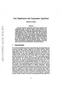


![[PDF] Text Compression Free Ebooks - Google Sites](https://m.moam.info/img/260x300/pdf-text-compression-free-ebooks-google-sites_647763a1097c474b228c051a.jpg)


