Modeling Luminosity-Dependent Galaxy Clustering Through Cosmic ...

Draft version February 5, 2008 Preprint typeset using LATEX style emulateapj v. 6/22/04

MODELING LUMINOSITY-DEPENDENT GALAXY CLUSTERING THROUGH COSMIC TIME Charlie Conroy, Risa H. Wechsler1 , Andrey V. Kravtsov

arXiv:astro-ph/0512234v2 21 Feb 2006

Department of Astronomy and Astrophysics, Kavli Institute for Cosmological Physics, & The Enrico Fermi Institute, The University of Chicago, 5640 S. Ellis Ave., Chicago, IL 60637 Draft version February 5, 2008

ABSTRACT We employ high-resolution dissipationless simulations of the concordance ΛCDM cosmology (Ω0 = 1 − ΩΛ = 0.3, h = 0.7, σ8 = 0.9) to model the observed luminosity dependence and evolution of galaxy clustering through most of the age of the universe, from z ∼ 5 to z ∼ 0. We use a simple, nonparametric model which monotonically relates galaxy luminosities to the maximum circular velocity of dark matter halos (Vmax ) by preserving the observed galaxy luminosity function in order to match the halos in simulations with observed galaxies. The novel feature of the model is the use of the maximum acc circular velocity at the time of accretion, Vmax , for subhalos, the halos located within virial regions of acc larger halos. We argue that for subhalos in dissipationless simulations, Vmax reflects the luminosity and stellar mass of the associated galaxies better than the circular velocity at the epoch of observation, now Vmax . The simulations and our model L−Vmax relation predict the shape, amplitude, and luminosity dependence of the two-point correlation function in excellent agreement with the observed galaxy clustering in the SDSS data at z ∼ 0 and in the DEEP2 samples at z ∼ 1 over the entire probed range of projected separations, 0.1 < rp /(h−1 Mpc) < 10.0. In particular, the small-scale upturn of the correlation function from the power-law form in the SDSS and DEEP2 luminosity-selected samples is reproduced very well. At z ∼ 3 − 5, our predictions also match the observed shape and amplitude of the angular two-point correlation function of Lyman-break galaxies (LBGs) on both large and small scales, including the small-scale upturn. This suggests that, like galaxies in lower redshift samples, the LBGs are fair tracers of the overall halo population and that their luminosity is tightly correlated with the circular velocity (and hence mass) of their dark matter halos. Subject headings: cosmology: theory — dark matter — galaxies: halos — galaxies: evolution — galaxies:clustering — large-scale structure of the universe 1. INTRODUCTION

A generic prediction of high-resolution simulations of hierarchical Cold Dark Matter (CDM) models is that virialized regions of halos are not smooth, but contain subhalos — the bound, self-gravitating dark matter clumps orbiting in the potential of their host halo. The subhalos are the descendants of halos accreted by a given system throughout its evolution, which retain their identity in the face of disruption processes such as tidal heating and dynamical friction. Their presence is in itself a vivid manifestation of the hierarchical build-up of halo mass. In the CDM scenario, luminous galaxies form via cooling and condensation of baryons in the centers of the potential wells of dark matter halos (White & Rees 1978; Fall & Efstathiou 1980; Blumenthal et al. 1984). In the context of galaxy formation, there is little conceptual difference between halos and subhalos, because the latter have also been genuine halos and sites of galaxy formation in the past, before their accretion onto a larger halo. We thus expect that each subhalo of sufficiently large mass should host a luminous galaxy and this is indeed supported by self-consistent cosmological simulations (e.g., Nagai & Kravtsov 2005). The observational counterparts of subhalos are then galaxies in clusters and groups or the satellites around individual galaxies. In this sense, we will use the term halos to refer to both distinct halos (i.e., halos not located within the virial 1

Hubble Fellow

radius of a larger system) and subhalos. Although this general picture is definitely reasonable, it is not clear just how direct the relation between halos and galaxies is. One may argue, for example, that the subhalos can be disrupted much faster than the more tightly bound stellar system they host, leaving behind “orphan” galaxies (Gao et al. 2004; Diemand, Moore, & Stadel 2004). At the same time, properties of surviving subhalos, such as maximum circular velocity and gravitationally bound mass, are subject to strong dynamical evolution as they orbit within the potential of their host halo (e.g., Moore et al. 1996; Klypin et al. 1999; Hayashi et al. 2003; Kravtsov et al. 2004a; Kazantzidis et al. 2004). This makes the relation between subhalo properties and galaxy luminosity ambiguous (Nagai & Kravtsov 2005), because the latter may be less affected by dynamical processes but may evolve due to aging of the stellar populations after ram pressure strips the existing gas and the accretion of new gas is suppressed. The key question that we address in this paper is whether there is a one-to-one correspondence between populations of halos in dissipationless cosmological simulations and galaxies in the observable universe. As a test, we use comparisons of the predicted clustering of halos with the available observational measurements of galaxy clustering from z ∼ 5 to the present. During the last decade, large observational surveys of galaxies both at low and high redshifts have tremendously improved our knowledge of galaxy clustering, its evolution, and the relation between the galaxy and mat-

2

CONROY, WECHSLER & KRAVTSOV

ter distributions. A coherent picture has emerged in which bright galaxies are strongly biased with respect to the matter distribution at high redshifts (Steidel et al. 1998; Giavalisco et al. 1998; Adelberger et al. 2003, 2005; Ouchi et al. 2004b, 2005; Lee et al. 2005; Hamana et al. 2005), and in which the bias decreases with time in such a way that the amplitude of galaxy clustering is only weakly evolving (e.g., Ouchi et al. 2004b), as expected in hierarchical structure formation (Col´ın et al. 1999; Kauffmann et al. 1999). The bias is also in general scaleand luminosity-dependent. Bright (red) galaxies are more strongly clustered than faint (blue) galaxies both in the local universe (Norberg et al. 2002; Zehavi et al. 2004, 2005, and references therein) and in the distant past (Coil et al. 2004, 2005b). A recent development is the detection of a departure from a pure power law in the two-point correlation function of galaxies at z ∼ 0 (Zehavi et al. 2004, 2005). This departure is expected in general because the twopoint correlation function is a sum of two separate contributions: the one-halo term, which arises from pairs of galaxies within a distinct dark matter halo, and the two-halo term, which arises from pairs of galaxies from two different distinct halos (e.g., Cooray & Sheth 2002). The one-halo contribution dominates on small scales, while at scales larger than the size of the largest virialized regions clustering is due to the two-halo term. The two terms are not generically expected to combine so as to give a power-law correlation function. The deviation of the correlation function from a powerlaw was predicted to be even stronger at higher redshifts (Zheng 2004; Kravtsov et al. 2004b), and this has now been convincingly confirmed (Adelberger et al. 2005; Ouchi et al. 2005; Lee et al. 2005; Hamana et al. 2005) using galaxy samples identified with the Lymanbreak technique (Steidel et al. 1996, 1999). Despite impressive advances in the amount and quality of data on the galaxy distribution over a wide range of redshifts, the exact relation between dark matter halos and luminosity- or Lyman-break-selected galaxies is still rather uncertain (e.g., Mo et al. 1999; Kolatt et al. 1999; Wechsler et al. 2001). The most popular attempts to connect the dark halos and luminous galaxies employ semi-analytic modeling (e.g., White & Frenk 1991; Kauffmann et al. 1994; Avila-Reese et al. 1998; Somerville & Primack 1999; Cole et al. 1994, 2000; Croton et al. 2005; Bower et al. 2005), which uses phenomenological recipes for specifying when, where, and how galaxies form within dark matter halos, often in conjunction with high-resolution dissipationless simulations. Another popular approach is to use the halo model (see e.g. Cooray & Sheth 2002, and references therein), which, in its simplest form, specifies the probability distribution for a particular halo of mass M to host a given number of galaxies N with specified properties, such as luminosity, color, etc. More complex halo models include the conditional luminosity function (CLF) approach (Yang et al. 2003; Cooray 2005a,b) which specifies the luminosity function for halos of mass M , and models which connect other features (e.g., Vale & Ostriker 2004; Neyrinck, Hamilton, & Gnedin 2005). While these approaches manage to capture the general observational trends, they usually employ a large number of free parameters, making it difficult to glean

the relevant underlying mechanism(s) responsible for the agreement between the model and data. Most implementations also do not provide a direct constraint on the relation between luminous components of galaxies and dark matter halos. In fact, assumptions are made about this relation in most cases. In this study we use galaxy clustering to address two straightforward issues. First, we question whether current data is consistent with a one-to-one correspondence between luminous galaxies and galaxy-sized dark matter halos in cosmological simulations. Second, we ask whether the observed clustering is consistent with a simple relation between galaxy luminosity and some property of its host halo. In the context of the second question, we investigate which halo properties are most closely related to galaxy luminosity. We show with the currently available data the answer to both of these questions is yes, as we can reproduce luminosity-dependent clustering measurements at different redshifts from z ∼ 5 to z ∼ 0 with a simple, non-parametric model relating galaxy luminosity to the halo circular velocity. Although a number of studies during the last decade have shown that galaxy clustering can be approximately matched by the clustering of dark matter halos in dissipationless simulations (Carlberg 1991; Brainerd & Villumsen 1992, 1994b,a; Col´ın, Carlberg, & Couchman 1997; Wechsler et al. 1998; Col´ın et al. 1999; Kravtsov & Klypin 1999; Kravtsov et al. 2004b; Neyrinck et al. 2004) the size of observational samples did not allow thorough tests of the galaxy-halo relation. For example, Kravtsov et al. (2004b) and Neyrinck et al. (2004) compare the twopoint correlation function of halos and bright galaxies from the SDSS and PSCz surveys, respectively, and find good agreement on scales 0.1 . r/(h−1 Mpc) . 10. However, these studies do not attempt to match the clustering of fainter galaxies. Tasitsiomi et al. (2004) assign luminosities to halos and compute the galaxymass correlation function, finding good agreement for two broad luminosity bins, after a reasonable amount of scatter was introduced into the relation. The current work extends these analyses by comparing results of very high-resolution simulations to the most current measurements of the two-point correlation functions over a wide range of luminosities and redshifts. The large size and wide luminosity range of observational samples allows us to test the relation between galaxy luminosities and properties of their host halos with unprecedented power. The novel feature of the simulation analysis we present is that for each halo and subhalo we track the evolution of its properties, such as mass and maximum circular velocities. As we show below, this is a key piece of information for reasons that are easy to understand. For distinct halos, the current circular velocity is a measure of their potential well built-up during evolution, and can therefore be expected to be tightly correlated with the stellar mass (or more generally the baryonic mass) of the galaxy the halo hosts. The circular velocity of subhalos in dissipationless simulations, on the other hand, is a product of both mass buildup during the period when the halo evolved in isolation and tidal mass loss after the halo starts to orbit within the virialized region of a larger object and experience strong tidal forces (Hayashi et al. 2003; Kravtsov et al.

MODELING GALAXY CLUSTERING THROUGH COSMIC TIME

2. THE SIMULATIONS

The simulations used here were run using the Adaptive Refinement Tree (ART) N -body code (Kravtsov et al. 1997; Kravtsov 1999). The ART code implements successive refinements in both the spatial grid and temporal step in high density environments. These simulations were run in the concordance flat ΛCDM cosmology with Ωm = 0.3 = 1 − ΩΛ , h = 0.7, where Ωm and ΩΛ are the present-day matter and vacuum densities in units of the critical density, and h is the Hubble parameter in units of 100 km s−1 Mpc−1 . The power spectra used to generate the initial conditions for the simulations were determined from a direct Boltzmann code calculation (courtesy of Wayne Hu). We use a power spectrum normalization of σ8 = 0.90, where σ8 is the rms fluctuation in spheres of 8h−1 Mpc comoving radius. To study the clustering properties of dark matter halos over a range of scales, we consider two simulations of the above cosmology The first simulation, L80, followed the evolution of 5123 particles in a 80h−1 Mpc box. The L80 simulation has a particle mass of mp = 3.16×108 h−1 M⊙ and peak force resolution hpeak = 1.2 h−1 kpc. This is the simulation to which we make most comparisons with observations. The second simulation we consider is

100

z=0 z=1 z=3 z=4

n(>Vacc max )

10−1 10−2 10−3 10−4 10−5

(nsub/ntot)(>Vacc max )

2004a; Kazantzidis et al. 2004). The stellar component of the galaxies, which should be more tightly bound than halo dark matter, should not be significantly affected by tidal forces and can stabilize the mass distribution (and hence Vmax ) in the inner regions. We can therefore expect that luminosity and stellar mass of galaxies hosted by halos in dissipationless simulations should be correacc lated with the subhalo mass or circular velocity, Vmax , at the epoch of accretion, rather than with its current value. This is borne out by cosmological simulations, which include gas dynamics, cooling, and star formation (Nagai & Kravtsov 2005) who show that selection using acc Vmax results in subhalo properties similar to the selection based on stellar mass of galaxies subhalos host. One can therefore argue that a reasonable approach is to relate galaxy luminosity to the current halo circular velocity for distinct halos and to the circular velocity at accretion for subhalos. The main result of this study is that this simple model reproduces the luminosity-dependence of galaxy clustering at different epochs with remarkable, and perhaps surprising, accuracy. We note that Vale & Ostriker (2005) have recently presented and used a semi-analytic model for subhalos, which employs a similar approach to luminosity assignment, except that they use the total bound halo mass instead of circular velocity. The paper is organized as follows. In §2 we briefly describe the simulations, halo finding algorithm, and the method for tracking the evolution of halos. §3 details our method for relating halos to galaxies, and elaboacc rates upon our motivation for using Vmax as the basis for the luminosity assignment for subhalos. In §4 we compare observational clustering results over the redshift interval 0 < z < 5 to the clustering of halos in dissipationless ΛCDM simulations. The halo occupation distribution implied by this model is described in §5. In §6 we discuss the implications of our results and in §7 we summarize our main conclusions. Throughout this paper we assume a ΛCDM cosmology with (Ωm , ΩΛ , h, σ8 ) = (0.3, 0.7, 0.7, 0.9).

3

0.10

0.01 100

1000 −1 Vacc max (km s )

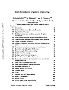
Fig. 1.— Top panel: Cumulative velocity function for all halos identified in the L80 simulation at various redshifts, in units of 3 h Mpc−3 . Bottom panel: Fraction of subhalos as a function of redshift and maximum circular velocity at the time of accretion, acc . We truncate the curves where N Vmax sub < 10 because in that regime poisson noise washes away any useful information. The arrow delimits our nominal completeness limit.

denoted L120 and was run with 5123 particles in a 120 h−1 Mpc box, resulting in a particle mass of mp = 1.07 × 109 h−1 M⊙ and peak force resolution hpeak = 1.8 h−1 kpc. This simulation thus has a larger particle mass and somewhat lower spatial resolution compared to the L80 run. We use this simulation to obtain better statistics for the correlation function of rare (i.e., massive) objects. 2.1. Halo Identification, Classification, and

Construction of Merger Trees Our analysis requires detailed dynamical knowledge of not only distinct halos, i.e. halos with centers that do not lie within any larger virialized system, but also subhalos which are located within the virial radii of larger systems. Note that the term “halo” (e.g., the halo occupation distribution) usually refers to what we call distinct halos in this work. We identify distinct halos and the subhalos within them using a variant of the Bound Density Maxima (BDM) halo finding algorithm (Klypin et al. 1999). Details of the algorithm and parameters used can be found in Kravtsov et al. (2004b); we briefly summarize the main steps here. All particles are assigned a density using the smooth algorithm2 which uses a symmetric SPH smoothing kernel on the 32 nearest neighbors. Starting with the highest overdensity particle, we surround each potential center by a sphere of radius rfind = 50h−1 kpc and exclude all particles within this sphere from further search. Hence no two halos can be separated by less than 2 To calculate the density we use the publicly available code smooth: http://www-hpcc.astro.washington.edu/tools/ tools.html

CONROY, WECHSLER & KRAVTSOV

rfind . We then construct density, circular velocity, and velocity dispersion profiles around each center, iteratively removing unbound particles as described in Klypin et al. (1999). Once unbound particles havep been removed, we measure quantities such as Vmax = GM (< r)/r|max , the maximum circular velocity of the halo. For each distinct halo we calculate the virial radius, defined as the radius enclosing overdensity of 180 with respect to the mean density of the Universe at the epoch of the output. We use this virial radius to classify objects into distinct halos and subhalos. The halo catalog is complete for halos with more than 50 particles which corresponds, for the L80 simulations, to a minimum halo mass of 1.6 × 1010 h−1 M⊙ . acc For subhalos we also tabulate Vmax , the maximum circular velocity at the time when a subhalo falls into a distinct halo. In order to tabulate this quantity we rely on merger trees generated for these simulations, which track the histories of both distinct halos and subhalos. A detailed description of the merger tree construction is given in Allgood (2005). The merger trees we use here follow halo evolution through 48 timesteps between z = 7 and the present for the L80 box and 89 timesteps for the L120 box. For each subhalo, we use the merger trees to step back in time until the subhalo is no longer identified acc as belonging to a larger system. We then define Vmax to be Vmax of the subhalo at that time. In the top panel of Figure 1 we show the cumulative velocity function for all identified halos from z = 4 to 0. acc and n, as This figure quantifies the relation between Vmax we will use these two quantities interchangeably to define our halo samples throughout the paper. In the bottom panel we show the corresponding cumulative fraction of subhalos as a function of time. The figure shows that the subhalo fraction is a weak function of circular velocity at all epochs. There is a weak trend for a smaller acc subhalo fraction among halos with larger Vmax . There is a stronger trend of increasing subhalo fraction with decreasing redshift.

3. CONNECTING GALAXIES TO HALOS

In this section we motivate and describe our model for associating galaxies with dark matter halos. We make this connection by relating galaxy luminosity and a physical property of dark matter halos, for which we choose now acc Vmax for distinct halos and Vmax for subhalos. As disacc cussed above, for subhalos Vmax denotes the maximum circular velocity at the time the subhalo was accreted. The maximum of the circular velocity profile, Vmax , is a measure of the depth of the halo potential well and is expected to correlate strongly with stellar mass of the galaxies, as implied by the Tully-Fisher and FaberJackson relations. At the same time, the definition of Vmax in simulations is unambiguous both for distinct halos and subhalos, which is not the case for the total mass, as different operational definitions are used by different authors. It should be noted that Vmax used here will not correspond directly to Vmax observed in, for example, the Tully-Fisher relation because dissipationless simulations do not take into account the effect of baryon condensation on Vmax (e.g., Blumenthal et al. 1986). acc The use of Vmax for subhalos is the novel feature

103 1.0E−3

6.0E−3

1.5E−2

2.8E−2

102 Vacc Vnow

ωp(rp)

4

101

102

101 0.1

1.0

0.1 rp (h−1 Mpc)

1.0

10.0

Fig. 2.— Projected two-point correlation function at z ∼ 0 acc (solid lines) versus comparing the effects of selecting on Vmax now Vmax (dashed lines) at four different number density thresholds (labeled in the top right corner, in units of h3 Mpc−3 ). While there is a slight increase in the correlation function on large scales acc rather than V now , the difference is much stronger when using Vmax max acc and V now is due to on small scales. The difference between Vmax max the tidal stripping of subhalos which have fallen into larger systems, hence correlation functions will be most strongly effected on small scales.

of our model3 . As we discussed in the introduction, the motivation for this is fairly straightforward. While Vmax decreases due to tidal stripping as a halo falls through a larger halo (Hayashi et al. 2003; Kravtsov et al. 2004a), one can expect that the stellar component of galaxies within these halos will not be affected appreciably since stars are concentrated near the bottom of the halo potential well and are more tightly bound (e.g., Nagai & Kravtsov 2005). Hence we argue that, for galaxies associated with subhalos, luminosity acc now than the Vmax should correlate more strongly with Vmax affected by dynamical evolution. Therefore, throughout the rest of the paper, unless explicitly stated otherwise, the maximum circular velocity, Vmax , will be assumed to mean:  acc Vmax , subhalos Vmax = (1) now Vmax , distinct halos Although it is not clear how accurate this assumption is in detail, we show that it provides a considerably better match to observed galaxy clustering compared to the now uniform selection using Vmax for both subhalos and distinct halos. Note also that the use of circular velocities before accretion can also help explain the abundance of faint dwarf galaxies in the Local Group (Kravtsov et al. 2004a). In order to assign luminosities, we assume a monotonic relation between galaxy luminosity and Vmax and 3 As we prepared this paper for publication, Vale & Ostriker (2005) submitted a paper in which they employ a semi-analytic model for subhalos and a similar approach to luminosity assignment, except that they use the total bound halo mass instead of circular velocity.

MODELING GALAXY CLUSTERING THROUGH COSMIC TIME require that the L−Vmax relation preserves the galaxy luminosity function (LF). Specifically, we use the following equation:

104

ng (> Li ) = nh (> Vmax ,i )

(2)

102

where ng and nh are the number density of galaxies and halos, respectively. We stress again, that Vmax in the acc above expression is equal to Vmax for subhalos and to now Vmax for distinct halos (for which the accretion epoch is undefined). For each Li we find the corresponding Vmax,i such that the above relation is satisfied. The main assumption is therefore that there is a monotonic relation between galaxy luminosity and Vmax . The model makes no further assumptions and is completely nonparametric. This should be kept in mind when we compare predictions of this model to observed galaxy clustering. Note that we do not take any possible scatter in the L−Vmax relation into account in this model. With the L−Vmax relation in hand, comparing observational clustering statistics to the model predictions is straightforward: we simply compute the desired statistic for the halos with assigned luminosities corresponding to the observed sample luminosity range. This method does not currently treat other galaxy properties such as color, although it could conceivably be extended to include such properties. We have not included the possibility of “orphaned galaxies”, i.e. galaxies without any associated subhalos. We discuss the issue of orphans in detail in §6. Figure 2 shows the effect that selection of halos using acc now Vmax rather than Vmax for subhalos has on the projected two-point correlation function ωp for different number densities, at z = 0. As expected, the effect is most significant on small scales, where the subhalo contribution now acc is and Vmax dominates, and the difference between Vmax greatest. In Figure 3 we show the effect of selecting halos acc now according to Vmax and Vmax on the galaxy-mass crosscorrelation function, ξgm . The small bump in the samacc ple selected using Vmax in the top panel is due to the fact acc samples in general have more satellites than that Vmax now samples, and the satellite contribution to ξgm peaks Vmax near rp = 0.5 h−1 Mpc. The “bump” is smaller in the lower panel, where the Vmax threshold is much higher, because the number of satellites is nearly the same between acc now selected samples in this case. and Vmax the Vmax At higher redshifts the differences between samples acc now selected using Vmax and Vmax are small.4 Figure 4 acc shows the projected correlation function for the Vmax now and Vmax -selected samples at four redshifts. The samples are constructed to have a fixed number density n = 1.5 × 10−2 h3 Mpc3 . The situation is similar for other number densities. Already by z ∼ 1 the effect of selection is quite small. The difference on small scales for the z ∼ 3 and z ∼ 4 samples is not statistically significant.5

10−1

4 Note that the designation “now” refers to the time of observation, not to z = 0. 5 Note that at high z the correlation function at the smallest now -selected samples, which scales is somewhat higher for the Vmax seems counter-intuitive. We believe that this is a small artefact of the halo finding algorithm. At higher redshifts, the halos are smaller and subhalos are typically at smaller distances from the host center. At small radii the removal of unbound particles is more difficult as the halos are located near the bottom of the po-

V>150

103

ξgm

100

5

Vacc Vnow

10−1 V>280

103 102 10−1 100 10−1 0.1

1.0 rp (h−1 Mpc)

10.0

Fig. 3.— Comparison of the galaxy-mass cross-correlation funcacc (solid lines) and V now (dashed tion for halos selected using Vmax max lines) at two different circular velocity thresholds (labeled in the top right corner of each panel, in units of km s−1 ).

z=0

z=1

z=3

z=4

ωp(rp)

100

10

Vacc Vnow

100

10 0.1

1.0

0.1 rp (h−1 Mpc)

1.0

10.0

Fig. 4.— Comparison of the projected two-point correlation funcacc (solid lines) and V now (dashed tion for halos selected using Vmax max lines) at four different redshifts, for a fixed number density, n = 1.5 × 10−2 h3 Mpc−3 . This figure clearly shows that, while using acc over V now results in a large difference at low redshift, it has Vmax max very little impact at higher redshifts. The trend is similar for a wide range of number densities.

now in such cases can be overestimated tential well. The value of Vmax producing a boost in the number of subhalos above a given threshold value, and boosting the correlation function somewhat. Note, however, that the effect is small and the difference between correnow - and V acc -selected samples is less than lation functions for Vmax max 2σ.

6

CONROY, WECHSLER & KRAVTSOV

We believe that this effect can be attributed to the distribution of accretion times for subhalos at each redshift: at low redshift, subhalos have a wide distribution of accretion times, and hence a large number of subhalos have had time to experience significant tidal stripping, while at higher redshifts the distribution of accretion times rises sharply near the epoch of observations. This is because both the accretion and disruption rates are high at high redshifts. The accreted halos do not survive for a prolonged period of time, so that at each high-z epoch most of identified subhalos are recently accreted objects, which are yet to experience significant tidal mass loss. acc Since we are only computing Vmax for subhalos which have survived to the current epoch, one may worry that we are neglecting a significant population of subhalos acc with a sizeable Vmax that are not present in the halo catalog at the current epoch. Of such a population there can only be two fates: either the object was at some point physically disrupted or it has simply fallen below the resolution limit. We have used the merger trees to find all subhalos which have ever fallen into a distinct acc halo and have tabulated their Vmax and the ratio in mass between the subhalo and distinct halo, at the time of acc accretion. For a wide range in Vmax thresholds, the distribution of mass ratios is strongly peaked between 0.1 and 1.0. This implies that dynamical friction has caused the subhalo to merge with the distinct halo on the order of a dynamical time, and suggests that the majority of these subhalos have in fact physically merged and should not have survived. The absence of such missing subhalos also implies that in our simulations there should be no “orphan” galaxies (Gao et al. 2004, see § 6 for further discussion of this issue). 4. GALAXY CLUSTERING FROM Z ∼ 5 TO THE PRESENT

In this section we compare clustering statistics of halos to recent observations of the galaxy two-point correlation function over the redshift interval 0 . z . 5. The observed clustering statistics we compare to are ωp (rp ), the projected two-point correlation function, and ω(θ), the angular two-point correlation function. We estimate ωp by integrating the real space, three-dimensional correlation function, ξ(r), computed in the simulation, along the line of sight: Z ∞ q ξ( rp2 + rk2 )drk , ωp (rp ) = 2 (3) 0

where the comoving distance r has been decomposed into perpendicular (rp ) and parallel to the line-of-sight (rk ) components. In practice, the integration in Eqn. 3 is truncated at some finite scale: we truncate at 40h−1 Mpc for SDSS galaxies (§4.1) and 20h−1 Mpc for DEEP2 galaxies (§4.2), as is done in the data. Since the simulation box size is only 80h−1 Mpc, the measurement of ξ(r) is not reliable for r & 0.1Lbox ∼ 8h−1 Mpc. To extrapolate ξ(r) to larger scales, we use ξm (r), the two-point correlation function of dark matter 6 , multiplied by the linear bias of ξ(r) measured over 4 < r/(h−1 Mpc)< 8. 6 We derive the dark matter correlation function from the power spectrum provided by the publicly available code of Smith et al. (2003), which is more accurate than the popular Peacock and Dodds prescription.

Generating ω(θ) from ξ(r) without assuming ξ(r) to be a power law is somewhat more involved. With knowledge of the redshift distribution, N (z), of the sample, ω(θ) can be derived via the Limber transformation: p R∞ R∞ 2 2 2 0 dzN (z) −∞ dxξ( [Dm (z)θ] + x )/RH (z) R∞ ω(θ) = [ 0 dzN (z)]2 (4) where Dm (z) is the proper motion distance and RH (z) is the Hubble radius at redshift z. As for ωp , the integral over ξ(r) is in practice truncated at a finite scale; we integrate to 50 h−1 Mpc and note that the resulting ω(θ) is not sensitive to this particular truncation scale. 4.1. Clustering at z ∼ 0

The SDSS (York et al. 2000; Abazajian et al. 2004) is a large photometric and spectroscopic survey of the local Universe. Zehavi et al. (2005) have measured the luminosity and color dependence of wp (rp ) for ∼ 200, 000 SDSS galaxies over ≈ 2500 deg2 with z < 0.15. As mentioned in §3, assigning Vmax to galaxy luminosity while preserving the observed luminosity function (LF) results in a unique L−Vmax relation. In order to make the assignment we use the SDSS luminosity function presented in Blanton et al. (2003), with Schechter (1976) parameters in the r-band Mr∗ − 5logh = −20.5, α = −1.05, and φ∗ = 1.5 × 10−2 h−3 Mpc3 . It is then straightforward to compare the observed luminosity dependence of both the small and large scale clustering of SDSS galaxies to our model. The results for luminosity threshold samples (L > Lth ) are shown in the left panel of Figure 5, where we compare the Zehavi et al. (2005) results to the clustering of halos corresponding to the range of galaxy luminosities in each sample. For the three halo samples with n = 6 × 10−3 h3 Mpc−3 , n = 1.5 × 10−2 h3 Mpc−3 and n = 2.8 × 10−2 h3 Mpc−3 we use the L80 simulation, while for the halo sample with n = 1.1 × 10−3 h3 Mpc−3 we use the L120 simulation in order to improve statistics. See Table 1 for details of the SDSS samples used here. The agreement is excellent over all scales. We find similar agreement when wp (rp ) is measured in differential, rather than integral, luminosity bins. It is critical to realize that the agreement on scales rp . 1h−1 Mpc is due to our luminosity acc assignment scheme using Vmax . The luminosity assigned now for subhalos would result in a significant using Vmax under-prediction of amplitude of ωp at rp . 1h−1 Mpc, especially for fainter samples (see Figure 2). The halo occupation distribution (HOD) specifies the distribution of the number of galaxies within a (distinct) halo of mass M , P (N |M ). It has become a popular tool for interpreting galaxy clustering (Jing et al. 1998; Seljak 2000; Scoccimarro et al. 2001; Bullock, Wechsler, & Somerville 2002; Yan, Madgwick, & White 2003; Berlind et al. 2003; Zehavi et al. 2005; Kravtsov et al. 2004b; Zheng 2004; Abazajian et al. 2005; Tinker et al. 2005), which requires that the first two moments of P (N |M ) be specified to calculate two-point clustering. In the right panel of Figure 5 we show the first moment of this distribution, the average number of galaxies within a (distinct) halo of mass M , hN (M )i, for the four halo samples which correspond to the four luminosity threshold SDSS samples in the left panels. As expected,

MODELING GALAXY CLUSTERING THROUGH COSMIC TIME 103

Mr−5log(h)