Modeling particle transport and aggregation in a ... - Stanford University

WATER RESOURCES RESEARCH, VOL. 36, NO. 8, PAGES 2249 –2261, AUGUST 2000

Modeling particle transport and aggregation in a quiescent aqueous environment using the residence-time scheme J. Gabriel Perigault, James O. Leckie, and Peter K. Kitanidis Department of Civil and Environmental Engineering, Stanford University, Stanford, California

Abstract. Suspended particles are a ubiquitous component of aqueous environments and are found over broad ranges of size and density. Particle transport and fate have an important role in the regulation of contaminants and nutrients in natural settings. The mechanisms that control the transport and size of particulate material in solution also play a fundamental role in the successful operation of engineered systems, such as sedimentation ponds and flocculation tanks, as well as flotation and filtering reactors. Adequate modeling of particle transport and aggregation is required for better understanding and prediction of the effects of particulate material in natural aqueous systems, as well as for designing efficient physicochemical processes to deal with suspended solids. In this paper we illustrate how numerical diffusion produced by the use of first-order finite difference schemes can introduce significant errors in the modeling of particle settling in quiescent systems and how this error is compounded when aggregation is considered. To model settling without introducing numerical diffusion, while preserving numerical efficiency, we propose the residence-time scheme, a simple numerical scheme based on the residence time of each size fraction in the elements of the spatial discretization. For the solution of the settling-aggregation equation the alternatingoperator-splitting technique (AOST) is used. The inherent modularity and simplicity of AOST allows smooth incorporation of additional particle transport mechanisms such as mixing, advection, etc.

1.

Introduction

An increasing amount of scientific evidence indicates that microscopic particles, because of their ubiquity, large surface area, and varying residence times, play a key role in the transport and regulation of contaminants and nutrients in surface and subsurface natural aqueous systems [McCarthy and Zachara, 1989; Tiller and O’Melia, 1993]. The hydrodynamic, chemical, and biological conditions of the environment in which the particles are suspended determine the extent of this role [Ali et al., 1984; Boehm and Grant, 1998]. Adequate modeling of particle transport and aggregation is a necessary component of any realistic attempt to predict the fate of contaminants and nutrients. Engineering processes, such as sedimentation, flocculation, and filtering, rely on particle-particle interactions [Valioulis and List, 1984; Wilson and Barfield, 1985] and would also benefit from improvements in the predictive capabilities of models dealing with particle transport and aggregation. The lack of adequate mathematical schemes to solve the expressions used to describe the particle transport and aggregation phenomena remains an important problem that limits our ability to predict the behavior of particulate material in suspension. Usually the set of equations used to describe particle transport and aggregation do not have general analytical solutions and must be solved numerically. However, the domain discretization required for these numerical schemes can introduce artifacts such as numerical diffusion and numerical instabilities. Finer discretization reduces these problems but Copyright 2000 by the American Geophysical Union. Paper number 2000WR900088. 0043-1397/00/2000WR900088$09.00

increases computational time to the point that, in some cases, the problem becomes numerically intractable. This work analyzes numerical methods for particle settling and aggregation in systems under quiescent hydrodynamic conditions. Perfect quiescence is not found in natural or engineered systems. However, it is often the case that the settling velocity of dense (density ⬎2 g mL⫺1), large particles (diameter ⬎15 ␮m) is significantly larger than the fluid movement. Natural systems, such as lake hypolimnions, and engineered systems, such as settling tanks and sedimentation ponds, can then be treated as quiescent, where settling controls particle transport. First-order finite difference schemes for solving particle settling [Lawler et al., 1980; Valioulis and List, 1984; Wilson and Barfield, 1985; Gardner, 1995] are prevalent in practice. The limitations of such schemes for solving fluid advection have been the focus of great attention [Warming et al., 1973; Tannehill, 1988; Islam and Chaudhry, 1997] but not in the context of solving particle settling and aggregation. In this study, we start by analyzing some artifacts introduced by the use of first-order finite difference numerical schemes in the modeling of particle settling and show the effect of these artifacts when particle aggregation is considered. A new numerical scheme is presented, the residence-time scheme (RTS), to adequately model particle settling. Then, we apply the alternating-operator-splitting technique (AOST), a methodology widely used for solving transport-reaction aqueous systems [Valocchi and Malmstead, 1992; Kaluarachchi and Morshed, 1995a, b], for solving the equations governing particle transport and aggregation. We discuss why AOST is a computationally efficient and flexible methodology compared with more traditional numerical frameworks used to model the fate of microscopic particles in aqueous systems.

2249

2250

PERIGAULT ET AL.: MODELING PARTICLE TRANSPORT AND AGGREGATION

Table 1. Collision Frequency Functions for Various Mechanisms Collision Mechanism

Collision Frequency Function

Brownian

␤v,v* Brownian ⫽

Fluid shear

␤v,v* shear ⫽

Differential settling

␤v,v* settling ⫽

冉 冊冋冉 冊 冉 冊 册 2kb T 3␮

1/3

1 v

⫹

1 v*

Source

1/3

Smoluchowski [1917]

共v1/3 ⫹ v*1/3 兲

G 1/3 共v ⫹ v*1/3 兲3 ␲

冉冊 6 ␲

1/3

Smoluchowski [1917]

g 共␳ ⫺ ␳fluid兲共v1/3 ⫹ v*1/3 兲3 兩v1/3 ⫺ v*1/3 兩 12␮ solid

Friedlander [1977]

Here k b is the Boltzman constant, T is the temperature, ␮ is the fluid’s dynamic viscosity, v and v* are the volumes of the colliding particles, G is the mean velocity gradient, g is the gravitational acceleration, and ␳solid and ␳fluid are the particle’s and fluid’s densities, respectively.

2.

Particle Transport and Aggregation Theory

Particle transport is due to fluid advection, fluid mixing, and particle settling. Typically, more than one mechanism is present, albeit generally one may dominate the overall process. The change in size distribution is due to aggregation/ disaggregation processes. Where turbulence is low and biological and chemical perturbations are absent, particle disaggregation is negligible for sizes under 250 ␮m [Parker et al., 1972]. Particle aggregation is the result of collisions generated because of the relative motion between the particles. The causes of this relative motion are classified in three categories: Brownian diffusion, fluid shear, and differential settling. Collision frequency functions for each of these mechanisms quantify the rate of interparticle binary collisions. As a result of interparticle forces such as electrostatic repulsion, hydration forces, steric effects, and other factors, not every collision results in aggregation [Verwey and Overbeek, 1948; O’Melia and Bowman, 1984; Liang, 1988; Gardner, 1995]. In colloidal science vernacular the collision efficiency for a homogeneous dispersion ␣ is defined as the ratio of the collisions that result in aggregation divided by the total number of collisions. Equation (1) is the one-dimensional form of the particle transport aggregation (PTA) equation and represents the change of the size distribution function of particles of volume v over time, as a result of particle transport and particle collisions [Smoluchowski, 1917; Lawler et al., 1980; Valioulis and List, 1984]: ⭸n共v兲 ⫽ ⭸t

再冕 1 2

⫺

v

␣ 共v*, v ⫺ v*兲 ␤ 共v*, v ⫺ v*兲n共v*兲n共v ⫺ v*兲 dv*

0

冕

⬁

⫺

冎 冉 冊

␣ 共v*, v兲 ␤ 共v*, v兲n共v*兲n共v兲 dv*

0

⭸ ⭸W v n共v兲 ⭸Q zn共v兲 ⫺ ⫹ ⭸z ⭸z ⭸z

␧z

⭸n共v兲 . ⭸z

(1)

The first term on the right-hand side of (1) (between braces) represents aggregation (Smoluchowski equation), the second term represents settling, the third term represents advection, and the fourth term represents mixing. Here n(v) is the particle size distribution function in terms of particle volume (v). The terms ␣ (v*, v ⫺ v*) and ␤ (v*, v ⫺ v*) are the collision efficiency and the total collision frequency function between a particle of volume v* and a particle of volume v ⫺ v*, respectively. W v is the particle’s settling velocity, Q z is the

vertical fluid velocity, and ␧ z is the vertical mixing (or dispersion) coefficient. The positive direction of axis z is downward. Table 1 lists collision frequency functions resulting from Brownian diffusion, laminar shear, and differential settling mechanisms. The main assumptions of this approach are the following: 1. The volume of solid particles is conserved during agglomeration, and all aggregates are spheres (coalesced-sphere assumption in collision frequency functions). 2. Particles approach one another on rectilinear paths, and the path of one particle is not affected by the presence of other particles. 3. Collision frequency functions from different mechanisms are assumed to be additive:

␤ 共v, v*兲 ⫽ ␤ 共v, v*兲 Brownian ⫹ ␤ 共v, v*兲 shear ⫹ ␤ 共v, v*兲 setting. 4. Particle collisions are binary (no more than two particles participate in each collision). 5. Particles obey Stokes’ settling velocity expression [McGauhey, 1956]: Wv ⫽

gd v2共 ␳ solid ⫺ ␳ fluid兲 , 18 ␮

(2)

where d v is the diameter of a particle of volume v. 6. Breakup or dissociation of aggregates due to fluid shear or other processes does not occur. 7. Only vertical transport is considered, and no lateral losses occur. The collision frequency functions provided in Table 1 and the settling velocity equation (equation (2)) are simplified expressions. More complex mathematical relations that consider interparticle hydrodynamic effects and forces [Spielman, 1970; Davis, 1984; Han and Lawler, 1991, 1992] and the nonspherical (fractal) nature of particle aggregates [Jiang and Logan, 1991; Johnson and Logan, 1996; Grant et al., 1996; Li and Logan, 1997a, b] have been proposed.

3.

Traditional Modeling Approach

Consider the particular case of a one-dimensional quiescent aqueous environment in which the main mechanism of particle transport is particle settling and collision efficiencies equal unity. Under these conditions the transport due to mixing and advection can be neglected leading to a simplified version of the PTA equation:

PERIGAULT ET AL.: MODELING PARTICLE TRANSPORT AND AGGREGATION

2251

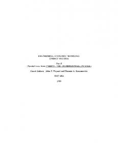
Figure 1. Schematic of discretization used for idealized settling reactor. ⭸n共v兲 ⫽ ⭸t

再冕 1 2

⫺

v

␣ 共v*, v ⫺ v*兲 ␤ 共v*, v ⫺ v*兲n共v*兲n共v ⫺ v*兲 dv*

0

冕

冎

⬁

␣ 共v*, v兲 ␤ 共v*, v兲n共v*兲n共v兲 dv* ⫺

0

⭸W v n共v兲 . ⭸z (3)

There is no known general analytical solution for the PTA equation. Researchers have solved this equation numerically using finite difference schemes [Lawler et al., 1980; Valioulis and List, 1984; Gardner, 1995]. Frequently, (3) has been discretized by dividing the particle population into a finite number of size fractions (NS) and by dividing the region of interest into a finite number of compartments (NC). Figure 1 illustrates the idealized settling tank. The terms that account for the generation and destruction of particles (Smoluchowski equation) and settling could yield stiff systems of equations [Valioulis and List, 1984]. Stiff systems occur when some components of the equations vary much more rapidly than others. To ensure stability, while preserving accuracy and numerical efficiency, schemes suited for solving stiff systems of equations must be used [Press et al., 1992]. The settling term has often been solved by means of firstorder finite differences [Lawler et al., 1980; Valioulis and List, 1984; Wilson and Barfield, 1985; Gardner, 1995]. The resulting discretized equation, assuming compartments of constant depth and settling velocities independent of depth, is ⭸n m,k 1 ⫽ ⭸t 2 ⫺

冘

m⫺1

冘 NS

␤ i,m⫺i,kn i,kn m⫺i,k ⫺ n m,k

i⫽1

Wm 共n m,k ⫺ n m,k⫺1兲. ⌬z

␤ i,m,kn i,k

i

(4)

In this equation, n m,k is the number concentration of particles of size fraction m in compartment k. ⌬z is the vertical length of compartment k (compartment k contains particles within the (k ⫺ 1)⌬z to k⌬z vertical range). The term ␤ i, j,k is the total collision frequency function between a particle of size fraction i and a particle of size fraction j in compartment k. W m is the settling velocity of a particle of size fraction m. Unfortunately, the first-order discretization used for the settling term in (4) introduces numerical diffusion (i.e., artificial diffusion). In the presence of aggregation the error introduced gets compounded when collisions between particle fractions affected by this phenomenon take place. We will explore in more detail the first-order discretization of the settling term in order to understand some of its shortcomings. This scheme, known as the upwind or upstream scheme [Tannehill, 1988; Islam and Chaudhry, 1997], is an explicit first-order finite difference method that employs a forward difference for the time derivative and a backward difference for the space derivative. Applying this methodology to the differential settling component of the PTA equation, we get 共t⫹⌬t兲 共t兲 共t兲 共t兲 n m,k ⫽ n m,k ⫺ C m共n m,k ⫺ n m,k⫺1 兲,

(5)

where C m:Courant number ⫽

W m⌬t . ⌬z

(6)

This method is stable for 0 ⱕ C m ⱕ 1 [Tannehill, 1988; Islam and Chaudhry, 1997]. Although simple, this methodology is of limited use because it introduces numerical diffusion resulting from its truncation error [Islam and Chaudhry, 1997], as we will explain next. If all the concentrations used in (5) are calculated using Taylor’s series, the following equations will be derived:

2252

PERIGAULT ET AL.: MODELING PARTICLE TRANSPORT AND AGGREGATION

共t⫹⌬t兲 共t兲 n m,k ⫺ n m,k ⫽

1 ⭸ 2n m 2 ⭸n m ⌬t ⫹ 0共⌬t 3兲, ⌬t ⫹ ⭸t 2 ⭸t 2

共t兲 共t兲 n m,k⫺1 ⫺ n m,k ⫽⫺

(7)

⭸n m 1 ⭸ 2n m ⌬z 2 ⫹ 0共⌬z 3兲, ⌬z ⫹ ⭸z 2 ⭸ z2

(8)

(t) where n m means n m,k . Additionally, in the absence of aggregation and for spatially uniform W m , from (3),

⭸ 2n m ⭸ 2 ⫽ ⫺W m ⭸t ⭸t

冉 冊

⭸n m ⭸ ⫽ ⫺W m ⭸z ⭸z

冉 冊

⭸n m ⭸ 2n m 2 ⫽ Wm . ⭸t ⭸ z2 (9)

Substituting (7), (8), and (9) into (5), we get ⭸n m ⭸ 2n m ⭸n m , ⫽ ⫺W m ⫹ Dm ⭸t ⭸z ⭸ z2

(10)

where D m is the numerical diffusion coefficient: Dm ⫽

W m⌬z 共W m兲 2⌬t W m⌬z ⫺ ⫽ 共1 ⫺ C m兲. 2 2 2

(11)

Thus the truncation error not only introduces a fictitious diffusion or mixing, but it produces a different diffusion coefficient for each particle size. If ⌬z and W m are constants, the range of possible D m will be constrained by the stability restrictions on C m : 0 ⱕ Dm ⬍

W m⌬z . 2

(12)

Interestingly, smaller time increments increase the magnitude of the numerical diffusion coefficient. For the case of a polydisperse system of particles the maximum time increment that preserves the algorithm stability is ⌬t ⫽ ⌬z/W max size,

(13)

where W max size is the settling velocity of the largest particle size considered. For this time step the numerical diffusion for the largest particle size vanishes. Substituting (13) into (11), Dm ⫽

W m⌬z 共W m兲 2⌬z . ⫺ 2 2W max size

The operator-splitting technique (OST) has been widely used for the solution of the advection-dispersion-reaction equations [Valocchi and Malmstead, 1992; Kaluarachchi and Morshed, 1995a, b]. As noted by Valocci and Malmstead [1992], the use of OST is advantageous because it allows the use of the numerical scheme best suited for each process. OST also improves programming modularity and is computationally efficient. Equation (3) is a nonlinear partial differential equation that can be converted to a linear partial differential equation plus a nonlinear ordinary differential equation by splitting the transport and aggregation terms. Additionally, usually the transport and aggregation processes have different timescales. By splitting the transport and aggregation terms, the efficiency of the algorithm is improved because different time steps can be used for solving each process. However, the splitting of a simultaneous process introduces an inherent error independent of the spatial and size discretization. This error has been referred to as the time-lag error [Kaluarachchi and Morshed, 1995a]. One way to minimize this inherent error is to adopt a technique known as alternatingoperator-splitting technique (AOST) [Valocchi and Malmstead, 1992; Kaluarachchi and Morshed, 1995a, b]. The basic idea behind AOST algorithms is to alternate the order in which the operators of the transport and reaction terms are solved for each time step. The use of this technique can reduce the error by an order of magnitude [Kaluarachchi and Morshed, 1995b]. To overcome the numerical diffusion problems and numerical instabilities produced by finite difference schemes, a methodology based on residence times of the different size fractions is introduced. We have termed it the residence-time scheme (RTS). This scheme is a subset of the upstream or upwind scheme for the case of Courant number equal to one and corresponds to the exact solution of the settling term. Since different particles have different settling velocities, the former condition will be satisfied at different time steps. Particles of a given size fraction (m) in a given compartment (k) are allowed to settle to the next compartment (k ⫹ 1) only when their time in that compartment has reached their residence time. The residence time (␶m) of particles of size fraction m in a compartment of length ⌬z is defined as

(14)

Higher-order finite difference schemes such as the Warming-Kuttler-Lomax [Warming et al., 1973; Tannehill, 1988], a third-order predictor-corrector method, can be used to minimize numerical diffusion. However, they increase computational cost, and for sharp fronts they produce artificial oscillations (sometimes predicting unfeasible outcomes, such as negative concentrations) without totally eliminating numerical diffusion.

␶ m ⫽ ⌬z/W m.

A schematic algorithm of the mathematical formulation of RTS is presented in the appendix. The advantages of RTS include the elimination of the artificial diffusion and low computational cost. The use of RTS for the solution of the settling term exemplifies the benefits of using AOST. The flexibility of AOST allows us to use the numerical scheme that is best suited for settling transport.

5. 4.

Proposed Modeling Strategy

The PTA equation for a quiescent system (equation (3)) describes two simultaneous processes: particle settling (transport) and particle aggregation. Particle aggregation acts as a source/sink term for each size fraction. In other words, the aggregation of particles changes the particle size distribution, increasing some size fractions and decreasing others. With this in mind it is easy to draw an analogy between transportaggregation problems and advection-dispersion-reaction problems.

(15)

Model Implementation and Validation

The PTA equation is split into two operators that are solved sequentially: a settling operator and an aggregation operator. To minimize time-lag errors arising from the splitting of terms of a simultaneous process, the order in which the settling term and the aggregation term are solved is alternated at every time step (AOST) [Kaluarachchi and Morshed, 1995b]. Two subroutines were written for solving the settling term. One uses the RTS scheme; the other uses the first-order upwind scheme. The RTS subroutine is based on the algorithm presented in the appendix; the upwind subroutine is based on (5) and (6).

PERIGAULT ET AL.: MODELING PARTICLE TRANSPORT AND AGGREGATION

2253

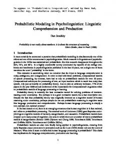
Figure 2. Schematic of the methodology used for the distribution of an aggregate’s volume into defined size fractions. Subroutines from Press et al. [1992] were used for the solution of the nonlinear differential system of equations for the aggregation operator. One subroutine is based on the Rosembrock method [Kaps and Rentrop, 1979; Press et al., 1992]; the other is based on the semi-implicit extrapolation method [Bader and Deuflhard, 1983; Press et al., 1992]. Both subroutines use lower-upper triangular (LU) decomposition for solving the linear systems generated. The user of these subroutines has to provide algorithms for the numerical evaluation of the system of the differential equations and their Jacobian. All the algorithms have been coded in C using the Microsoft Visual C/C⫹⫹ version 5.0 compiler. The operator-splitting approach allows the modeler the flexibility to select independently the subroutines to be used to solve the settling and aggregation terms. As stated in section 3, no analytical solution exists for the general Smoluchowski equation. However, for the very particular case in which the initial particle population is monodisperse (i.e., a single particle size) and where the collision frequency function is constant for all types of collisions, the analytical solution is [Smoluchowski, 1917]: n i⌬t ⫽

n 10共0.5 ␤ constantn 10⌬t兲 i⫺1 . 共1 ⫹ 0.5 ␤ constantn 10⌬t兲 i⫹1

(16)

This analytical solution provides a means to test the numerical schemes proposed, provided that the same constraints are applied to the numerical algorithm tested. Jacobson et al. [1994] have used this analytical expression to test their algorithms for solving the Smoluchowski equation. To test the validity of the solution for more general cases, the Rosembrock method and the semi-implicit method were compared against each other. For both the particular case of the analytical solution and for the selected more general cases the agreement was complete. To discretize the initial particle population and assign the aggregates formed to the fractions defined by our initial discretization, we followed the approach used by Lawler et al. [1980]. We divided the size population using equally spaced logarithmic diameter increments. The volume of the aggregates resulting from collisions between particles of the different size fractions results in volume sizes different from the ones of the defined fractions. To address this problem, a fraction of the aggregate was assigned to the size fraction imme-

diately smaller, and the rest were assigned to the size fraction immediately larger. The portion assigned to each size fraction is proportional to the ratio between the difference of the volumes of the new aggregate and the size fraction divided by the difference between the volumes of the two size fractions. Figure 2 (case a) depicts the methodology described. Because of the finite nature of the discretization of the particle population, aggregates larger than the largest size fraction (v m ⬎ v NS) are assigned to the largest size fraction. In order to preserve volume (mass), the volume of aggregates larger than v NS is divided by the volume of v NS. The resulting ratio (v m /v NS) is assumed to be the number of new particles of the largest size fraction produced by an aggregate larger than v NS (Figure 2, case b). Mass balances were used to test mass allocation between different size fractions and as a further check of the subroutines used to calculate the differential equations and their Jacobian.

6. Comparison of Proposed Scheme Versus Traditional Scheme for the Case of a Quiescent System To compare the solutions of the PTA equation for the case of a quiescent system using the upwind (a first-order discretization) and the residence-time scheme, two cases were modeled. In the first case we modeled a system with no aggregation (␣ ⫽ 0, pure settling); in the second case we modeled a system with maximum aggregation (␣ ⫽ 1). The column was discretized into equally spaced vertical compartments. The last compartment is considered the bottom of the column, where particles settle and accumulate, and is used for verifying mass balance; plots of modeling results do not include this compartment. The particle size range was discretized into diameter fractions uniformly spaced on a logarithmic scale. The initial loading of particles includes only the top five compartments; the rest are filled with fluid only. This choice allows a better visualization of the effect of numerical diffusion on settling of sharp fronts of suspended material, pulse inputs of different suspensions, or water bodies with inhomogeneous spatial particle size distributions. The initial number concentration of each particle size fraction was calculated using the following expression [Lawler et al., 1980; Valioulis and List, 1984]:

2254

PERIGAULT ET AL.: MODELING PARTICLE TRANSPORT AND AGGREGATION

Table 2. Properties and Parameters Used for Settling and Settling-Aggregation Simulations Parameter

Symbol ⌬z NC NS

Depth of each compartment Number of compartments Number of sizes Size range Power law exponent Concentration factor Mass concentration Particle’s density Fluid’s density Temperature Fluid’s viscosity Velocity gradient Time step

␤ A ␳suspension ␳solid ␳fluid T ␮ G ⌬t

⌬N ⫽ n共v兲⌬v,

⌬v m ⫽ ⫽

冉

vm ⫹

冊 冉

v m⫹1 ⫺ v m ⫺ 2

vm ⫺

v m ⫺ v m⫺1 2

冊

v m⫹1 ⫺ v m⫺1 . 2

(18)

In various natural systems, n(v) has been found to follow a power law behavior [Lerman, 1977; Lawler et al., 1980; O’Melia and Bowman, 1984; Pizarro et al., 1995; Jackson and Burd, 1998]: n共v兲 ⫽

2A 共d v兲 ⫺共2⫹␤兲, ␲

(19)

where A is a coefficient related to the total concentration of particulate matter and the exponent ␤ is found to lie in the range 2–5. A value ␤ ⫽ 4 has often been used to model particulate matter in lakes and settling tanks [Lerman, 1977; Lawler et al., 1980; O’Melia and Bowman, 1984; Pizarro et al., 1995; Jackson and Burd, 1998]. The physical significance of ␤ ⫽ 4 is that the volume of particulate material in suspension is evenly distributed among the logarithmically spaced size fractions; in other words, every logarithmically spaced size fraction contains the same amount of particulate volume. All the simulations in this paper used a power law distribution with ␤ ⫽ 4. Table 2 lists the values for the other parameters used for the simulations. Simulation results for number and volume concentrations are presented in the format traditionally used by researchers working with particle concentration distributions [Lawler et al., 1980; Hunt, 1982; O’Melia and Bowman, 1984; Valioulis and List, 1984]. Number concentrations are represented as the logarithm of the total suspended-particle number concentration in a logarithmic interval of particle diameter dv: log

再

dN d共log d v兲

冎

⫽ log 兵2.3Ad v共1⫺␤兲其.

(20)

Volume concentrations are represented as the total suspended-particle volume concentration in a logarithmic interval of particle diameter d v :

Units

8 50 30 1–30 4 5.4 ⫻ 10⫺6 17 2 1 25 8.91 ⫻ 10⫺4 0.05 15

cm dimensionless dimensionless ␮m dimensionless m3 m⫺3 mg L⫺1 g mL⫺1 g mL⫺1 ⬚C kg m⫺1 s⫺1 s⫺1 s

dV 2.3 ␲ ⫽ Ad v共4⫺␤兲. d共log d v兲 6

(17)

where ⌬N is the number concentration of particles with volume within a given volume range (⌬v represents a volume differential). For a given size fraction (n m ) the size distribution function is evaluated using the volume of the size fraction (v m ). The volume differential used is the difference between the upper limit and the lower limit of the volume range assigned to that fraction, which we have defined as

Value

7.

(21)

Discussion

Results for the case of pure settling (␣ ⫽ 0) are depicted in Figures 3a and 3b. Because of the use of a power law distribution the initial number concentration of larger particles is very small compared with the number concentrations of the smaller ones, therein is the reason to represent number concentrations as log {dN/[d(log d v )]}. The presentation of the results in this format allows a better visualization of the effect of numerical diffusion present in the upwind scheme. Both at times 100 and 240 min, the number concentration peaks and spatial concentration profiles differ from the ones at the initial time. The simulations show a spatial Gaussian spreading of the initial concentrations over time, resulting in number concentrations with a wider range and smaller maximums compared with the profiles at the initial time. Both behaviors should not occur under a pure settling regime and are numerical artifacts. However, the RTS preserves the profile of the initial concentrations. The results of pure settling using the RTS at times 100 and 240 min show the different fractions settling “as a pack,” which is consistent with the physical behavior expected. The differences between the upwind and RTS schemes are more obvious in the volume concentration results. Clearly, the numerical diffusion inherent to the upwind, first-order scheme produced a misallocation of an important fraction of the volume of the larger sizes and significantly lower concentrations at depths in which, according to Stokes’ settling regime, particles are. The results for the second case, settling and aggregation, are depicted in Figures 4a and 4b. In this case, differences are more dramatic. The main reason is the dependence of aggregation rates on the square of the concentrations (equations (1), (3), and (4)). As mentioned in section 3, the main effect of numerical diffusion is to spread the concentrations over the reactor volume, producing concentration misallocation and lower maximum concentrations. As a result, the upwind scheme decreases the aggregation rate in the areas of maximum concentration and increases aggregation in other zones. As expected, the major differences are observed for the volume concentrations. For natural systems, researchers have proposed a range for ␤ between 2 and 5 [Lawler et al., 1980; Hunt, 1982; O’Melia and Bowman, 1984; Valioulis and List, 1984; Pizarro et al., 1995].

PERIGAULT ET AL.: MODELING PARTICLE TRANSPORT AND AGGREGATION

2255

Figure 3a. Results of simulation of settling of a polydisperse suspension with no aggregation (␣ ⫽ 0) using the first-order finite difference scheme. The differences presented using ␤ ⫽ 4 will be more noticeable for values of ␤ ⬍ 4 and will be less noticeable for ␤ ⬎ 4. For values under ␤ ⫽ 4 the initial distribution will contain more large particles (which are subject to larger numerical diffusion); for values above 4 the opposite effect is expected. Simulations at higher concentrations were performed but not presented in this paper. They showed that when aggrega-

tion is considered, higher loadings produced larger differences between the simulations performed using the upwind scheme and the RTS. This is expected because higher concentrations increase aggregation rates, shifting particle populations toward larger sizes, which are more affected by numerical diffusion. The use of two different solvers for the aggregation term allowed the verification of the algorithm for cases for which

2256

PERIGAULT ET AL.: MODELING PARTICLE TRANSPORT AND AGGREGATION

Figure 3b. Results of simulation of settling of a polydisperse suspension with no aggregation (␣ ⫽ 0) using the residence-time scheme (RTS).

analytical solutions are not available. For the conditions used for the simulations presented, no differences regarding computational efficiency and accuracy were found between the results provided by the Rosembrock method and the semiimplicit method.

8.

Summary and Concluding Remarks

The residence-time scheme (RTS) allows the modeling of particle settling in a way that prevents the introduction of numerical diffusion or instabilities. Particle transport phenom-

PERIGAULT ET AL.: MODELING PARTICLE TRANSPORT AND AGGREGATION

2257

Figure 4a. Results of simulation of settling of a polydisperse suspension with aggregation (␣ ⫽ 1) using the first-order finite difference scheme. ena, such as particle settling and aggregation, can be effectively modeled using the alternating-operator-splitting technique (AOST). A polydisperse system of particles was modeled under pure settling (␣ ⫽ 0) and settling and aggregation (␣ ⫽ 1) regimes. Clearly, for both cases, there are significant differences be-

tween the results obtained using the traditional first-order discretization (upwind scheme) and the RTS. Notable are the large differences in volume distributions and volume concentrations of the different fractions observed. The differences observed between the results of the upwind first-order finite differences and RTS show that numerical diffusion can intro-

2258

PERIGAULT ET AL.: MODELING PARTICLE TRANSPORT AND AGGREGATION

Figure 4b. Results of simulation of settling of a polydisperse suspension with aggregation (␣ ⫽ 1) using the residence-time scheme (RTS) for settling. duce serious errors. The magnitude of this artifact is not equal for all the fractions but is a function of size, time increments, and compartment length. RTS is a robust and efficient alternative for modeling particle settling because of its mathematical simplicity, numerical efficiency, and lack of numerical artifacts. The flexibility of the

AOST methodology allows the modeler to include additional processes, such as turbulent transport, chemical processes, etc., without having to rewrite and validate the subroutines used for other processes. The independent solution of each term allows the use of the best numerical or analytical alternative for each process. Because the transport and aggregation of particles are

PERIGAULT ET AL.: MODELING PARTICLE TRANSPORT AND AGGREGATION

controlled by a number of physicochemical processes, modularity is a particularly useful feature.

Appendix: Schematic Description of the ResidenceTime Scheme (RTS) for Particle Settling A schematic description of the residence-time scheme (RTS), written as a pseudocode, is presented in Figure A1. This algorithm applies for settling of a polydisperse suspension of particles through a one-dimensional fluid column. There is no mass transfer between the first compartment and the top of the column. The last compartment is considered the bottom of the tank (nothing settles out of it). All column compartments are assumed to have the same length (⌬z). The first (initial) time step is set up equal to the residence time of the largest (fastest) size fraction. The time steps used for the solution of the aggregation operator are not necessarily equal to the time steps used for solving the settling operator.

2259

Notation C m Courant number for a particle of settling velocity W m [dimensionless]. d v spherical diameter of a particle of volume v [L]. D m numerical diffusion coefficient for a particle of volume m [L 2 T ⫺1 ]. g gravitational acceleration [L T ⫺2 ]. G fluid mean velocity gradient [T ⫺1 ]. k b Boltzman’s constant [ J K ⫺1 ]. n(v) size distribution function in terms of particle volume [number L ⫺6 ]. 0 n 1 number concentration of a monodisperse suspension of particles at time zero [number L ⫺3 ]. ⌬t number concentration of a particle formed ni by i particles from the original

Figure A1. Schematic description of the residence-time scheme (RTS).

2260

PERIGAULT ET AL.: MODELING PARTICLE TRANSPORT AND AGGREGATION

n m,k t n m,k

N NC

NS

T Qz v vm V Wv W max size ⌬N ⌬t ⌬z

monodisperse suspension n 01 after a time step ⌬t [number L ⫺3 ]. number concentration of particles in size fraction m in compartment k [number L⫺3]. number concentration of particles of size fraction m in compartment k at time t [number L ⫺3 ]. total number concentration of particles [number L ⫺3 ]. number of vertical subdivisions (compartments) in which the fluid column is discretized [number]. number of logarithmically spaced size fractions in which the particle population is discretized [number]. fluid temperature [degrees]. vertical fluid velocity [L T ⫺1 ]. particle volume [L 3 ]. particle volume of fraction m [L 3 ]. total volume concentration of particles [L 3 L ⫺3 ]. Stokes’ settling velocity for a particle of volume v [L T ⫺1 ]. Stokes’ settling velocity for largest particle [L T ⫺1 ]. number concentration of particles with volume within a given volume range [number L ⫺3 ]. time step [T]. depth of vertical discretization [L].

Greek letters A concentration coefficient of power law size distribution [L ␤ ⫺1 L ⫺3 ]. ␣ (v*, v ⫺ v*) collision efficiency between a particle of volume v* and a particle of volume v ⫺ v* [dimensionless]. ␤ exponent of power law size distribution [dimensionless]. ␤ constant constant collision frequency function [L3 T⫺1]. ␤ (v*, v ⫺ v*) Brownian collision frequency function due to Brownian motion between a particle of volume v* and a particle of volume v ⫺ v* [L 3 T ⫺1 ]. ␤ (v*, v ⫺ v*) settling collision frequency function due to differential settling between a particle of volume v* and a particle of volume v ⫺ v* [L 3 T ⫺1 ]. ␤ (v*, v ⫺ v*) shear collision frequency function due to fluid shear between a particle of volume v* and a particle of volume v ⫺ v* [L 3 T ⫺1 ]. ␤(v*, v ⫺ v*) total collision frequency function between a particle of volume v* and a particle of volume v ⫺ v* [L 3 T ⫺1 ]. ␤ i, j,k total collision frequency function between a particle of size fraction i and a particle of size fraction j in compartment k [L3 T⫺1]. ␧ z vertical mixing coefficient [T ⫺1 ]. ␳ fluid fluid’s density [M L ⫺3 ]. ␳ solid solid’s density [M L ⫺3 ].

␳ suspension concentration of suspended solid (mass concentration) [M L ⫺3 ]. ␮ fluid’s dynamic viscosity [M L ⫺1 T ⫺1 ]. ␶ m residence time for a particle of settling velocity W m in a compartment of depth ⌬z [T]. Acknowledgments. This work was funded by NSF grant CTS9422962, “Particle Aggregation and Sedimentation in a Continuous Flow, Gravity-Driven System.” The third author was supported by NSF grant EAR-9522651, “Factors Controlling Solute Dilution in Heterogeneous Aquifers.” The authors are grateful to Wendell P. Ela, University of Arizona at Tucson, and Alexander P. Robertson and Amresh Prasad, Stanford University, for their thoughtful comments and discussions. The authors would like to thank Stanley B. Grant, University of California, Irvine, and two anonymous reviewers for their suggestions and thorough revision of the manuscript.

References Ali, W., C. R. O’Melia, and J. K. Edzwald, Colloidal stability of particles in lakes: Measurement and significance, Water Sci. Technol., 17, 701–712, 1984. Bader, G., and P. Deuflhard, A semi-implicit mid-point rule for stiff systems of ordinary differential equations, Numer. Math., 41, 373– 398, 1983. Boehm, A. B., and S. B. Grant, Influence of coagulation, sedimentation, and grazing by zooplankton on phytoplankton aggregate distributions in aquatic systems, J. Geophys. Res., 103(C8), 15,601– 15,612, 1998. Davis, R. H., The rate of coagulation of a dilute polydisperse system of sedimenting spheres, J. Fluid Mech., 145, 179 –199, 1984. Friedlander, S. K., Smoke, Dust and Haze, John Wiley, New York, 1977. Gardner, K. H., Chemical effects on particle aggregation kinetics, Ph.D. thesis, Clarkson Univ., Potsdam, N. Y., 1995. Grant, S. B., C. Poor, and S. Relle, Scaling theory and solutions for the coagulation and settling of fractal aggregates in aquatic systems, Colloids Surf. A, 107, 155–174, 1996. Han, M. Y., and D. F. Lawler, Interactions of two settling spheres: Settling rates and collision efficiencies, J. Fluid Mech., 117, 145–179, 1991. Han, M. Y., and D. F. Lawler, The (relative) insignificance of G in flocculation, J. Am. Water Works Assoc., 84, 79 –91, 1992. Hunt, J. R., Particle dynamics in seawater: Implications for predicting the fate of discharged particles, Environ. Sci. Technol., 16, 303–309, 1982. Islam, M. R., and M. H. Chaudhry, Numerical solution of transport equation for applications in environmental hydraulics and hydrology, J. Hydrol., 191, 103–121, 1997. Jackson, G. A., and A. B. Burd, Aggregation in the marine environment, Environ. Sci. Technol., 32, 2805–2814, 1998. Jacobson, M. Z., R. P. Turco, E. J. Jensen, and O. B. Toon, Modeling coagulation among particles of different composition and size, Atmos. Environ., Part A, 28, 1327–1338, 1994. Jiang, Q., and B. E. Logan, Fractal dimensions of aggregates determined from steady-state size distributions, Environ. Sci. Technol., 25, 2031–2038, 1991. Johnson, C. P., and B. E. Logan, Settling velocities of fractal aggregates, Environ. Sci. Technol., 30, 1911–1918, 1996. Kaluarachchi, J. J., and J. Morshed, Critical assessment of the operator-splitting technique in solving the advection-dispersion-reaction equation, 1, First-order reaction, Adv. Water Resour., 18(2), 89 –100, 1995a. Kaluarachchi, J. J., and J. Morshed, Critical assessment of the operator-splitting technique in solving the advection-dispersion-reaction equation, 2, Monod kinetics and coupled transport, Adv. Water Resour., 18(2), 101–110, 1995b. Kaps, P., and P. Rentrop, Generalized Runge-Kutta methods of order four with stepsize control for stiff ordinary differential equations, Numer. Math., 33, 55– 68, 1979. Lawler, D. F., C. R. O’Melia, and J. E. Tobiason, Integral water treatment plant design: From particle size to plant performance, in Particulates in Water, edited by M. C. Kavanaugh and J. O. Leckie, Am. Chem. Soc., Washington, D. C., 1980.

PERIGAULT ET AL.: MODELING PARTICLE TRANSPORT AND AGGREGATION Lerman, A., Geochemical Processes: Water and Sediments Environments, John Wiley, New York, 1977. Li, X., and B. E. Logan, Collision frequencies of fractal aggregates with small particles by differential sedimentation, Environ. Sci. Technol., 31, 1229 –1236, 1997a. Li, X., and B. E. Logan, Collision frequencies between fractal aggregates and small particles in a turbulently sheared fluid, Environ. Sci. Technol., 31, 1237–1242, 1997b. Liang, L., Effects of surface chemistry on kinetics of coagulation of submicron iron oxide particles (␣-Fe2O3) in water, Ph.D. thesis, Calif. Inst. of Technol., Pasadena, 1988. McCarthy, J. F., and J. M. Zachara, Subsurface transport of contaminants, Environ. Sci. Technol., 23, 496 –502, 1989. McGauhey, P. H., Theory of sedimentation, J. Am. Water Works Assoc., 48, 437– 448, 1956. O’Melia, C., and K. S. Bowman, Origins and effects of coagulation in lakes, Schweiz. Z. Hydrol., 46(1), 64 – 85, 1984. Parker, D. S., W. J. Kaufman, and D. Jenkins, Floc breakup in turbulent flocculation processes, J. Sanit. Eng. Div. Am. Soc. Civ. Eng., 98(SA1), 79 –99, 1972. Pizarro, J., N. Belzile, M. Filella, G. G. Leppard, J. C. Negre, D. Perret, and J. Buffle, Coagulation/sedimentation of submicron iron particles in a eutrophic lake, Water Res., 29(2), 617– 632, 1995. Press, W. H., S. A. Teukolsky, W. T. Vetterling, and B. P. Flannery, Numerical Recipes in C, Cambridge Univ. Press, New York, 1992. Smoluchowski, M., Versuch einer Mathematischen Theorie der Koagulations Kinetic Kolloider Lo ¨sungen, Z. Phys. Chem., 92, 129 –168, 1917. Spielman, A. L., Viscous interactions in Brownian coagulation, J. Colloid Interface Sci., 33(4), 562–571, 1970.

2261

Tannehill, J. C., Hyperbolic and hyperbolic-parabolic systems, in Handbook of Numerical Heat Transfer, edited by W. J. Minkowycz et al., pp. 463– 476, John Wiley, New York, 1988. Tiller, C. L., and C. R. O’Melia, Natural organic matter and colloidal stability: Models and measurements, Colloids Surf. A, 73, 89 –102, 1993. Valioulis, I. A., and E. J. List, Numerical simulation of a sedimentation basin, 1, Model development, Environ. Sci. Technol., 18, 242–247, 1984. Valocchi, A. J., and M. Malmstead, Accuracy of operator splitting for advection-dispersion-reaction problems, Water Resour. Res., 28(5), 1471–1476, 1992. Verwey, E. J. W., and J. T. G. Overbeek, Theory of the Stability of Lyophobic Colloids, Elsevier Sci., New York, 1948. Warming, R. F., P. Kutler, and H. Lomax, Second- and third-order non-centered difference schemes for nonlinear hyperbolic equations, AIAA J., 11(2), 189 –196, 1973. Wilson, B. N., and B. J. Barfield, Modeling sediment detention ponds using reactor theory and advection-diffusion concepts, Water Resour. Res., 21(4), 523–532, 1985. P. K. Kitanidis, J. O. Leckie, and J. G. Perigault, Department of Civil and Environmental Engineering, Terman Engineering Center, Stanford University, Stanford, CA 94305-4020 (kitanidis@ce. stanford.edu; [email protected]; [email protected])

(Received August 13, 1999; revised March 30, 2000; accepted March 31, 2000.)

2262