is made by a probing phase and a shrinking phase. During the probing ... reduced to one if a retransmission timeout expires [10]. AIMD-based .... eâλRn fRn (R)dR = Râ(λ),. (3) ...... Fluid-based analysis of a network of AQM routers supporting ...
Modeling the AIADD Paradigm in Networks with Variable Delays G. Boggia, P. Camarda, A. D’Alconzo, ∗ L. A. Grieco, and S. Mascolo DEE - Politecnico di Bari - Via Orabona, 4 70125 BARI, Italy
E. Altman, C. Barakat INRIA 2004, route des lucioles 06902 Sophia Antipolis {eitan.altman, chadi.barakat}@sophia.inria.fr
{g.boggia, camarda, a.dalconzo, a.grieco, mascolo}@poliba.it
ABSTRACT Modeling TCP is fundamental for understanding Internet behavior. The reason is that TCP is responsible for carrying a huge quota of the Internet traffic. During last decade many analytical models have attempted to capture dynamics and steady-state behavior of standard TCP congestion control algorithms. In particular, models proposed in literature have been mainly focused on finding relationships among the throughput achieved by a TCP flow, the segment loss probability, and the round trip time (RTT) of the connection, which the flow goes through. Recently, Westwood+ TCP algorithm has been proposed to improve the performance of classic New Reno TCP, especially over paths characterized by high bandwidth-delay products. In this paper, we develop an analytic model for the throughput achieved by Westwood+ TCP congestion control algorithm when in the presence of paths with time-varying RTT. The proposed model has been validated by using the ns-2 simulator and Internet-like scenarios. Validation results have shown that this model provides relative prediction errors smaller than 10%. It has been shown that a similar accuracy is achieved by analogous models proposed for New Reno TCP. Moreover, it has been proved that it is necessary to consider delay variability in modeling Westwood+ TCP; otherwise, if only the average RTT is considered, performance could be underestimated.
Keywords TCP Congestion Control, TCP Modelling, Performance Evaluation
1. INTRODUCTION TCP congestion control was introduced by Van Jacobson in the cornerstone paper [16] with the main objectives to obtain ∗Corresponding author.
a high Internet utilization while avoiding network collapse due to congestion. Many improvements to the Jacobson’s congestion control algorithm, also known as Tahoe TCP, have been proposed during last decade by the Internet Engineering Task Force (IETF) [21, 2, 1, 12]. All the proposed TCP enhancements are based on the well-known Additive Increase Multiplicative Decrease (AIMD) paradigm, which is made by a probing phase and a shrinking phase. During the probing phase, a TCP sender additively increases its own congestion window, which limits the number of outstanding segments, to probe network for new available bandwidth until a network congestion is revealed by the reception of 3 Duplicated Acknowledgments (DUPACKs) or the expiration of a retransmission timeout. During the shrinking phase, and in order to recover the network from congestion, the congestion window is halved when 3 DUPACKs are received or reduced to one if a retransmission timeout expires [10]. AIMD-based algorithms, such as New Reno TCP [12], exhibit poor performance in the presence of random losses and paths with high bandwidth-delay product [18]. So that, more sophisticated paradigms for finely tuning TCP congestion window would be required [19]. Recently, to overcome AIMD performance limitations, Westwood TCP and its Westwood+ variant [20, 14] have been proposed. Both of them are based on the new Additive Increase ADaptive Decrease (AIADD) paradigm, which leaves unchanged the probing phase of New Reno TCP and proposes an adaptive shrinking phase. In particular, the adaptive decrease used by Westwood TCP sets the congestion window according to the bandwidth left behind TCP at time of congestion, which is the end-to-end network available bandwidth as defined in [14]. The available bandwidth is estimated by properly processing the stream of returning ACKs. Westwood+ variant differs from the original one in that it employs an enhanced bandwidth estimation scheme, which is robust with respect to ACK compression [23]. Modeling TCP is fundamental for understanding Internet behavior. The reason is that TCP carries a very large quota of Internet traffic [8]. As a consequence, during the last decade, many analytical models have attempted to capture dynamic and steady-state behavior of standard TCP congestion control algorithms [25, 17, 22, 5]. In particular, those studies have mainly focused on the relationships be-
tween TCP throughput, the segment loss probability, and the round trip time (RTT) seen by a TCP sender. In [25], a simple analytical characterization of the steadystate throughput of Reno TCP [11] as a function of the loss rate and RTT for a bulk data transfer has been developed. Three models are proposed: the first one assumes only 3 DUPACKs reception as congestion indication; the second one considers also timeouts; the third one is a simplification of the second one. The models have been validated against traces collected from the real Internet; results have shown that even using the most accurate model, i.e., the second one, prediction errors can be up to 100% in some circumnstances. In [17], an approach for dealing with issues concerning the stability and the fairness of IP networks has been proposed. A part of the analytical arguments proposed in [17] has been later exploited in [15] to develop steady-state models for the throughput of Westwood+ TCP congestion control algorithm. In [22], the attention has been focused on modeling the dynamics of TCP congestion control using a fluid approach. In particular, a stochastic dynamic model for TCP congestion window has been proposed in state-space domain. Then the proposed model has been used for designing Active Queue Management (AQM) algorithms. In [9], a similar approach has been followed for deriving a dynamic model for Westwood TCP. Approaches cited so far do not consider the impact of RTT variability on TCP throughput. Recently the importance of this issue has been discussed in [5], where a closed-form expression for the throughput of a TCP connection going through a path with a time-varying delay has been derived. Models proposed in [5] consider classical TCP implementations deriving from the Reno algorithm but more recent TCP congestion control algorithms such as Westwood+ TCP have not been yet investigated. In order to bridge this gap, this paper proposes an analytical model for the throughput of a Westwood+ TCP connection going through a path with variable delays using theoretical arguments from [5] and [15]. Our study aims at capturing the behavior of the Westwood+ algorithm under realistic hypothesis, i.e., time varying delays, which hold in almost all packet switching networks and that are usually not taken into account. One can encounter delay variability in wireless networks due to mobility and link-level retransmissions. It can also be observed in wired networks due to load balancing and changes in the routing tables. Our findings have been validated by exploiting the ns-2 simulator with Internet-like scenarios. Validation results have shown that model we propose provides relative prediction errors smaller than 10%. It has been shown that a similar accuracy is achieved by analogous models proposed for New Reno TCP in [5]. Moreover, it has been considered the effect of delay variability on Westwood+ TCP modeling. In particular, it has been proved that performance could be underestimated with an analytical model assuming a constant RTT.
2.
BACKGROUND ON RENO, NEW RENO, AND WESTWOOD+ TCP
A TCP connection is characterized by the following variables: (1) congestion window (cwnd); (2) slow start threshold (ssthresh); (3) round trip time of the connection (RT T ); (4): minimum round trip time measured by the sender (RT Tmin ). The pseudo-code of the Reno algorithm is reported below (see Algorithm 1). if ACKs are successfully received then if cwnd < sstresh then cwnd = cwnd + 1; else cwnd = cwnd + 1/cwnd; end else if 3 DUPACKs are received by the sender then ssthresh = cwnd/2; if ssthresh < 2 then ssthresh=2; cwnd = ssthresh; else if a coarse timeout expires then ssthresh = cwnd/2; if ssthresh < 2 then ssthresh = 2; cwnd=1; end Algorithm 1: Pseudo-code of Reno algorithm.
When 3 DUPACKs are received, the Reno TCP algorithm enters the fast recovery phase and retransmits the segment with the lowest unacknowledged sequence number. This phase is leaved when the retransmitted segment is successfully acknowledged. NewReno differs from Reno TCP in that it does not exit the fast recovery phase until all the segments within the current window are acknowledged. This feature, which is known as NewReno feature, improves the performance of Reno TCP when several segments within the same window get lost [12]. The key idea of TCP Westwood+ is to exploit the stream of returning acknowledgment packets to estimate the bandb that is available for the TCP connection. When a width B congestion episode happens at the end of the TCP probing phase, the bandwidth estimated from the stream of ACKs corresponds to the definition of best effort available bandwidth in a connectionless packet network. This bandwidth estimate is used to adaptively decrease the congestion window and the slow-start threshold after a timeout or three duplicate ACKs as it is described below (see Algorithm 2). It is worth noting that the adaptive decrease mechanism employed by Westwood+ TCP improves the standard TCP multiplicative decrease algorithm. In fact, the adaptive window shrinking provides a congestion window that is sufficiently decreased in the presence of heavy congestion and not excessively so in the presence of light congestion or losses that are not due to congestion, such as in the case of unreliable radio links. Moreover, the adaptive setting of the congestion window increases the fair allocation of available bandwidth to different TCP flows. In fact, if for sake of simplicity we neglect the normalization factor seg size, it could
Moreover, it is a good approximation when packets of a TCP connection are lost due to other factors that congestion induced by the connection itself, for example when the connection crosses many routers with exogenous traffic [4], or when it crosses wireless links with transmission errors.
if ACKs are successfully received then if cwnd < sstresh then cwnd = cwnd + 1; else cwnd = cwnd + 1/cwnd; end
Thus, probability that in a generic interval Rn there are no loss packets (i.e., Zn = 0) is equal to
else if 3 DUPACKs are received by the sender then b · RT T ssthresh = B min ; if ssthresh >
>
∗ : B 1
=
=
∗ + (1 − Z )β = (1 − Z0 )W0∗ + RT Tmin Z0 B 0 0
N X
+α
=
(27)
=
N X
E [(1 − Z0 )W0∗ 1{ζ(1) = j}] h
h
i
ci wi Pij + α
N X
�
+βE [(1 − Z0 )1{ζ(1) = j}] .
ci = E
(28)
�
1 1 − α ζ(0) = i ≈ (1 − α) . R0 E[R0,i ]
(34)
When all wj are computed, we have
E [(1 − Z0 )W0∗ 1{ζ(0) = i}1{ζ(1) = j}]
i=1
+RT Tmin
(33)
where E[R0,i ] is the mean value of Rn at state i and = 1/E[R0,i ] is the approximation of E[1/R0,i ], as in eq. (17).
Considering all the possible states at T0 ,
N X
bi Pij .
i=1
The parameters ci are given by.
i
∗ 1{ζ(1) = j} +RT Tmin E Z0 B 0
N X
�
∗ 1{ζ(0) = i} P = E B ij 0
i=1
wj
=
N X
1 − α ζ(0) = i E [W0∗ 1{ζ(0) = i}] Pij R0
i=1
Hence,
wj
�
E
i=1
.
W∗
∗ = (1 − α) 0 + αB 0 R0
∗ · 1{ζ(1) = j}] E[B 1 �� � � 1−α
∗ E W0∗ + αB 0 1{ζ(1) = j} R0
h
E[W0∗ ] =
i
∗ 1{ζ(0) = i}1{ζ(1) = j} E Z0 B 0
N X
wj .
(35)
j=1
i=1
+β
N X
3.4
E[(1 − Z0 )1{ζ(0) = i}1{ζ(1) = j}]
i=1
=
N X
E [(1 − Z0 )|ζ(0) = i] E [W0∗ 1{ζ(0) = i}] Pij
i=1
+RT Tmin
N X
h
E[Z0 |ζ(0) = i]E
∗ B
i 0 1{ζ(0)
N X i=1
E[(1 − Z0 )|ζ(0) = i]πi Pij .
X=
E[W0∗ ] . E[R0 ]
(36)
= i} Pij
i=1
+β
Throughput Analysis
The expression of E[W0∗ ] can be used for throughput evaluation. In fact, in general the throughput X of a long lived TCP connection is given by:
(29)
When Rn are correlated, eq. (36) has to be evaluated numerically using the derivation in sec. 3.3, whereas when Rn are i.i.d. it is possible to find a closed form for throughput.
In fact, from (19): X=
R∗ (λ) β · . E[R0 ] − RT Tmin 1 − R∗ (λ)
(37)
Such an expression can be rewritten as a function of probability pwr that there is at least one congestion window reduction due to a loss event. It is worthwhile to note that pwr is not the loss packet probability, given that in the same RTT time can be more packet losses, but only one window reduction. Let λ′ be the rate of window reduction. Obviously, λ′ ≤ λ, given that λ is the packet loss rate, and λ′
= =
mean number of events which reduce window E[R0 ] E[Z0 = 1] 1 − R∗ (λ) = . (38) E[R0 ] E[R0 ]
Rate λ′ is also given by product between probability of window reduction pwr and throughput: λ′ = pwr X.
(39)
Thus, from eqs. (38) and (39) R∗ (λ) = 1 − E[R0 ]pwr X.
(40)
in the interval [1 s, 7000 s]. Links connecting nodes hosting FTP cross-traffic sources and sinks have a delay of 25 ms. Other links have a delay of 2.5 ms. The link capacity between routers is equal to 2 Mbps. The capacity of entry/exit links is 1000 Mbps. TCP segments are 1500 Bytes long. The overhead due to lower layer protocols is neglected. Buffers are 42 packets long, which is the bandwidth-delay product that would be obtained with a 2 Mbps link with RTT=250 ms. The number of hops N has been varied from 2 to 20 and for each scenario 30 simulations have been executed, each one using a different seed for the ns-2 random number generator. For each repetition, we have evaluated the average value of the congestion window of the C1 connection over the time and we have compared the so obtained value with respect to the windows’ values predicted using eqs. (19) and (35) of the model, when the C1 connection employs Westwood+ as congestion control algorithm, and using analogous models reported in [5] when New Reno is used. To analyze the effect of delay variability on performance estimation of Westwood+ TCP, we have also reported the congestion windows obtained without taking into account correlation among RTT samples. To this aim, we have to consider all RTTs constant and equal to their average value E[R0 ] as in other models already present in literature (e.g., see [25]). Thus, eq. (3) becomes P (Zn = 0) = R∗ (λ) = e−λE[R0 ] .
(43)
Substituting the last equation in (19), we can find throughput X as a function of pwr . The term R∗ (λ), which takes into account RTT variability, disappears, but impact of delay variation figures in pwr .
and we obtain
For Rn i.i.d., using eq. (40) in (37):
In the following, when eq. (35) is used, we will consider a two state Markov model for describing Rn . In particular, for each of the 30 simulations, the set of collected Rn has been split into two subsets, one for each of the states of the Markov model. The first subset is made by Rn values smaller than a threshold value RT Tth , the second one contains the other Rn values. RT Tth has been varied by spanning all collected RTT values. For each selected threshold a different parameter set of the two-state Rn model has been obtained, to which corresponds a different prediction of the congestion window. Among all the obtained predictions, we will consider the one closer to the measured average congestion window. An analogous approach has been considered when we have used correlated Rn with the New Reno model proposed in [5].
1 − E[R0 ]pwr X β · X= . E[R0 ] − RT Tmin E[R0 ]pwr X
(41)
It can be easily checked that this equation has a real and positive solution: p
(pwr βE[R0 ])2 + 4βpwr E[R0 ]∆R , 2pwr E[R0 ]∆R (42) where ∆R = (E[R0 ] − RT Tmin ). X=
−pwr βE[R0 ] +
4. MODEL VALIDATION In this section theoretical models represented by eqs. (19) and (35) will be validated by using the ns-2 simulator with Internet-like scenarios. Moreover, analogous models proposed in [5] for New Reno TCP will been validated. We will consider the multihop topology depicted in Fig. 2, which is characterized by: (a) N hops; (b) one greedy TCP connection C1 (which we take either Westwood+ or New Reno) going through all the N hops; (c) N cross traffic New Reno TCP connections C2 ÷ CN +1 transmitting data over each single hop. The simulation lasts 10000 s during which the C1 connection always sends data. Each cross traffic source C2 ÷ CN +1 starts randomly in the interval [100 s, 3000s ], and lasts for a random time uniformly distributed
E[W0∗ ] =
βE[R0 ] e−λE[R0 ] · . E[R0 ] − RT Tmin 1 − e−λE[R0 ]
(44)
Fig. 3 reports for each value of N both measured and estimated average cwnd obtained when the C1 connection employs Westwood+ as congestion control algorithm. Also confidence intervals at 95% are reported for simulation results. In particular, Fig. 3.a reports the estimated average cwnd obtained assuming correlated Rn and using eq. (35), Fig. 3.b reports analogous data obtained considering i.i.d. Rn and using eq. (19), and, similarly, Fig. 3.c shows the same data obtained using eq. (44). By comparing Figs. 3.a, 3.b, and 3.c, it is straightforward to note that model using correlated Rn is the most accurate.
Sink3
C3
Sink5
C5
SinkN+1
smaller than 7 (resp. 4), errors are smaller than 8% (4%) and exhibit statistical fluctuations that depend on the interactions between C1 and the other C2 ÷ CN +1 connections, which are difficult to predict (see also [6]).
CN+1
C1
Sink1
C2
Sink2
C4
Sink4
Ci – ith connection
CN
SinkN
Sinki – ith sink
Figure 2: Multibottleneck topology. Moreover, assuming i.i.d. Rn leads to a small prediction improvement with respect to the case of a assuming a constant RT T . Thus, in order to avoid performance underestimation, it is necessary to take into account correlation among RTTs also when Westwood+ TCP is adopted. Note that in this scenario a lower throughput is achieved with Westwood+. In fact, the competing New Reno cross traffic, after congestion, does not deplete router buffers as Westwood+; thus, the C1 connection with Westwood+ grabs an amount of bandwidth smaller than when it uses New Reno. However, this result does not affect model accuracy. The same conclusions can be derived by looking at Fig. 4 where analogous data obtained for New Reno TCP have been reported. In order to better quantify modeling improvements obtained assuming correlated Rn rather than i.i.d. Rn , Fig. 5 reports the relative errors obtained for Westoowd+ and New Reno. It is straightforward to note that assuming correlated Rn leads to relative errors one order of magnitude smaller than the ones in the cases where i.i.d. Rn or constant RTT are assumed. By looking with more attention at Fig. 5, new insights into model behaviors can be found. In fact, when correlated Rn are assumed, in the case of Westwood+ (resp. New Reno) it can be noticed that relative errors start increasing monotonically when the number of hops traversed by the C1 connections is larger than 7 (resp. 4). The reason is that when the number of hops increases it is more likely that cwnd dynamics are driven by timeouts expiration rather than 3 DUPACKs receptions. Thus, relative errors increases with the number of hops because slow start and cwnd backoff have not been modeled. This can be confirmed by looking at Fig. 6 reporting the cwnd of the C1 connection averaged over the 30 simulations. In particular, Fig. 6 clearly highlights that, when a scenario with 10 hops is considered, both New Reno and Westwood+ keep the cwnd at 1 for a very large quota of the simulation time. On the other hand, when a scenario with 4 hops is simulated, the measured average cwnd is larger than 1 for almost all the simulation time. On the other hand, when the number of traversed hops is
Thus it can be concluded that the proposed model is able to capture the behavior of Westwood+ TCP with a relative prediction error smaller than 10%. Moreover both the model we have proposed and the analogous one proposed for New Reno in [5] provide similar accuracies.
5.
CONCLUSION
In this paper, an analytical model for the throughput of Westwood+ TCP in networks with variable delays has been developed. The model has been built starting from recent theoretical findings reported in literature [5] [15]. The proposed model, which does not take into account timeout events, has been validated by means of ns-2 simulations of Internet-like scenarios. Results have shown that analytical framework herein describes is able to capture Westwood+ TCP behavior with relative prediction errors smaller than 10%. Moreover, it has been shown that the same accuracy is provided by analogous models proposed in literature for New Reno TCP. The main finding of this paper is that a great modeling accuracy can be achieved by considering the correlation among RTT samples; otherwise, there could be significant errors in TCP performance estimation by exploiting analytical models.
22.5 22.5 Analitically estimated average cwnd Measured average cwnd
17.5 cwnd [TCP Segments]
Measured average cwnd
17.5 cwnd [TCP Segments]
20.0
Analitically estimated average cwnd
20.0
15.0 12.5 10.0 7.5
15.0 12.5 10.0 7.5 5.0
5.0
2.5 2.5
0.0 0.0
0 0
1
2
3
4
5
6
7
8
9
10
1
2
3
11
4
Number of hops - N -
7
8
9
10
11
22.5
22.5
Analitically estimated average cwnd
20.0
20.0
Measured average cwnd
Analitically estimated average cwnd
17.5 cwnd [TCP Segments]
17.5 cwnd [TCP Segments]
6
(a)
(a)
Measured average cwnd
15.0 12.5 10.0 7.5
15.0 12.5 10.0 7.5
5.0
5.0
2.5
2.5 0.0
0.0 0
1
2
3
4
5 6 7 Number of hops - N -
8
9
10
0
11
1
2
3
4
5
6
7
8
9
10
11
Number of hops - N -
(b)
(b)
22.5
22.5
20.0
Analitically estimated average cwnd
20.0
Measured average cwnd
17.5
Analitically estimated average cwnd Measured average cwnd
cwnd [TCP Segments]
17.5 cwnd [TCP Segments]
5
Number of hops - N -
15.0 12.5 10.0 7.5 5.0
15.0 12.5 10.0 7.5 5.0
2.5
2.5
0.0 0
1
2
3
4
5 6 7 Number of hops - N -
8
9
10
11
(c) Figure 3: Analytically Estimated and Measured Average cwnd of Westwood+: (a) Correlated Rn ; (b) i.i.d. Rn ; (c) mean RTT.
0.0 0
1
2
3
4
5
6
7
8
9
10
11
Number of hops - N -
(c) Figure 4: Analytically Estimated and Measured Average cwnd of New Reno: (a) Correlated Rn ; (b) i.i.d. Rn ; (c) mean RTT.
100
70 4 Hops Average cwnd [TCP Segments]
Relative error [%]
60
10
1 Correlated R n i.i.d. R n Mean RTT
10 Hops
50 40 30 20 10 0
0.1 0
1
2
3
4
5
6
7
8
9
10
0
11
1000
2000
3000
4000
5000
6000
7000
8000
10000
(a)
(a) 70
100
4 Hops 10 Hops
Average cwnd [TCP Segments]
60
Relative error [%]
9000
Time [s]
Number of hops - N -
10
1 Correlated R n i.i.d. R n Mean RTT
50 40 30 20 10
0.1
0
0
1
2
3
4
5
6
7
8
9
10
11
Number of hops - N -
0
1000
2000
3000
4000
5000
6000
7000
8000
9000
10000
Time [s]
(b)
(b)
Figure 5: Model errors: (a) Westwood+; (b) New Reno.
Figure 6: Average cwnd: (a) Westwood+; (b) New Reno.
6. REFERENCES [1] M. Allman, S. Floyd, and C. Partridge. Increasing initial TCP’s initial window. RFC 3390, October 2002. [2] M. Allman, V. Paxson, and W. R. Stevens. TCP congestion control. IETF RFC 2581, April 1999. [3] E. Altman. Stochastic recursive equations with applications to queues with dependent vacations. Annals of Operations Research, 112:43–61, 2002. [4] E. Altman, K. Avratchenkov, and C. Barakat. A stochastic model of TCP/IP with stationary random losses. In Proc. of ACM Sigcomm 2000, Stockholm, Sweden, 2000. [5] E. Altman, C. Barakat, and V. M. R. Ramos. Analysis of AIMD protocols over paths with variable delay. Computer Networks, 48(6):960–971, Aug. 2005. [6] F. Baccelli and D. Hong. Interaction of TCP flows as billiards. In Proc. of IEEE Infocom’03, 2003. [7] A. Brandt. The stochastic equation Yn+1 = An Yn + Bn with stationary coefficients. Advances in Applied Probability, 18:211–220, 1986. [8] CAIDA. Cooperative association for internet data analysis. available at http://www.caida.org/, 2005. [9] J. Chen, F. Paganini, R. Wang, M. Y. Sanadidi, and M. Gerla. Fluid-flow Analysis of TCP Westwood with RED. In Proceedings of IEEE Globecom 2003, San Francisco, CA, November 2003. [10] D. Chiu and R. Jain. Analysis of the increase and decrease algorithms for congestion avoidance in computer networks. Computer Networks and ISDN Systems, 17(1):1–14, June 1989. [11] K. Fall and S. Floyd. Simulation-based Comparisons of Tahoe, Reno, and SACK TCP. Computer Communication Review, 26(3), July 1996. [12] S. Floyd, T. Henderson, and A. Gurtov. NewReno modification to TCP’s fast recovery. IETF RFC 3782, April 2004. [13] P. Glasserman and D. D. Yao. Stochastic vector difference equations with stationary coefficients. Journal of Applied Probability, 32:851–866, 1995. [14] L. A. Grieco and S. Mascolo. Performance evaluation and comparison of Westwood+, New Reno and Vegas TCP congestion control. ACM Computer Communication Review, 34(2):25–38, April 2004. [15] L. A. Grieco and S. Mascolo. Mathematical Analysis of Westwood+ TCP Congestion Control. IEE Proceedings Control Theory and Applications, 152(1):35–42, January 2005. [16] V. Jacobson. Congestion avoidance and control. In ACM Sigcomm ’88, pages 314–329, Stanford, CA, USA, August 1988. [17] F. Kelly. Mathematical modeling of the internet. In Fourth International Congress on Industrial and Applied Mathematics, Edinburgh, July 1999.
[18] T. V. Lakshman and U. Madhow. The Performance of TCP/IP for Networks with High Bandwidth-Delay Products and Random Loss. IEEE Transactions on Networking, 5(3):336–350, June 1997. [19] S. H. Low, F. Paganini, and J. C. Doyle. Internet congestion control. IEEE Control Systems Magazine, 22(1):28–43, February 2002. [20] S. Mascolo, C. Casetti, M. Gerla, M. Sanadidi, and R. Wang. TCP Westwood: End-to-end bandwidth estimation for efficient transport over wired and wireless networks. In ACM Mobicom 2001, Rome, Italy, July 2001. [21] M. Mathis, J. Mahdavi, S. Floyd, and A. Romanow. TCP Selective Acknowledgment Options. IETF RFC 2018, October 1996. [22] V. Misra, W.-B. Gong, and D. F. Towsley. Fluid-based analysis of a network of AQM routers supporting TCP flows with an application to RED. In SIGCOMM, pages 151–160, 2000. [23] J. C. Mogul. Observing TCP dynamics in real networks. In ACM Sigcomm ’92, pages 305–317, Baltimore, MD, USA, August 1992. [24] R. Nelson. Probability, Stochastic Processes, and Queueing Theory. Springer-Verlag, 1995. [25] J. Padhye, V. Firoiu, D. Towsley, and J. Kurose. Modeling TCP throughput: A simple model and its empirical validation. In ACM Sigcomm ’98, pages 303–314, Vancouver BC, Canada, 1998.
APPENDIX A. CHECKING OF CONDITION FOR STOCHASTIC EQUATION Herein, we will check conditions reported in [13] to establish that the stochastic vector recursive equation (9) admits a unique solution given by eq. (10) as n grows to infinity. The conditions to be verified are [13]: −∞ ≤
E[log A0 ]
E[log C 0 ]
< 0;
< ∞,
(45)
where k·k is a matrix (vector) norm. Note that index 0 refers to initial condition for An and C n , not to the steady state. It is well known that a matrix norm [13] has to verify the following properties: (i)
S
≥ 0 and
(ii) ∀a ∈ (iii) (iv)
S
S
R,
+T ·T
aS
S
≤
≤
= 0 if and only if S = 0;
≤ |a| S ;
S
S
·
+
T ;
T ;
while a vector norm has to verify only properties (i), (ii) e (iii). It can be easily checked that the following function is a norm:
S
= max{Sij } . i,j
(46)
Now, using norm (46), we can show that conditions (45) are verified. For what concerns vector C 0 defined in eq. (9) we have:
C 0
= |(1 − Z0 )β| = (1 − Z0 )β
(47)
and, evaluating its mean value:
E[ C 0 ] = E[(1 − Z0 )β] = R∗ (λ)β .
(48)
Now, by Jensen inequality [24] the following result holds:
E(log C 0 ) ≤ log E[ C 0 ] < ∞
(49)
that is, the second condition in (45). b in eq. For what concerns matrix A0 , note that Wn and B n (9) are dimensional variables. An appropriate selection of units of measurement can allow us to verify the first condition in (45).
In particular, if Wn is expressed in TCP segments and each Rn is expressed as multiple of the minimum value RT Tmin , we have: RT Tmin = 1.
(50)
Moreover, s s Rn ≥ RT Tmin ∀n ⇒ Rn ≥1 � � 1 1 ⇒ s ≤1 ⇒E ≤ 1, s Rn Rn s where Rn represents the Rn value scaled by RT Tmin .
(51)
Now, by definition Zn ≤ 1 and E[Zn ] = 1 − R∗ (λ) < 1, so that each term of matrix An in eq. (9) with n = 0 (i.e., the initial condition) is less or equal than 1. Therefore, considering the expectation of each term, we have: E [1 − Z0 ] < 1;
E[RT Tmin Z0 ] < 1; � 1−α E < 1; α < 1 ; R0s �
(52)
that is
E[ A0 ] < 1
(53)
Fianlly, applying Jensen inequality [24], also the first condition in (45) is verified:
−∞ ≤ E[log A0 ] ≤ log E[ A0 ] < 0 .
(54)