Modeling the Effect of Composition and Temperature on the ... - MDPI

minerals Article

Modeling the Effect of Composition and Temperature on the Conductivity of Synthetic Copper Electrorefining Electrolyte Taina Kalliomäki *, Jari Aromaa and Mari Lundström Department of Materials Science and Engineering, School of Chemical Technology, Aalto University, P.O. Box 16200, Aalto FI-00076, Finland; [email protected] (J.A.); [email protected] (M.L.) * Correspondence: [email protected]; Tel.: +358-40-734-8658 Academic Editor: William Skinner Received: 1 March 2016; Accepted: 13 June 2016; Published: 24 June 2016

Abstract: The physico-chemical properties of the copper electrolyte significantly affect the energy consumption of the electrorefining process and the quality of the cathode product. Favorable conditions for electrorefining processes are typically achieved by keeping both the electrolyte conductivity and diffusion coefficient of Cu(II) high, while ensuring low electrolyte viscosity. In this work the conductivity of the copper electrorefining electrolyte was investigated as a function of temperature (50–70 ˝ C) and concentrations of copper (Cu(II), 40–60 g/L), nickel (Ni(II), 0–20 g/L), arsenic (As(III), 0–30 g/L) and sulfuric acid (160–220 g/L). In total 165 different combinations of these factors were studied. The results were treated using factorial analysis, and as a result, four electrolyte conductivity models were built up. Models were constructed both with and without arsenic as the presence of As(III) appeared to cause non-linearity in some factor effects and thus impacted the conductivity in more complex ways than previously detailed in literature. In all models the combined effect of factors was shown to be minor when compared to the effect of single factors. Conductivity was shown to increase when copper, nickel and arsenic concentrations were decreased and increase with increased temperature and acidity. Moreover, the arsenic concentration was shown to decrease the level of conductivity more than previously suggested in the literature. Keywords: copper electrorefining electrolyte; conductivity; conductivity model

1. Introduction Copper electrorefining is the most common method for producing high-purity copper [1]. The first refinery (Pembrey Copper Works) was established in 1869 following the first patent for commercial electrorefining developed by James Elkington in 1865 [2,3]. Since then, the process has been developed further as the result of both research and improved industrial practices [2]. In the copper electrorefining process, copper is dissolved from impure copper anodes into the electrolyte bath and then subsequently deposited on to cathodes as high-purity copper [4]. Industrial copper refining electrolytes mainly consist of water, copper sulfate, sulfuric acid, with additional leveling/grain-refining agents—to obtain smoother and denser cathode deposits—and process impurities [4,5]. These impurities commonly consist of nickel, arsenic and iron, along with smaller amounts of bismuth, antimony and chloride that dissolve into the electrolyte from the anode. The physico-chemical properties of the copper electrolyte significantly affect the yield of cathodic copper in the electrorefining process and include four main physico-chemical properties: conductivity, density, viscosity and the diffusion coefficient of the cupric ion (Cu(II)) [5–11]. The best yield of copper can be obtained by keeping the electrolyte viscosity low [5] while ensuring a high diffusion coefficient [7] and electrical conductivity [5]. These properties of the copper electrolyte are strongly

Minerals 2016, 6, 59; doi:10.3390/min6030059

www.mdpi.com/journal/minerals

Minerals 2016, 6, 59

2 of 11

influenced by composition and temperature: Increased temperature, for example, lowers electrolyte density and viscosity [6] while enhancing the rate of chemical reactions [4]. On the other hand, a too-high temperature results in unnecessary energy costs and excessive electrolyte bath evaporation [4]. In contrast, an electrolyte composition with a high concentration of Cu(II), Ni(II) and sulfuric acid makes the electrolyte denser and more viscous [6,12]. An increase in viscosity decreases the diffusion coefficient of Cu(II) but a high concentration of Cu(II) also increases the limiting current density [7], giving the possibility for a higher deposition rate. Moreover, an increase in the concentration of sulfuric acid leads to enhanced conductivity [5–7]. As a result, it is important to thoroughly determine the effects of these parameters in order to optimize the yield of cathode copper. Conductivity is an important solution property [13] as it affects the electrical energy consumption of the electrorefining process [5,6]. Therefore, when optimizing the refining process by altering the temperature or composition, conductivity is a good value to be controlled either by measuring it or defining it with an applicable model. The aim of this study is to construct accurate mathematical models for the conductivity, taking into account the effect of temperature as well as solution sulfuric acid and metal concentrations. Furthermore, a particular focus is also paid to the effect of typical impurities such as nickel and arsenic, originating from increasingly impure raw materials in addition to copper. The design of experiments is carried out with full factorial design by MODDE software (MKS Data Analytics Solutions, Malmö, Sweden) in order to build up a model that reflects copper electrorefining conductivity as a function of all the previously mentioned parameters. 2. Materials and Methods Electrolytes were prepared from copper sulfate (CuSO4 ¨ 5H2 O, min. 98%, VWR Chemicals, Radnor, PA, USA), nickel sulfate (NiSO4 ¨ 6H2 O, min. 98%, VWR Chemicals), sulfuric acid (H2 SO4 , 95%–98%, Sigma-Aldrich, St. Louis, MO, USA), arsenic acid solution (from Boliden Harjavalta Copper electrorefinery, Harjavalta, Finland, containing [As] = 151,700 mg/L, [Cu] = 4794 mg/L, [Sb] = 3954 mg/L, [Ni] = 1688 mg/L, [Bi] = 6.2 mg/L, [Te] = 18.6 mg/L, [Pb] = 29 mg/L, [Ag] = 0.16 mg/L) and distilled water. Cu and Ni contents in arsenic acid were also taken into account when preparing the electrolytes. Table 1 summarizes the experimental factors and solution parameters studied, 33 different solution parameter combinations were investigated at five different temperatures and in total 165 different combinations were studied. No extra additives such as glue, thiourea or chloride ions were used. Table 1. Parameters investigated affecting copper electrorefining electrolyte—factors ([Cu(II)], [H2 SO4 ], [Ni(II)], [As(III)] and temperature, T) and their levels. Arsenic was adjusted by arsenic acid (Cu(II) and Ni(II) in acid taken into account). Factor Cu(II) H2 SO4 Ni(II) As(III) T

Levels 40; 50; 60 160; 180; 200; 220 0; 10; 20 0; 15; 30 50; 55; 60; 65; 70

g/L g/L g/L g/L ˝C

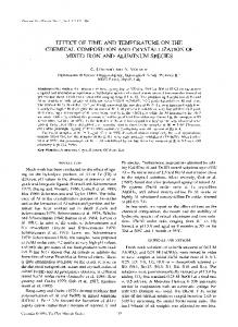
Conductivity measurements were carried out using a Knick Portamess® 913 Cond conductivity meter produced by Knick Elektronische Messgeräte GmbH & Co. KG (Berlin, Germany). The meter was used with a four-electrode sensor (ZU 6985) which has glass/platinum measuring system and glass casing tube. All electrolytes were heated prior to measurement in a jacketed cell using a MGW Lauda MT/M3 circulating water bath (Figure 1) (LAUDA, Lauda-Königshofen, Germany). During the heating or between the measurements, the cell was completely covered and all the holes in the

Minerals 2016, 6, 59 Minerals 2016, 6, 59

3 of 11 3 of 10

(DOE) and multivariate data evaporation analysis. Theand experiments werewater designed defining factors, lid were plugged to prevent consequently loss.by The electrolyte wasresponses stirred at and levels of the factors using the full factorial design. 400 rpm using a magnetic stirrer.

Figure 1. of the set-up used used for for conductivity measurements: (a) (a) water water bath; bath; Figure 1. Schematic Schematic of the experimental experimental set-up conductivity measurements: (b) (b) magnetic magnetic stirrer; stirrer; (c) (c) jacketed jacketed cell; cell; and and (d) (d) conductivity conductivity sensor. sensor.

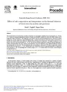
Prior modeling, raw data design was explored and evaluated with plots and histograms. Data to analysis and the experiment were carried out using thescatter Modeling design tool The models were constructed to the data and evaluated using regression analysis(DOE) tools MODDE 8 software (MKS Data according Analytics Solutions, Malmö, Sweden) for design of experiments summary of fit, analysis of variance (ANOVA) and normal probability plot of residuals. In addition, and multivariate data analysis. The experiments were designed by defining factors, responses and the designs checked to ensure a low design. enough condition number, i.e., the ratio of the minimum levels of the were factors using the full factorial and maximum singular values of the factors. For a good design thiswith value is lessplots thanand 3, whereas in a Prior to modeling, the raw data was explored and evaluated scatter histograms. bad design is over 6 [14]. The according effect of the the models after refining was also determined The modelsitwere constructed tochanges the datainand evaluated using regression analysis tools by comparison the change in value(ANOVA) of the condition number. summary of fit,of analysis of variance and normal probability plot of residuals. In addition, In summary, the parameters the model are goodness of fit goodnessand of the designs were checked to ensure athat low describe enough condition number, i.e., the ratio of (R the2),minimum 2 prediction (Q ), model validity reproducibility. Model this validity on the lack of fitinwhich maximum singular values of theand factors. For a good design valueisisbased less than 3, whereas a bad is a statistical F-test where model error is compared to replicate [14].was In aalso valid model there design it is over 6 [14]. Thethe effect of the changes in the models after error refining determined by is no lack of fit, and consequently the model validity is high. The reproducibility describes the comparison of the change in value of the condition number. variabilities in the replicates [14]. The models werethe refined to are maximize theseofcorrelation coefficients In summary, the parameters that describe model goodness fit (R2 ), goodness of 2 and Q2 values [14]. In a good model the Q2, the 2 as well as minimize the difference between the R prediction (Q ), model validity and reproducibility. Model validity is based on the lack of fit which is a model validity thethe reproducibility are larger than 0.5, 0.25 and respectively [14]. Inthere addition, statistical F-testand where model error is compared to replicate error0.5, [14]. In a valid model is no 2 and Q2 in a good model is less than 0.2–0.3 [14]. the the Rthe lackdifference of fit, and between consequently model validity is high. The reproducibility describes the variabilities in the replicates [14]. The models were refined to maximize these correlation coefficients as well as 3. Resultsthe anddifference Discussion minimize between the R2 and Q2 values [14]. In a good model the Q2 , the model validity and the aremeasured larger than 0.5, 0.25 anddata 0.5, is respectively [14]. In2 addition, Thereproducibility histogram of the conductivity shown in Figure and it canthe bedifference seen that 2 and Q2 in a good model is less than 0.2–0.3 [14]. between the R the histogram of the conductivity data is slightly skewed. The model validity and efficiency of data

Count

analysis are better when the data in the histogram plot is less skewed. Scatter plots of the raw data 3. Results and Discussion (Figure 3) showed both linearity and non-linearity which suggests that the relationship between some The histogram of themight measured conductivity is shown in Figure 2 andmay it can seen that factors and the response be curved, as welldata as the possibility that there be be interactions the histogram of theNevertheless, conductivity data slightly skewed. Thean model validity and efficiency of data between the factors. theseisscatter plots only give approximate estimation of how the analysiscan areinfluence better when the data in the histogram plot is less skewed. Scatter plots of the raw data factors the conductivity. (Figure 3) showed both linearity and non-linearity which suggests that the relationship between some factors and the response25might be curved, as well as the possibility that there may be interactions between the factors. Nevertheless, these scatter plots only give an approximate estimation of how the 20 factors can influence the conductivity. 15 10 5 0 435 465 495 525 555 585 615 645 675 705 735 765 795 825 mS/cm

Figure 2. Histogram of conductivity values of synthetic copper electrorefining electrolytes (for Model 1).

the histogram of the conductivity data is slightly skewed. The model validity and efficiency of data analysis are better when the data in the histogram plot is less skewed. Scatter plots of the raw data (Figure 3) showed both linearity and non-linearity which suggests that the relationship between some factors and the response might be curved, as well as the possibility that there may be interactions between the6,factors. Nevertheless, these scatter plots only give an approximate estimation of how Minerals 2016, 59 4 ofthe 11 factors can influence the conductivity. 25 Count

20 15 10 5 0 435 465 495 525 555 585 615 645 675 705 735 765 795 825 mS/cm

Figure 2.6,Histogram Histogram ofconductivity conductivityvalues valuesof ofsynthetic syntheticcopper copperelectrorefining electrorefiningelectrolytes electrolytes(for (forModel Model1).1).4 of 10 Minerals 2016,2. 59 Figure of

(a)

(b)

(c)

Figure 3. 3. Scatter Scatter plots plots of of the the raw raw data data for for synthetic synthetic copper copper electrolyte electrolyte with with factors factors (a) T and and Ni(II) Ni(II) Figure (a) T 2SO4 and As(III) concentration; and (c) H2SO4 and Cu(II) concentration. concentration; (b) H concentration; (b) H2 SO4 and As(III) concentration; and (c) H2 SO4 and Cu(II) concentration.

3.1. Conductivity Conductivity Model Model 1—Untreated 1—Untreated Data Data with with Terms Termsofof[H [H2SO SO4]]22 and T22 3.1. 2 4 and T In order order to to build build up up the the first first model model that that describes describes copper copper electrolyte electrolyte conductivity, conductivity, unscaled unscaled In conductivitydata datawas wasused. used. The model constructed thedata rawdespite data despite the skewed slightly conductivity The model waswas constructed from from the raw the slightly skewed nature of the data (Figure 2). nature of the data (Figure 2). Coefficients for for unrefined unrefined synthetic synthetic copper copper electrolyte electrolyte conductivity conductivity (Model (Model 1) 1) are are shown shown in in Coefficients Figure 4. 4. It be seen seen that that in in addition addition to to the the factors factors studied, studied, the the combined combined effect effect of of two two factors factors Figure It can can be (product) is also investigated. Terms with a high p-value (probability value), in which the error bars (product) is also investigated. Terms with a high p-value (probability value), in which the error bars extend over the zero line, need to be excluded from further analysis, e.g., the terms Cu(II)·H 2SO4 and extend over the zero line, need to be excluded from further analysis, e.g., the terms Cu(II)¨ H2 SO4 and Cu(II)·T for Model 1. The summary of fit for Model 1 showed that the R2, Q2 and reproducibility were at a good level, but the model validity was found to be poor. Model validity was improved by adding the squares of the terms to the model. Using squares [H2SO4]2 and T2, the irregularities of the normal probability plot could be reduced, although this was seen not to improve the model validity. Two result series (with a maximum amount of H2SO4, Cu(II) and Ni(II) as well as a maximum and medium amount of As(III)) were removed from the model, as it was suspected that these electrolytes were supersaturated and thus responsible for the skewness in


5 of 11

Cu(II)¨ T for Model 1. The summary of fit for Model 1 showed that the R2 , Q2 and reproducibility were at a good level, Minerals 2016, 6, 59 but the model validity was found to be poor. 5 of 10

Figure 4. Coefficients for unrefined synthetic copper electrolyte conductivity in Model 1. Adj. = Figure 4. Coefficients for unrefined synthetic copper electrolyte conductivity in Model 1. adjusted, Conf. lev. = confidence DF = degrees freedom, RSD =ofresidual standard Adj. = adjusted, Conf. lev. = level, confidence level, ofDF = degrees freedom, RSD deviation. = residual standard deviation. Table 2. R2, Q2, model validity and reproducibility values of the models. Model by adding 1 the squares 2 3 terms to 4 the model. Using squares Model validity was improved of the 2 2 2 R 0.9978 0.9985 0.9972 0.9984 [H2 SO4 ] and T , the irregularities of the normal probability plot could be reduced, although this was 2 0.9876 0.9959 (with 0.9661 0.9739 amount of H SO , Cu(II) seen not to improve the model Q validity. Two result series a maximum 2 4 Model validity 0.3016 0.4598 0.2609 0.4194 and Ni(II) as well as a maximum and medium amount of As(III)) were removed from the model, as it Reproducibility 0.9997 0.9996 0.9996 0.9996 was suspected that these electrolytes were supersaturated and thus responsible for the skewness in the results. Equation (1) for conductivity Model 1 was compiled according to unscaled coefficients. These modifications resulted in a reasonable model validity as well as slightly higher R2 and Q2 ; κ = 97.72number − 3.581 increased [Cu(II)] + from 0.47362.427 [Ni(II)] + 0.596 [As(III)] +data) 2.945to[H 2SO4] + however, the condition (with the unrefined 4.517—slightly high 2 2 0.02396 [Cu(II)][Ni(II)] + 0.006713 0.01219 [Ni(II)][As(III)] − fit in this but below 6—as a result of adding the terms [H[Cu(II)][As(III)] model had no lack of 2 SO4 ] and T . +The (1) 0.02297 [H2SO4][Ni(II)] − 0.02166 [Hthe 2SOmodel 4][As(III)] − 0.01899 + 0.01768 T[As(III)] phase and the summary of fit indicated that is valid (Table[Ni(II)]T 2). + 0.02754 [H2SO4]T + 2.743 T − 0.005364 [H2SO4]2 − 0.02946 T2 Table 2. R2 , Q2 , model validity and reproducibility values of the models.

where the concentrations are in g/dm3, T is in °C and κ is in mS/cm. The equation has many terms, and1 all the effects Model 2 of the factors 3 are not fully4seen in the equation coefficients. Nonetheless, factors with low p-values indicate that at least H2SO4 seems to have a 0.9978 0.9985 0.9972 0.9984 R2 combined effect with QNi(II), temperature and As(III). Data used for 1 indicated that Cu(II), 2 0.9876 0.9959 0.9661 Model 0.9739 Ni(II) and As(III)Model lowervalidity the conductivity while temperature0.4194 and H2SO4 increase it, 0.3016of the electrolyte 0.4598 0.2609 Reproducibility 0.9997 0.9996 0.9996 0.9996 which is in line with the literature [5,6]. 3.2. Conductivity 2—Logarithmic Data with compiled Terms of [H 2SO4]2 and T2 Equation (1)Model for conductivity Model 1 was according to unscaled coefficients. In order to avoid the skewness in Model 1 with untreated data, the second model was κ using “ 97.72 ´ 3.581 rCupIIqs rNipIIqsand ` 0.596 rAspIIIqsinà more 2.945 rH 2 SO4 s `distributed constructed logarithmic values` of 0.4736 conductivity this resulted normally histogram.0.02396 TermsrCupIIqsrNipIIqs with a high p-value were removed along with the two result series of the ` 0.006713 rCupIIqsrAspIIIqs ` 0.01219 rNipIIqsrAspIIIqs ´ (1) presumably supersaturated electrolytes determined from Model 1. As before, the term squares T2 and 0.02297 rH SO4 srNipIIqs ´ 0.02166 rH2 SO4 srAspIIIqs 0.01899 rNipIIqsT ` 0.01768 TrAspIIIqs ` [H2SO 4]2 were 2added to reduce the irregularities of the ´ normal probability plot. 2 using unscaled 2 Equation (2) for0.02754 the logarithm of the conductivity was rH compiled coefficients. The rH2 SO4 sT ` 2.743 T ´ 0.005364 2 SO4 s ´ 0.02946 T strongest combined effects based on low p-values were shown to be with H2SO4·T, H2SO4·As(III) and 3 , T is in ˝ C and κ is in mS/cm. where thehowever, concentrations are in g/dm T·As(III); as with Model 1, the combined effects were minor compared to the single effects The equation has many terms, and all the effects of the factors are not fully seen in the equation of factors. coefficients. Nonetheless, factors with low p-values indicate that at least H2 SO4 seems to have a log10(κ) = 2.17388 − 0.0023479 [Cu(II)] − 0.0027733 [Ni(II)] − 0.00073729 [As(III)] + 0.0037764 [H2SO4] − 1.0649 × 10−5 [H2SO4][As(III)] + 2.1627 × 10−5 T[As(III)] + (2) 8.8019 × 10−6 [H2SO4]T + 0.0051846 T − 6.9222 × 10−6 [H2SO4]2 − 3.2506 × 10−5 T2, Model 2 was regarded as reasonable and better with respect to Model 1, due to the improved model validity and Q2 value, and Q2 was almost equal to R2 (Table 2). However, the condition number


6 of 11

combined effect with Ni(II), temperature and As(III). Data used for Model 1 indicated that Cu(II), Ni(II) and As(III) lower the conductivity of the electrolyte while temperature and H2 SO4 increase it, which is in line with the literature [5,6]. 3.2. Conductivity Model 2—Logarithmic Data with Terms of [H2 SO4 ]2 and T2 In order to avoid the skewness in Model 1 with untreated data, the second model was constructed using logarithmic values of conductivity and this resulted in a more normally distributed histogram. Terms with a high p-value were removed along with the two result series of the presumably supersaturated electrolytes determined from Model 1. As before, the term squares T2 and [H2 SO4 ]2 were added to reduce the irregularities of the normal probability plot. Equation (2) for the logarithm of the conductivity was compiled using unscaled coefficients. The strongest combined effects based on low p-values were shown to be with H2 SO4 ¨T, H2 SO4 Äs(III) and TÄs(III); however, as with Model 1, the combined effects were minor compared to the single effects of factors. log10 pκq “ 2.17388 ´ 0.0023479 rCupIIqs ´ 0.0027733 rNipIIqs ´ 0.00073729 rAspIIIqs ` 0.0037764 rH2 SO4 s ´ 1.0649 ˆ 10-5 rH2 SO4 srAspIIIqs ` 2.1627 ˆ 10-5 TrAspIIIqs `

(2)

8.8019 ˆ 10-6 rH2 SO4 sT ` 0.0051846 T ´ 6.9222 ˆ 10-6 rH2 SO4 s2 ´ 3.2506 ˆ 10-5 T2 , Minerals 2016, 6, Model 2 59 was

6 of 10 regarded as reasonable and better with respect to Model 1, due to the improved 2 2 2 model validity and Q value, and Q was almost equal to R (Table 2). However, the condition number 4.456 was was over over3,3,asaswas wasthe thecondition condition number Model 1, but 6, which would indicate a 4.456 number of of Model 1, but not not overover 6, which would indicate a poor poor model. The condition number of this model was, however, lower than in Model 1. model. The condition number of this model was, however, lower than in Model 1.

3.3. Conductivity Data without without Arsenic Arsenic 3.3. Conductivity Model Model 3—Untreated 3—Untreated Data The third third conductivity conductivity model modelwas wasconstructed constructedwithout withoutthe theexperiments experimentscontaining containing arsenic and The arsenic and it it was found out thatthe thedata datawas wasquite quitenormally normallydistributed distributed(Figure (Figure5). 5).Scatter Scatter plots plots without without arsenic arsenic was found out that did not plots with according to to these these did not vary vary remarkably remarkably from from the the corresponding corresponding plots with arsenic. arsenic. Analogously, Analogously, according plots, Cu(II) and Ni(II) were shown to lower the conductivity while temperature and H 2 SO 4 were plots, Cu(II) and Ni(II) were shown to lower the conductivity while temperature and H2 SO4 were shown to to increase it. This seems to to have have slightly slightly better shown increase it. This model, model, however, however, seems better linearity linearity in in the the relationships relationships between the factors and the response than that observed in Models 1 and 2 which include the effect effect between the factors and the response than that observed in Models 1 and 2 which include the of As(III). Thus, As(III) seems to cause non-linearity in the model and also affects the conductivity in of As(III). Thus, As(III) seems to cause non-linearity in the model and also affects the conductivity in more complex complex ways ways than than would would be be expected expected from from the the literature literature [5,6,10]. [5,6,10]. more

Count

15 10 5 0 453 488 523 558 593 628 663 698 733 768 803 838 mS/cm

Figure 5. copper electrorefining electrolytes without the 5. Histogram Histogram of ofconductivity conductivityvalues valuesofofsynthetic synthetic copper electrorefining electrolytes without effect of arsenic (for (for Model 3). 3). the effect of arsenic Model

Model 33was wasrefined refined Model and compiled according to unscaled coefficients. The Model likelike Model 1 and1 compiled according to unscaled coefficients. The combined combined effect of H 2SO4·Ni(II) and H2SO4·T was shown to affect the conductivity value; however, effect of H2 SO4 ¨ Ni(II) and H2 SO4 ¨ T was shown to affect the conductivity value; however, the single the single parameters H2SOand 4, Ni(II) and T) had the biggest impact on conductivity. The sign parameters (Cu(II), H2(Cu(II), SO4 , Ni(II) T) had the biggest impact on conductivity. The sign (˘) of (±) of an individual variable or combined effect of variables equationshould shouldnot notbe be interpreted interpreted an individual variable or combined effect of variables in in thethe equation individually, but as a combined effect of all variables that have an effect in the equation. Figure 6 shows the effect of Ni(II) and T on the conductivity according to Equation (3), which indicates increased conductivity with increased temperature and decreased nickel concentration. Model validity was good according to the summary of fit (Table 2).

Figure 5. Histogram of conductivity values of synthetic copper electrorefining electrolytes without the effect of arsenic (for Model 3).

Model 3 was refined like Model 1 and compiled according to unscaled coefficients. The combined Minerals 2016,effect 6, 59 of H2SO4·Ni(II) and H2SO4·T was shown to affect the conductivity value; however, 7 of 11 the single parameters (Cu(II), H2SO4, Ni(II) and T) had the biggest impact on conductivity. The sign (±) of an individual variable or combined effect of variables in the equation should not be interpreted individually, but effect of all thatthat havehave an effect in thein equation. FigureFigure 6 shows individually, butasasa acombined combined effect of variables all variables an effect the equation. 6 the effect of Ni(II) and T on the conductivity according to Equation (3), which indicates increased shows the effect of Ni(II) and T on the conductivity according to Equation (3), which indicates conductivity with increased temperature decreased and nickeldecreased concentration. Model validity wasModel good increased conductivity with increased and temperature nickel concentration. according to the summary of fit (Table 2). validity was good according to the summary of fit (Table 2). κ “ 307.9 ´ 1.583 rCupIIqs ` 2.737 rNipIIqs ` 1.285 rH2 SO4 s ´ 0.02776 rH2 SO4 srNipIIqs ´ κ = 307.9 − 1.583 [Cu(II)] + 2.737 [Ni(II)] + 1.285 [H2SO4] − 0.02776 [H2SO4][Ni(II)] − 0.008774 rCupIIqsrH rNipIIqsT 2 SO 4s ´ 0.008774 [Cu(II)][H 2SO 4] 0.02087 − 0.02087 [Ni(II)]T`+0.02919 0.02919rH [H22SO SO44sT ]T ´ − 1.17 1.17 TT

(3) (3)

Figure 6. The Theeffect effectofoftemperature temperature and Ni(II) concentration on copper electrorefining electrolyte Figure 6. and Ni(II) concentration on copper electrorefining electrolyte using using Model 3, with [Cu(II)] = 50.51 g/L and [H 2SO4] = 182.842 g/L. Model 3, with [Cu(II)] = 50.51 g/L and [H SO ] = 182.842 g/L. 2

4

3.4. Conductivity Model 4—Without Arsenic and with Terms of [H2 SO4 ]2 and T2 The fourth conductivity model was constructed without arsenic data and by adding extra terms of [H2 SO4 ]2 and T2 , identical to Models 1 and 2. κ “ 31.863 ´ 1.3594 rCupIIqs ` 1.835 rNipIIqs ` 2.9789 rH2 SO4 s ´ 0.022681 rH2 SO4 srNipIIqs ´ 0.010403 rCupIIqsrH2 SO4 s ´ 0.021408 rNipIIqsT ` 0.02975 rH2 SO4 sT ` 2.7297 T ´ 2

(4)

2

0.0044364 rH2 SO4 s ´ 0.032787 T

Both Models 3 and 4 were shown to be valid according to the summary of fit (Table 2), with model validity being better than that of Model 3. Conversely, the condition number, 1.375, was better in Model 3 when compared to the value of 4.322 in Model 4. In contrast, the condition number of the unrefined design was 1.838. 3.5. Summary of the Models The defined Equations (1)–(4) are relatively complex due to the interactions of the factors, and thus the effects of the factors are impossible to directly see in the equations. The effects of Cu(II) and H2 SO4 on electrolyte conductivity containing the median amount of As(III) and Ni(II) at medium temperature, defined with Model 1, are presented in Figure 7a. Analogously, the effects of As and temperature containing a high amount of Cu(II), a low amount of H2 SO4 and a medium amount of Ni(II) are displayed in Figure 7b. Figure 8 presents the measured and predicted electrolyte conductivity values. It can be seen that the models predict the data with high correlation, with R2 varying from 0.9972 to 0.9985. In addition, the R2 , Q2 , model validity and reproducibility values of the models are presented in Table 2.

The defined Equations (1)–(4) are relatively complex due to the interactions of the factors, and thus the effects of the factors are impossible to directly see in the equations. The effects of Cu(II) and H2SO4 on electrolyte conductivity containing the median amount of As(III) and Ni(II) at medium temperature, defined with Model 1, are presented in Figure 7a. Analogously, the effects of As and temperature a high amount of Cu(II), a low amount of H2SO4 and a medium amount Minerals 2016, 6, containing 59 8 of of 11 Ni(II) are displayed in Figure 7b.


(a)

(b)

8 of 10

temperature to be similar according to [12] and this These comparisons are presented Figure 7. 7.seemed The Cu(II) and and H2SO 4 concentrations (a)work. as well as As(III) concentration and Figure The effect effect of of Cu(II) H 2 SO4 concentrations (a) as well as As(III) concentration and in Figure 9, where the equation by Devochkin et al. has been corrected due to an error in the sign of temperature (b) (b) on on copper copper electrorefining electrorefining electrolyte electrolyte (Model (Model 1), 1),with withTT==60 60˝°C, [Ni(II)]== 10.102 10.102g/L g/L temperature C, [Ni(II)] the Cu(II) concentration, was noticed testing equation their parameters 2SO4] = the 162.519 g/L andwith [Ni(II)] = 10.102 g/L (b). and and [As(III)] [As(III)] 15 g/L g/L (a) (a)which and [Cu(II)] [Cu(II)] 60.6125when g/L, [H [H and == 15 and == 60.6125 g/L, 2 SO4 ] = 162.519 g/L and [Ni(II)] = 10.102 g/L (b). comparing the results to their measured values. Figure 8 presents the measured and predicted electrolyte conductivity values. It can be seen that the models predict the data with high correlation, with R2 varying from 0.9972 to 0.9985. In addition, the R2, Q2, model validity and reproducibility values of the models are presented in Table 2. The effects of temperature, Cu(II), As(III) and Ni(II) on conductivity are presented in Figures 9–11. In addition to conductivity data calculated by Models 1–4, these figures present the corresponding literature values and in Figure 10 five measured values are also shown. The equation defined by Subbaiah and Das [8] was, however, not used in these comparisons, since it did not reproduce the values they presented in their paper even when their own parameters were used. This is probably due to the fact that their equation did not contain a Cu term, which possibly caused the discrepancy as that error was at minimum at low Cu(II) concentrations. Conductivity results obtained in this work were shown to be in good agreement with the previous research work of Price and Davenport [6]. Nevertheless, arsenic was shown to affect the conductivity slightly more and temperature less than determined by previous works [6,10]. Comparison of the results from this work to the equivalent results of Price and Davenport [6], Kern and Chang [10] and Devochkin et al. [12] shows that there were some differences between them. The Figure8. 8.Observed Observed(x) (x)versus versuspredicted predicted(y) (y)copper copper electrolyte conductivity values using Models 1–4. Figure conductivity values using Models 1–4. conductivity values were seen to be lower in [12] electrolyte than in the other studies. Conversely, the effect of

Conductivity (mS/cm)

160 g/l H2on SO4conductivity are presented in Figures 9–11. The effects of temperature, Cu(II), As(III) and Ni(II) 650 Model 2 (A) (B) In addition to conductivity data calculated by Models 1–4, these figures present the corresponding Price and Davenport (A) (B) literature values and in Figure 600 10 five measured values are also The equation defined by Devochkin et al., corrected equation (A) shown. (B) Subbaiah and Das [8] was, however, not used in these comparisons, since it did not reproduce the 550 values they presented in their paper even when their own parameters were used. This is probably due to the fact that their equation did500 not contain a Cu term, which possibly caused the discrepancy as that error was at minimum at low Cu(II) concentrations. 450 Conductivity results obtained in this work were shown to be in good agreement with the previous research work of Price and Davenport [6]. Nevertheless, arsenic was shown to affect the conductivity 400 slightly more and temperature less than determined by previous works [6,10]. Comparison of the 350 results from this work to the equivalent55results of [6], Kern and Chang [10] and 60 Price and 65 Davenport 70 Devochkin et al. [12] shows that there were some differences between them. The conductivity values T (°C) were seen to be lower in [12] than in the other studies. Conversely, the effect of temperature seemed to Figure 9. Effects of Cu(II), Ni(II) and temperature according to Model 2 from this work compared to be similar according to [12] and this work. These comparisons are presented in Figure 9, where the results of Price and Davenport [6] and Devochkin et al. [12]. (A) 50 g/L Cu(II), 18 g/L Ni(II) and equation by Devochkin et al. has been corrected due to an error in the sign of the Cu(II) concentration, (B) 65 g/L Cu(II), 24 g/L Ni(II). which was noticed when testing the equation with their parameters and comparing the results to their measured values. 65 °C, 160 g/l H SO , 40 g/l Cu(II) 2

700

vity (mS/cm)

680 660 640 620 600

4

0 g/l Ni(II), this work, measured 0 g/l Ni(II), Model 2 10 g/l Ni(II), Model 2 20 g/l Ni(II), this work, measured 20 g/l Ni(II), Model 2 20 g/l Ni(II), Price and Davenport


9 of 11

Figure 8. 8. Observed Observed (x) (x) versus versus predicted predicted (y) (y) copper copper electrolyte electrolyte conductivity conductivity values values using using Models Models 1–4. 1–4. Figure 160 g/l g/l H H2SO SO4 160 2 4

Conductivity Conductivity(mS/cm) (mS/cm)

650 650

Model 22 (A) (A) (B) Model (B) Price and and Davenport Davenport (A) (A) (B) Price (B) Devochkin et al., corrected equation (A) (A) Devochkin et al., corrected equation

600 600

(B) (B)

550 550 500 500 450 450 400 400 350 350

55 55

60 60

65 65

70 70

T (°C) (°C) T

Figure 9. 9. Effects of Cu(II), Ni(II) and temperature according toto Model from this work compared to Figure to Model 22 from this work compared to 9. Effects Effectsof ofCu(II), Cu(II),Ni(II) Ni(II)and andtemperature temperatureaccording according Model 2 from this work compared results of of Price and Davenport [6] and Devochkin etetal. al. [12]. (A) 50 g/L Cu(II), Cu(II), 18 g/L Ni(II) Ni(II) and results of Price and Davenport g/L to results Price and Davenport[6] [6]and andDevochkin Devochkinet al.[12]. [12]. (A) (A) 50 50 g/L g/L Cu(II), 18 18 g/L Ni(II) and (B) 65 65 g/L g/L Cu(II), 24 g/L Ni(II). (B) Cu(II), 24 g/L Ni(II). g/L Cu(II), 24 g/L Ni(II). 65 °C, °C, 160 160 g/l g/l H H2SO SO4,, 40 40 g/l g/l Cu(II) Cu(II) 65 2 4

Conductivity Conductivity(mS/cm) (mS/cm)

700 700 680 680

g/l Ni(II), Ni(II), this this work, work, measured measured 00 g/l g/l Ni(II), Ni(II), Model Model 22 00 g/l 10 g/l g/l Ni(II), Ni(II), Model Model 22 10 20 g/l g/l Ni(II), Ni(II), this this work, work, measured measured 20 20 g/l g/l Ni(II), Ni(II), Model Model 22 20 20 g/l Ni(II), Price and Davenport 20 g/l Ni(II), Price and Davenport

660 660 640 640 620 620 600 600 580 580 560 560 540 540 520 520 500 500

00

55

10 10

15 15

20 20

25 25

30 30

35 35

40 40

As(III) (g/l) (g/l) As(III)

Figure 10. 10. Effects Effects of Ni(II) and As(III) according to measured values and Model from this work work Figure Effects of of Ni(II) Ni(II) and and As(III) As(III) according according to to measured measured values values and and Model Model 222 from from this compared to results results of of Price Price and and Davenport Davenport [6]. [6]. Minerals 2016, 6, 59 9 of 10 compared to

Conductivity (mS/cm)

600

65 °C, 160 g/l H2SO4, 40 g/l Cu(II), 10 g/l Ni(II) Model 1 Model 2 Model 3 Model 4 Price and Davenport

590 580 570 560 550 0

5

10

15

20

25

30

As(III) (g/l)

11.Effects Effectsof of As(III) on copper electrorefining electrolyte conductivity using Figure 11. As(III) on copper electrorefining electrolyte conductivity defineddefined using Models Models this work and compared of Price and Davenport [6]. 1–4 from1–4 thisfrom work and compared to valuestoofvalues Price and Davenport [6].

Table 3 presents a comparison of values calculated with Models 1–4 and the model of Price and Davenport [6], Devochkin et al. [12] and measurements of Kern and Chang [10]. The model of Devochkin et al. was designed to determine conductivity from electrolytes without As(III) and with a constant Cu(II)/Ni(II) ratio; therefore, for that reason, their model was not used with all parameter combinations. The conductivity value determined using their model was lower than the other equivalent values, as can be observed in Figure 7. The values predicted by Models 1–4 were in good


10 of 11

Table 3 presents a comparison of values calculated with Models 1–4 and the model of Price and Davenport [6], Devochkin et al. [12] and measurements of Kern and Chang [10]. The model of Devochkin et al. was designed to determine conductivity from electrolytes without As(III) and with a constant Cu(II)/Ni(II) ratio; therefore, for that reason, their model was not used with all parameter combinations. The conductivity value determined using their model was lower than the other equivalent values, as can be observed in Figure 7. The values predicted by Models 1–4 were in good agreement with the values measured (Figure 8). Table 3. Comparison of values defined with Models 1–4 to equivalent values from Price and Davenport [6], Devochkin et al. [12] and to measured values from Kern and Chang [10]. κ (mS/cm)

Concentration (g/L) T (˝ C)

Model H2 SO4 Cu(II) Ni(II)

55 55 55 55 55

135 135 135 135 150

35 35 35 35 50

0 30 0 0 18

As(III) 0 0 30 40 0

1

2

3

4

538.4 453.4 504.8 493.6 478.0

534.0 440.9 498.9 487.7 475.0

536.9 472.1 485.8

528.3 456.1 479.9

Price and Davenport

Kern and Chang

527.3 458.4 516.7 513.2 477.8

530.7 444.0 523.1 519.4 -

Devochkin et al. 446.13

Furthermore, it can be seen that the values defined using the models detailed in this work also show a good correlation with both Kern and Chang’s results [10] and Price and Davenport (who reported a good agreement the results of Kern and Chang) [6]. According to this research, arsenic decreases conductivity and an improved model can be constructed. 4. Conclusions In this work the conductivity of the copper electrorefining electrolyte was investigated as a function of temperature (50–70 ˝ C) and concentrations of copper (Cu(II), 40–60 g/L), nickel (Ni(II), 0–20 g/L), arsenic (As(III), 0–30 g/L) and sulfuric acid (160–220 g/L). In total, 165 different combinations of these factors were studied. The measured data showed that conductivity was increased by a decrease in Cu(II), Ni(II) and As(III) concentration and increased with increasing temperature and acidity. As(III) appeared to affect the conductivity in more complicated ways than would be expected based on findings from the literature. In addition, it was observed that the untreated measured data was shown to be slightly skewed. The results were treated using factorial analysis, and as a result four different electrolyte conductivity models were created. Conductivity was measured reliably, and thus the models from the conductivity results were constructed directly. Combined effects were also detected, but the effects were minor compared to the effects of single factors. Model 1 was constructed from untreated conductivity data with terms of [H2 SO4 ]2 and T2 . Model 2 was constructed from logarithmic values of conductivity, also with additional terms of [H2 SO4 ]2 and T2 . Models 3 and 4 were constructed from untreated data by neglecting the measurement series with arsenic, and Model 4 with additional terms of [H2 SO4 ]2 and T2 . The four models constructed were all valid and had high correlation coefficients. In addition, the reproducibility was good, and the models did not suffer from a lack of fit. The most accurate models based on the best R2 , Q2 and model validity were Model 2 and Model 4 (Figure 8 and Table 2). Overall, this work provides improved models for copper electrolyte conductivity both in the presence and absence of arsenic. In particular, As(III) is shown to cause slight non-linearity and decrease conductivity more than previously reported, whereas temperature is shown to affect the electrolyte conductivity slightly less.


11 of 11

Acknowledgments: This research has been performed within the SIMP (System Integrated Metal Production) project of FIMECC (Finnish Metals and Engineering Competence Cluster Ltd. (Tampere, Finland)). Author Contributions: Taina Kalliomäki performed the experiments and analyzed the data as part of her Master’s thesis; Jari Aromaa counseled in experimental and theoretical matters as an instructor of the thesis; Mari Lundström and Taina Kalliomäki wrote the paper. All authors have read and approved the manuscript. Conflicts of Interest: The authors declare no conflict of interest.

References 1. 2.

3. 4. 5.

6. 7. 8. 9. 10. 11.

12.

13. 14.

Davenport, W.G.; King, M.; Schlesinger, M.; Biswas, A.K. Overview. In Extractive Metallurgy of Copper, 4th ed.; Elsevier Science Ltd.: Amsterdam, The Netherlands, 2002. Wraith, A.E.; Mackey, P.J.; Jones, R.P. Origins of electrorefining: Birth of the technology and the world’s first commercial electrofinery. In Proceedings of Copper 2013; The Chilean Institute of Mining Engineers: Santiago, Chile, 2013. Moats, M.S.; Hiskey, J.B. How anodes passivate in copper electrorefining. In The Copper 2010-Proceedings; GDMB: Hamburg, Germany, 2010; Volume 4. Davenport, W.G.; King, M.; Schlesinger, M.; Biswas, A.K.; Robinson, T. Electrolytic Refining. In Extractive Metallurgy of Copper, 4th ed.; Elsevier Science Ltd.: Amsterdam, The Netherlands, 2002; pp. 265–288. Price, D.C.; Davenport, W.G. Densities, electrical conductivities and viscosities of CuSO4 /H2 SO4 solutions in the range of modern electrorefining and electrowinning electrolytes. Metall. Trans. B 1980, 11, 159–163. [CrossRef] Price, D.C.; Davenport, W.G. Physico-chemical properties of copper electrorefining and electrowinning electrolytes. Metall. Trans. B 1981, 12, 639–643. [CrossRef] Moats, M.S.; Hiskey, J.B.; Collins, D.W. The effect of copper, acid, and temperature on the diffusion coefficient of cupric ions in simulated electrorefining electrolytes. Hydrometallurgy 2000, 56, 255–268. [CrossRef] Subbaiah, T.; Das, S.C. Physico-chemical properties of copper electrolytes. Metall. Trans. B 1989, 20, 375–380. [CrossRef] Jarjoura, G.; Muinonen, M.; Kipouros, G.J. Physicochemical properties of nickel copper sulfate solutions. Can. Metall. Q. 2003, 42, 281–288. [CrossRef] Kern, E.F.; Chang, M.Y. Conductivity of copper refining electrolytes. In Proceedings of the 41st General Meeting of the American Electrochemical Society, Baltimore, MD, USA, 28 April 1922. Skowronski, S.; Reinoso, E.A. The specific resistivity of copper refining electrolytes and method of calculation. In Proceedings of the 51st General Meeting of the American Electrochemical Society, Philadelphia, PA, USA, 30 April 1927. Devochkin, A.I.; Kuzmina, I.S.; Salimzhanova, E.V.; Petukhova, L.I. The study of sulfate copper electrolyte physicochemical properties depending on its components and temperature. Tsvetnye Met. 2015, 2015, 67–71. [CrossRef] Zhang, X.; Hu, Y.; Peng, X.; Yue, W. Conductivities of several ternary electrolyte solutions and their binary subsystems at 293.15, 298.15, and 303.15 K. J. Solut. Chem. 2009, 38, 1295–1306. [CrossRef] Eriksson, L.; Johansson, E.; Kettaneh-Wold, N.; Wikström, C.; Wold, S. Design of Experiments: Principles and Applications; MKS Umetrics AB: Malmö, Sweden, 2008. © 2016 by the authors; licensee MDPI, Basel, Switzerland. This article is an open access article distributed under the terms and conditions of the Creative Commons Attribution (CC-BY) license (http://creativecommons.org/licenses/by/4.0/).