of promoters in controlling the 'burstiness' of protein synthesis. Keywords: gene .... average rates of mRNA synthesis and protein generation. III. ... molecules attached to the gene-coding region of the DNA for a ..... state to move ribosome. L.
1
Modeling the stochastic dynamics of gene expression in single cells: A Birth and Death Markov Chain Analysis Samik Ghosh, Preetam Ghosh, Kalyan Basu and Sajal K. Das Biological Networking Research Group, Department of Computer Science & Engineering The University of Texas at Arlington, Arlington, TX 76010, USA. {sghosh, ghosh, basu, das}@cse.uta.edu
Aaj kaal er
Abstract— Fluctuations in protein number (noise) caused by the stochasticity in gene expression plays a central role in the dynamic behavior of cellular pathways. Deterministic models capture average cell population behavior and are limited in their relevance in modeling stochastic deviations of gene expression in single cells. In this paper, we develop a birth and death Markov chain model to capture the discrete molecular events of transcription and translation in prokaryotic cells. We derive mathematical models for the expression ‘burst frequency’ distribution as well as the number of protein molecules per burst. We validate our stochastic models with recent single cell experiments on the lacZ gene in Escherichia Coli and characterize expression noise sensitivity to biological parameters like gene activation ratio. Further, we build a discrete-event stochastic simulation system to study the transient dynamics of lacZ gene expression, quantifying the role of promoters in controlling the ‘burstiness’ of protein synthesis.
Keywords: gene expression, stochastic models, Markov chains, discrete event simulation
I.
INTRODUCTION
One of the key goals in studying complex cellular pathways is the understanding of the dynamic interaction between the cell’s gene regulatory and metabolic networks. In particular, the dynamics of protein-coding genes play a vital role in controlling the expression patterns of other genes encoding regulatory proteins and metabolic enzymes. Continuous and deterministic differential equation-based models representing the discrete molecular events of transcription and translation have been traditionally used to study gene expression in cell populations [1]. However, the inherent stochasticity in molecular interactions limits the applicability of these models in studying single cell expression deviations and observed cell-to-cell variability [1], [3], [4]. Stochastic fluctuations in the expression pattern of genes have been mathematically studied by
Arkin et. al [2], [5]and experimentally observed in [7], [8]. In particular, the ‘burstiness’ in protein production i.e. proteins are produced in random bursts of short duration rather than in a continuous manner, have been studied by various researchers [1], [2], [10-12]. The random fluctuations in the number of proteins, termed ‘noise’, stems from the interplay of a large number of factors: discrete, random nature of molecular interactions like promoter binding and transcription open-complex formation, low copy number of key transcriptional and translational machineries like RNA polymerase, transcription factors, ribosomal units etc., and the random nature of signals triggering gene expression. We provide an overview of stochastic models, primarily based on Monte Carlo simulation of the biochemical reactions involved in gene expression [10-12], in the next section. In this paper, we model the molecular events of transcription and translation for prokaryotic cells as discrete space, continuous time Markov processes, computing the probability distribution of the two key parameters characterizing the expression of proteins from a gene [8]: (a) frequency of mRNA bursts per cell cycle, and (b) the number of proteins molecules per burst, the details of which are outlined in Section III. We validate our model with recent experimental data obtained for ‘burst frequency’ and ‘burst size’ measurements for the lacZ gene in single cell experiments on the bacteria Escherichia Coli in Section IV. The validated model provides a useful mathematical tool for systematic analysis of the process. We use this validated model to study the sensitivity of the different factors (promoter
2
activation ratio, transcription and translation
frequencies) on the frequency and burst
Fig.1 Molecular events involved in bacterial gene expression
distributions in Section V. To understand the transient dynamics, we integrate our mathematical equations into a stochastic simulation of coupled gene transcription and translation events outlined in Section VI. Our simulation results provide biological insights into the role of promoter activation ratio in generating ‘protein bursts’ for the lacZ gene, specifically the role of increased promoter activity in controlling the ‘burstiness’ of protein production in E.Coli. II.
STOCHASTIC MODELS OF GENE EXPRESSION DYNAMICS
As mentioned in the previous section, gene expression is an inherently stochastic process, governed by random association and dissociation of transcription factors, RNAP polymerases, ribosomes and degradosomes (RNase E). etc. caused by the low copy number of molecular entities. In this section, we briefly overview Monte Carlo simulation and other stochastic models for prokaryotic gene expression, focusing on the molecular actors involved in transcription and translation events as depicted in Fig.1. Specifically, the events of gene activation followed by transcription initiation, elongation and termination leading to the production of an mRNA molecule are considered. With respect to the translational machinery, the molecular events involved in translation initiation by ribosome binding/unbinding, mRNA decay by degradosome binding, translation elongation and termination are accounted for.
In a reaction model, the above events are represented as molecular reactions, identified by the reactants and products, together with the kinetic rate constants associated with each reaction [10], [11], [12], [14] (Refer to supplementary materials for a comprehensive list of reactions associated with gene expression). Once the reaction set is defined together with rate constants estimated from experimental and available data, stochastic Monte Carlo simulations (Gillespie algorithm [6]) are used to study their behavioral dynamics. McAdams and Arkin [2] combined a continuous model of transcription initiation with a stochastic model for subsequent processing and protein synthesis capturing the race between translation initiation and mRNA degradation. Kierzek et. al [9] systematically studied the effects of transcription and translation efficiencies for bacterial gene expression through Monte Carlo simulations. In [15], the authors have developed stochastic pi-calculus based techniques for studying gene expression dynamics. Paulsson [13] provides a comprehensive review of different models of gene expression and protein noise analysis, giving a common Fluctuation-Dissipation Theorem (FDT) based framework to encompass various models. Noise characterizations (intrinsic and extrinsic) in single cell gene expressions have also been in studied in [1,10]. In this paper, we consider the molecular process of prokaryotic gene expression as a complex stochastic system and abstract the process through probability distributions for the rate of mRNA and protein synthesis. While the estimation of the
3
various kinetic parameters involved in reaction models pose a challenge under different conditions, our stochastic model captures the available information to quantitatively characterize the gene expression process in terms of the average rates of mRNA synthesis and protein generation. III.
BIRTH-DEATH MARKOV CHAIN MODEL OF GENE EXPRESSION
In this section, we build a stochastic model for gene expression, considering the molecular actors affecting expression dynamics. Stochastic behavior arises in cellular reactions from the individual randomness of molecules in motion and the activation energy required forming the complex when two molecules come close to each other. Our modeling approach is motivated by the fact that the system dynamics of such processes can be captured by algebra of random numbers. To make the process mathematical tractable, we use the following set of assumptions: a. The effect of promoter arrangement, as in an operon, or regulon or tandem promoters has not been considered. b. The transcription machinery is not limited by the number of RNA polymerase (RNAP), transcription factors etc. available in the system. c. The process of ribosome assembly is not considered and translation is assumed to be initiated by an active ribosome. The translation process is not rate limited by the number of ribosome or amino acids present in the system. A. Modeling Transcriptional Dynamics In modeling the dynamics of prokaryotic transcription, we consider the key processes involved (as outlined in Fig.1): gene activation and deactivation, transcription initiation and RNAP recruitment, mRNA chain elongation, and finally transcription termination. We observe the ‘concurrency’ involved in the transcriptional process [45], i.e. each gene is simultaneously transcribed by several RNAP molecules, which
Table 1. Biological parameters of the model Biological Parameters +
: Promoter binding rate
−
: Promoter unbinding rate
λ λ
mR
k on : RNAP binding rate mR
k off : RNAP unbinding rate mR
k init : Transcription initiation rate mR
k elong : Transcription elongation Rate mR
k elong : Transcription elongation Rate P
k on : Ribosome binding rate P
k off : ribosome unbinding rate P
k init : Translation initiation rate P
k elong : Translation elongation Rate P
k elong : Translation elongation Rate mRNA
k decay : degradosome binding rate
m decay : mRNA decay rate p decay : protein decay constant
can be visualized as a combed structure, with the gene-encoding region of the DNA forming the backbone, and the transcripts of increasing length (left-to-right) forming the teeth (refer supplementary materials) [14]. Thus, in order to calculate the average number of mRNA transcripts, i.e. the burst frequency distribution, we model the system in terms of the number of RNAP molecules attached to the gene.
4
Let X mR (t ) denote the number of RNAP molecules attached to the gene-coding region of the DNA for a particular gene at time t. X mR (t ) can take values in the discrete state space max S mR = {0,1,.....N RNAP } where,
Lgene max = N RNAP RNAPfootpr int
− λmR 0 mR µ 1 Q= 0 . .
0 0 ... λmR 0 mR mR − (λ + µ 1 ) 0 ... λ 1 mR mR mR mR µ2 − (λ 2 + µ 2 ) λ 2 ... mR 1
.
.
.
.
.
.
(7)
. .
(1)
and, Lgene = length of the gene ( in base-pair length) RNAPfootpr int = promoter clearance, or distance between two RNAP molecules. At any time t, the system starts at state 0, i.e., no RNAP is attached to the gene. Once the promoter is activated and an RNAP molecule is recruited, the system moves to state 1. Now, assuming at some time t ' , the system is in state k, i.e. k RNAP molecules are attached to the gene, the following events can occur, captured in Fig.2: (i) The gene may be activated again and another RNAP molecule is recruited, taking the system to state k+1 (ii) An RNAP molecule reaches the terminator sequence releasing an mRNA transcript for translation, taking the system to state k-1 (iii) A repressor may exclude further RNAP molecules from binding to the promoter region, deactivating the gene and taking the system to an inactive state ( D gene ). We now consider a continuous parameter, discrete space Markov chain [18,19], χ mR = { X mR (t ), t ∈ T } and T = {t : 0 ≤ t < ∞} where X mR (t ) is the state of the system at time t, with a finite state space S mR . For initial solution, let us neglect the dead state D gene , and use standard birth and death modeling technique to derive the probability of states χ mR = { X mR (t ), t ∈ T } and T = {t : 0 ≤ t < ∞} where X mR (t ) is a birth-death Markov chain where the intensity matrix [24] Q is defined as,
Fig.2 Different events in the transcription process
λmR i is defined as the birth-rate while µi mR is defined as the death rate of the process, which is depicted in Fig.3 along with the possible states. The birth and death rates encompass the dynamics of the different biological actors affecting transcription and are defined as follows: (i) Birth rate ( λmR i ): defines the rate at which new RNAP molecules arrive in the system, which is given by, λimR = 1 where, TmR is the sum of the TmR
average time taken for gene activation, RNAPpromoter binding, open-complex formation and the time taken for the previous RNAP molecule to clear the promoter for the next RNAP molecule (promoter clearance time), as obtained from the parameters in Table 1, i.e.,
TmR = Tactivation + Tbinding + Tinit + Tclearance
TmR =
1 +
λ
+
1 k
mR on
+
1 k
mR init
+
RNAPfootpr int mR kelong
(8)
(9)
5
It may be noted here that the arrival rate of the first RNAP molecule does not include the promoter clearance time and is given by,
In the above formulation, the cessation of the transcription process by a repressor molecule has not been considered. As mentioned earlier, the 1 λ0mR = where TmR = Tactivation + Tbinding + Tinit + (10) repressor binding can prevent access of the RNAP TmR molecule to the promoter region, thereby taking mR (ii) Death Rate ( µi ) : defines the rate at which the system to an inactive state, D gene . As this can RNAP molecules leave the system, i.e. the rate at happen from any state in the system, the modified which mRNA transcripts are released and is Markov chain is represented by Fig. 4. governed by the time taken by the RNAP molecule The Markov chain in Fig. 4 represents a special to elongate the chain and reach the terminator birth-death process with killing [15, 17]. Based on sequence. Now, at the ith. state, any one of the i Karlin and McGregor’s integral representation for RNAP molecules can release a transcript with the transition probabilities (Q matrix), it has been probability p and i RNAP molecules are working shown in [16] that the representation can be extended in case where transition to the death state in parallel to produce mRNA molecules. Thus, occurs from any other state, as in Fig. 4. Also, [17] Lgene 1 mR µimR = i × mR × p where Telong = mR (11) shows that at as long as killing is possible from a Telong kelong finite number of states and the criteria of certain With the birth and death rates computed as above, absorption and positive decay parameter are the birth-death process can be characterized by the maintained, existence of quasi-stationary set of differential-difference equations for the state distributions for a birth-death process with killing probabilities (obtained from the Chapman- are maintained. This particular chain can now be Kolmogorov forward equations [20]), analyzed in a quasi-stationary manner as shown in dpmR j (t ) dt
mR mR mR mR mR mR = −(λmR j + µ j ) p j (t ) + λ j −1 p j −1 (t ) + µ j +1 p j +1 (t )
dp0mR (t ) = −λ0mR p0mR (t ) + µ1mR p1mR (t ) dt
( j ≥ 1)
(12)
(13)
~
where p mR j (t ) = probability of being in state j at time t. Applying the stochastic balance procedure [20], the stationary state probabilities can be obtained from eqn. 12 and 13 for the chain in Fig.3 as, λmR (λmR ) n −1 mR P PnmR = 0 where n 0 n!( µ mR ) mR λmR = µ mR , n = 1,2..N RNAP n = λmR , µ n
and
P0mR =
N RNAP
∑ n =1
1 λ (λmR ) n −1 n!( µ mR ) n mR 0
[17] and reduced to a simple birth-death process with the following mapping for the birth-death process representing the chain,
(14)
(15)
~
µ 0mR = 0, ~
mR − λmR 0 = λ0 + λ ~
~
mR mR µimR = (λimR , −1 / λi −1 ) µ i
~
λmR i = λmR + λ− + µ mR − µimR , i > 0 i
i
Using the above transformations for the modified birth and death rates in eqn. 13 and 14, the individual state probabilities, PnmR can be computed. Now, PnmR gives the probability of n RNAP molecules in the system producing 1 transcripts at the rate µ nmR = n × mR × p . Telong _
Thus, the average rate of transcript synthesis, R mR is given by, N RNAP
_
R mR =
∑P
mR n
µ nmR
(16)
n =0
and the variance is given by, N RNAP
σ mR = Fig.3 Birth-death Markov chain for transcription
_
∑ (µnmR − RmR )2 PnmR n =0
(17)
6
Fig.4 Birth-death with killing state markov chain for transcription
The first and second moments [19] i.e. mean and variance respectively, specified by eqn. 16 and 17 characterize the probability distribution of mRNA synthesis rate or frequency of transcript generation. In the next sub-section, we develop the model for the distribution of the number of proteins synthesized from an mRNA molecule.
ribosome and a degradosome (RNaseE) molecule to bind to the RBS and initiate translation or decay of mRNA respectively, as shown in Fig. 5(a). Based on the above observations and the fact that the number of ribosomes attached to an mRNA governs the count of protein molecules synthesized before decay of the mRNA, we consider X p (t ) , the number of ribosomes attached
B. Modeling Translation Dynamics Once an mRNA molecule is transcribed, the translation machinery is recruited to initiate the synthesis of proteins. Although translation can be initiated even before the transcription machinery has released the mRNA in prokaryotic cell, we consider the recruitment of the translation machinery after the complete transcription of an mRNA molecule in this model. We observe a commonality in the role of the ribosomal unit in translation as played by the RNAP molecule in transcription. Translation is initiated by a ribosome macromolecule binding to the ribosome binding site (RBS) on the mRNA. The ribosome then reads out the genetic code from mRNA in three-letter codons corresponding to the amino acids, assembling them into a growing chain of amino acids which subsequently fold into a functional protein. Concurrency is also observed [14] in the translation process, with multiple ribosomes (forming polysomes) reading out simultaneously from a transcript. Another characteristic in the translation machinery is the competition between a
to the mRNA at time t. The maximum number of ribosomes (ribosome load) simultaneously processing an mRNA depends on the length of the gene and the inter-ribosome spacing ( Lribosome ) and is given by, in
the
Lgene N ribosome = Lribosome
discrete
{0,1,.....N ribosome }.
state
i.e. X p (t ) takes values space,
S protein
=
Analyzing the events which can
occur at a state X p (t ) = k as in the case of transcription (as shown in Fig.5(b)), we have, (i) After the time taken for the ribosome to move Lribosome base pairs, another ribosome can get attached to the mRNA depending on the association rate of the ribosome and takes the system to state k+1. (ii) A previously attached ribosome can complete the process of protein generation and gets released from the system bringing it to state k-1. (iii) An RNaseE molecule can get attached to the RBS and start the decay process taking the system to a ‘death’ or ‘killing’ state. We now define a Markov chain, χ P = { X P (t ), t ∈ T } and T = {t : 0 ≤ t < ∞}
7
Fig 5(a) Translation states 5(b) Translation state transitions
where X p (t ) is the state of the system at time t. As in the case of transcription, the Markov chain can be analyzed as a birth-death process with a killing or decay state, for translation. The main differences are the computation of birth and death rate of the translation process and the computation of the maximum possible states of the system. (i) Computation of birth rate λip : The birth-rate captures the rate at which the system moves forward in state, i.e. another ribosome unit binds to the RBS successfully. This event occurs after the time taken for the ribosome unit bound to the RBS in the previous (k-1) th. state to move Lribosome units along the mRNA chain to clear the next ribosome for association at the RBS, together with the time taken for the ribosome to bind to the RBS and initiate translation. Thus, λip =
Tbinding
1 1 = 1 Lribosome + Tclearance + p konp kelong
It may be noted here that, λ0p =
(18)
1 Tbinding
= konp , since
ribosome clearance time is not required for the first ribosome binding to the RBS. (ii) Computation of death rate µip : The death event signifies a ribosomal unit successfully completing the synthesis of a protein molecule and getting released from the system. This can be computed on the same lines at the birth-rate with the observation that the ribosome here has to traverse 3 more codons to generate the last amino acid in the chain and stop the synthesis of the
protein. At the i th. state, any one of the i proteins can successfully complete protein chain synthesis with probability pribosome . The assembly of the protein in the ribosomal complex is progressing in parallel, so the rate of protein production will be multiplication of the number of parallel production stations (ribosome units) to the rate of an individual station to complete production of a protein. Thus, death rate is given by, µ ip = i ×
1 p elong
T
× pribosome
where
p = Telong
Lgene + 3 p k elong
(19)
mRNA (ii) Decay Rate ( k decay ) : The decay rate is defined
by the binding rate of the RNase E molecule to the RBS which triggers the mRNA decay process (as outlined in Table 1). Based on the above rates, the stationary state probability of the states, Pnp as, λ0p (λ p ) n −1 p P Pnp = n!( µ ) n 0 p p where λn = λ p , µ np = µ p , n = 1,2..N ribosome
(20)
and
P0p =
1 N ribosome
∑ n =1
λ0p (λ p ) n −1 n!( µ p ) n
(21)
Once the state probabilities are computed, we observe that at the n th. state, the rate of protein synthesis is given by µ np and the probability of this synthesis rate at that state is Pnp . The average
8 _
rate of protein synthesis, R p , can thus be computed as N ribosome
_
Rp =
∑P
p n
µ np
(22)
the
variance
N ribosome
σp=
∑ (µ
p n
_
is
given
by,
CDF of protein inter-arrival time is given by, ∞
2
p n
− Rp ) P
(23)
C. Combined Model of Protein Synthesis As mentioned earlier, the process of gene expression is marked by coupling between the processes of transcription and translation. Thus, the probability distribution for protein synthesis is a combined process arising out of the two stochastic processes of transcription and translation elucidated in the previous sub-sections. Now, the probability distribution of protein arrival, specifically the time between two protein molecules being synthesized will depend on the number of mRNA molecules present in the system. In order to compute the stationary probability of k mRNA molecules being present in the system, we consider the transcript arrival and decay process as a birth-death Markov chain with infinite state space, where the arrival rate is _
given by R mR computed in eqn. 16, and death rate mRNA is the mRNA decay rate or k decay . Solving the Markov chain, the probability of k mRNA/transcript in the system is given by
trancript 0
P
_ ( R mR ) n transcript = P mRNA n 0 n!( µ decay )
1
=
_
(25)
k =1
Based on the above equations, we characterize the probability distribution of the number of proteins available from a mRNA or the burst size distribution for protein synthesis.
P
_
Fint er (τ p ) = ∑ Pktranscript .Ferlang (τ p , k , R p )
n =0
transcript k
_
_
parameter R p , i.e. Ferlang ( x, k , R p ) .Specifically, the
n =0
and
between two protein molecules (inter-arrival time) released in the combined system by an Erlang distribution [19] with shape parameter k and rate
(24)
( R mR ) n −1 ∑ mRNA n n =1 n!( µ decay ) ∞
Now, each of these k transcripts has a corresponding protein synthesis distribution with _ average rate R p given by eqn. 22. Thus, we can define the distribution for the time-interval
D. Modeling Noise Dynamics The quantification of the fluctuation in the number of proteins produced is a key component in understanding the stochasticity of gene expression. Generically, this fluctuation can be defined as the ratio of the variance over mean squared which allows separation of noise sources [13]. If P(t) is the protein concentration at time t, then the protein noise η (t ) is given as [10],
η (t ) =
P (t ) 2 − P (t ) P (t )
2
2
P (t ) = ensemble
average (26)
In [13], the author has elucidated that the classification of noise components in terms of ‘extrinsic’ or ‘intrinsic’ depends on the definition of the system versus the environment. Thus, the noise contribution of the transcription machinery is intrinsic to transcriptional noise while extrinsic to translation noise. Based on our probability distribution for burst frequency and size, we can characterize the total protein noise (η protein ) as sum of
transcriptional
noise
(η transcription )
and
translational noise (η translation ), given as,
η protein = η transcript ion + η translatio n
ηtranscription =
σ mR _
( RmR ) 2
and ηtranslation =
where,
σp _
(Rp )2
In the next section, we estimate the burst frequency and size distributions based on our model and validate it with experimental data obtained from single cell experiments in E.Coli.
9
IV.
MODEL VALIDATION
In this section, we validate our stochastic models for gene expression with experimental data obtained from recent single cell experiments. Specifically, we estimate the average rate of mRNA synthesis and protein generation from our model and validate the distributions with actual experiments data reported in [7], [8] wherein measurements at the single cell level were conducted to obtain average transcript synthesis rate and protein number distributions for the lacZ gene expression in E.Coli. cells. We briefly overview the lac operon system in E.Coli, before presenting the model parameters and validation results.
Fig.6 Birth-death with killing state markov chain for transcription
Table 2. Model parameter values Value Comments
Model Parameter Promoter Clearance base-pair length (lacZ) Activation rate
Based on reported values in [15] Ecocyc database
3075 -4
< 1.6x 10 /s
Inactivation rate
0.0083/s
Transcription initiation rate Open-complex Formation rate Transcript elongation rate Ribosome clearance Translation elongation rate Ribosome binding rate Degradosome binding rate mRNA decay half life Protein half life
0.1/s
Cell cycle Time
A. The lac operon experimental system The lac operon, which encodes a set of genes for the lactose permease, has been extensively used in experimental and analytical systems. The native lacZ gene is the first in the operon and is translated into monomers composing of the catalytic protein, β- galactosidase and galactose. The native operon is positively regulated in the presence of lactose and negatively regulated by glucose. The lac operon also encodes LacY (lactose permease) and LacA (galactosidase acetyltranderfase) apart from LacI which encodes a regulatory protein. The lac operon, together with the gene products is depicted in Fig.6. We focus on the first gene of the operon, lacZ, to validate our model against experimental data obtained on single cell experiments for protein synthesis for the lacZ system [7, 8].
30-60bp
1/s 30-80 bp/s
80-120 bp 15-45bp/s 8
10 /M/s 0.1-0.006/s 1.5min 3hrs 60mins
Based on reported values in [12] Based on reported values in [12] Based on reported values in [15] Based on values reported in [15] Based on reported values in [10] Based on reported values in [10] Based on reported values in [10,15] Based on reported values in [10] Based on reported values in [10] Based on reported values in [10,8] Based on reported values in [10] Based on reported values in [10,8,9]
B. Model parameter estimation and validation The stochastic model for gene expression elucidated in the previous section computes the distributions for mRNA synthesis (burst frequency) and protein synthesis (burst size) characterized in terms of their mean and variance. The mathematical expression for the average rates (eqn. 16 and 22) involve different biological parameters which are obtained from available literature data to estimate the model parameters (Table 2 lists the different model parameters). Based on single cell experiments of gene expression in E.Coli, the average number of mRNA bursts was estimated as 1.2 bursts/cell _ cycle in [7, 8]. The model estimate for R mR , as given in eqn. 16, using the parameter values in Table 2 was calculated as 1.03 ± 0.85 burst/cell cycle time. Based on the fluorescent β -
10
Fig.7 Burst Size distribution (a) Experimental System, (b) Markov Model
galactosidase reporter molecules, details of which are provide in [8], the authors obtain an average burst size of 4.2 ± 1.8 protein molecules. Now, the authors also showed that a burst of proteins occurred from a single mRNA (0.037 ± 0.013) where the average life-time of the mRNA is 1.5 ± 0.2mins. Thus, assuming that 4.2 protein molecules are produced from a single mRNA during its life time, we obtain an average protein _
generation experimental rate of 0.046/s for R p _
using eqn. 22. Based on R p and the associated probability, PnmR , Fig.7 shows the probability distribution for burst size of proteins computed from the model and compared with experimental data [8]. Thus, the validated protein burst size distribution and mean rate estimated from the model provides a mathematical tool for systematically studying the effect of different parameters, which we elucidate next. V.
MODEL ANALYSIS
We use our validated model to analyze the dynamics of gene expression, specifically steady state sensitivity analysis of the model with respect to different biological parameters. We focus on the sensitivity of mRNA synthesis rate on gene activation ratio and transcription initiation rates based on our model. (i) Activation Ratio: The activation ratio, defined as the ratio of the gene activation rate to the
+
deactivation rate ( λ ), quantifies the strength of λ−
the transcription factor. Fig. 81 shows the effect of increasing activation ratio on the transcript production rate and the corresponding transcriptional noise. As seen from the plot, increasing activation ratio increases the efficiency the transcriptional machinery thereby increasing _
the average rate of transcript production R p and decreasing transcriptional noise, η transcription .
(ii) Transcription Initiation Rate: The rate of binding of the RNAP molecule to the promoter region exerts control on the rate of transcription by increasing the efficiency of the transcription process. Thus, as seen from Fig. 9, increase in the rate of transcription initiation increases the average rate of transcript synthesis and decreases η transcription . It may be noted here that the activation ratio has a greater effect on the efficiency of transcription as seen from the slope of the curves in Fig.8 and Fig.9 and noted in earlier work [9]. In studying the effect of different molecular actors on the translational machinery, we focus on the role of the ribosomal units and its ‘competition’ with the degradosome (RNase E) molecule.
1 All plots have error bars for the computed average values as well as arrows demarcating the region where experimental data values are validated for the lacZ gene
11
Fig.8 Effect of activation ratio on transcriptional burst rate and noise
(iii) Ribosome clearance: The clearance region of the ribosome on the mRNA controls the number of ribosomal units (ribosome load) that can concurrently translate an active mRNA molecule. By increasing the spacing between two ribosome molecules, the load decreases, thereby decreasing the protein synthesis rate and increasing translational noise ηtranslation , depicted in Fig. 10.
Fig. 10 Effect of ribosome spacing on translational efficiency
(iv) Ribosome and Degradosome binding rates: As mentioned earlier, the degradosome competes with the ribosome for binding to the RBS on the mRNA molecule. Thus, increasing the degradosome binding rate will increase the mRNA degradation event rate thereby decreasing the protein synthesis rate. However, the dynamics of the overall competition are controlled by the ribosome binding rate and the degradosome binding rate. In Fig.11, we show the interplay of these two effects as a surface plot. As seen from the graph, for the lacZ gene parameters, the ribosome exerts greater control on the protein synthesis rate compared to the degradosome.
Fig.9 Effect of transcription initiation on transcriptional burst rate and noise Fig. 11 Effect of ribosome-degradosome competition on protein synthesis
12
Fig. 12 Simulation results capturing the burstiness of protein synthesis
VI.
SIMULATION STUDY
While a static sensitivity analysis captures the steady state behavior of a biological process, gene expression in this case, it is pertinent to consider a dynamical system where transcription and translation are coupled and the protein noise (η protein ) is manifested through the interaction of these coupled mechanisms. Using the parameterized probability distributions of transcription and translation, captured in eqn. 1617 and eqn. 22-23 respectively, we build a discrete event simulator (details in Additional Materials and [20]) which allows a time-course study of mRNA and protein profiles for transcription and translation events. We conduct simulation studies to characterize ‘protein bursts’ and identify the molecular actors controlling ‘burstiness’. (a) Simulating translation bursts: Simulations was conducted with the experimentally validated transcriptional burst frequency and protein burst size distributions reported in the previous subsections. Fig.12 shows the event dynamics along with the protein and total protein noise
profiles. As seen from the plots, the simulation shows the burstiness of protein production over a 3 cell cycle time periods as experimentally reported in [8,9]. The low number of mRNA molecules during the simulated time shows the rarity of transcription events while the noise profile reflects the fluctuations in protein count with the bursts. (b) Simulating disappearance of bursts: The event dynamics in Fig. 12 show that translation bursts are caused by the rare transcription events i.e. large value of τ mR . Thus, we conducted simulations with increasing burst frequency of transcription (i.e. decreasing τ mR ) by increasing the activation ratio of the promoter to study the dynamics of protein synthesis. As observed from Fig 13, increasing promoter strength increases the number of mRNA molecules, thereby reducing the burstiness of protein synthesis along with the noise profile. The simulation studies highlight the role of promoter strength in controlling transcription events and governing the nature of bursts in protein synthesis for the lacZ gene.
13
Fig. 13 Simulation results showing the effect of increased burst frequency ob protein synthesis
VII.
DISCUSSION
Bacterial gene expression involves a complex process of interaction between multiple molecular actors acting individually or in a concurrent fashion. These actors contribute to the temporal fluctuations in the number of proteins produced in a cell. In this paper, we have modeled the stochastic process of gene expression, incorporating the effect of various actors in parameterized probability distributions for mRNA and protein synthesis. The parameterized distributions help in systematically analyzing the sensitivity of the noise in protein production to the different molecular actors. The model can be enhanced to incorporate the impact of different molecular mechanisms not considered in the current scope, particularly the effect of promoter arrangements, number of regulators, switch-like signal propagation and the chromosomal positioning of genes [11]. Our current work is focused on expanding the
stochastic model for gene expression and incorporating it in a genome-scale discrete event simulation of regulatory and metabolic network dynamics in a bacterial cell. VIII.
ADDITIONAL MATERIALS
Supplementary materials containing the derivation of quasi-steady state markov model with killing state, are available online at the following link http://crewman.uta.edu/~sghosh/suppl.pdf. Further sensitivity analysis of the model together with simulation results on various in silico experiments are also provided. REFERENCES [1]
[2] [3]
[4]
J. T. Mettetal, D. Muzzey, J. M. Pedraza, E. M. Ozbudak, and A. van Oudenaarden, “Predicting stochastic gene expression dynamics in single cells”, PNAS 103, 7304 (2006). H. McAdams and A. Arkins, “Stochastic mechanisms in gene expression”, PNAS, 1997. Kaern, M., Elston, T. C., Blake, W. J., Collins, J. J, “Stochasticity in gene expression: from theories to phenotypes:, Nat. Rev. Genet. 6, 451–464, 2005. Raser, J. M. & O’Shea, E. K., “Noise in Gene Expression: Origins, Consequences, and Control”, Science 309, 2010–2013, 2005.
14 [5]
[6]
[7] [8] [9]
[10] [11]
[12] [13] [14]
[15]
[16] [17]
[18] [19] [20]
Arkin, A., Ross, J., and McAdams, H. H."Stochastic Kinetic Analysis of Developmental Pathway Bifurcation in Phage {lambda}-Infected Escherichia coli Cells", (1998) Genetics 149, 1633-1648. Daniel T. Gillespie, "Exact Stochastic Simulation of Coupled Chemical Reactions". The Journal of Physical Chemistry, Vol. 81, No. 25, pp. 2340-2361, 1977. Long Cai, et.al, “Stochastic protein expression in individual cells at the single molecule level”, Nature Letters, 2006. Ji. Yu, et.al, “Probing Gene Expression in Live Cells, One Protein Molecule at a Time”, Science, March 2006. Kierzek AM, Zaim J, Zielenkiewicz P., “The effect of transcription and translation initiation frequencies on the stochastic fluctuations in prokaryotic gene expression”, J Biol Chem. 2001 Mar 16;276(11):8165-72. PS Swain, MB Elowitz, and ED Siggia, "Intrinsic and extrinsic contributions to stochasticity in gene expression", PNAS 99 (2002) . Becskei A, Kaufmann BB, van Oudenaarden A., “ Contributions of low molecule number and chromosomal positioning to stochastic gene expression”, Nature Genetics. 37(9): 937-944, 2005. Elowitz, M. , Levine, A. , Siggia, E. & Swain, P. "Stochastic gene expression in a single cell", Science 297, 1183–1186 (2002). Paulsson J. “Models of Stochastic Gene Expression”, Phys. Life Rev. 2, 157-75, 2005. Celline Kuttler, "Modeling bacterial gene expression in a stochastic pi-calculus with concurrent objects", Phd Thesis, 2007, http://www2.lifl.fr/~kuttler/ van Doorn, E.A. and Zeifman, A.I., “Birth-death processes with killing”, Statistics & Probability Letters, 72 (1). pp. 33-42. ISSN 0167-7152, 2005. Karlin, S. and McGregor, J.L., “A characterization of birth and death processes”, Proc. Natl. Acad. Sci. USA 45, 375-379, 1959. van Doorn, E.A. and Zeifman, A.I. “Extinction probability in a birthdeath process with killing”,. Journal of Applied Probability, 42 (1). pp. 185-198. ISSN 0021-9002, 2005. N. G. van Kampen, Stochastic Processes in Physics and Chemistry, 1992. Gross and Harris, Fundamentals of Queueing Theory, 3rd Ed, 1998, John Wiley & Sons, Inc., ISBN 0-471-17083-6. S. Ghosh, et.al, “iSimBioSys: A Discrete Event Simulation Platform for 'in silico' study of biological systems”, Annual Simulation Symposium 2006: 204-213.