Atmos. Meas. Tech., 9, 841–857, 2016 www.atmos-meas-tech.net/9/841/2016/ doi:10.5194/amt-9-841-2016 © Author(s) 2016. CC Attribution 3.0 License.
Modeling the Zeeman effect in high-altitude SSMIS channels for numerical weather prediction profiles: comparing a fast model and a line-by-line model Richard Larsson1 , Mathias Milz1 , Peter Rayer2 , Roger Saunders2 , William Bell2 , Anna Booton2 , Stefan A. Buehler3 , Patrick Eriksson4 , and Viju O. John5 1 Luleå
University of Technology, Kiruna, Sweden Office, Exeter, UK 3 University of Hamburg, Hamburg, Germany 4 Chalmers University of Technology, Gothenburg, Sweden 5 EUMETSAT, Darmstadt, Germany 2 Met
Correspondence to: Richard Larsson (
[email protected]) Received: 9 June 2015 – Published in Atmos. Meas. Tech. Discuss.: 2 October 2015 Revised: 8 February 2016 – Accepted: 11 February 2016 – Published: 3 March 2016
Abstract. We present a comparison of a reference and a fast radiative transfer model using numerical weather prediction profiles for the Zeeman-affected high-altitude Special Sensor Microwave Imager/Sounder channels 19–22. We find that the models agree well for channels 21 and 22 compared to the channels’ system noise temperatures (1.9 and 1.3 K, respectively) and the expected profile errors at the affected altitudes (estimated to be around 5 K). For channel 22 there is a 0.5 K average difference between the models, with a standard deviation of 0.24 K for the full set of atmospheric profiles. Concerning the same channel, there is 1.2 K on average between the fast model and the sensor measurement, with 1.4 K standard deviation. For channel 21 there is a 0.9 K average difference between the models, with a standard deviation of 0.56 K. Regarding the same channel, there is 1.3 K on average between the fast model and the sensor measurement, with 2.4 K standard deviation. We consider the relatively small model differences as a validation of the fast Zeeman effect scheme for these channels. Both channels 19 and 20 have smaller average differences between the models (at below 0.2 K) and smaller standard deviations (at below 0.4 K) when both models use a two-dimensional magnetic field profile. However, when the reference model is switched to using a full three-dimensional magnetic field profile, the standard deviation to the fast model is increased to almost 2 K due to viewing geometry dependencies, causing up to
±7 K differences near the equator. The average differences between the two models remain small despite changing magnetic field configurations. We are unable to compare channels 19 and 20 to sensor measurements due to limited altitude range of the numerical weather prediction profiles. We recommended that numerical weather prediction software using the fast model takes the available fast Zeeman scheme into account for data assimilation of the affected sensor channels to better constrain the upper atmospheric temperatures.
1
Introduction
The main isotopologue of molecular oxygen’s ground-state millimeter-wavelength band around 60 GHz is used by several satellites to remotely measure temperature. This is because the band’s radiometric signal is strong due to molecular oxygen’s high and fairly constant volume mixing ratio (∼ 21 %) at all altitudes below about 80 km (see e.g., Anderson et al. (1986) for the O2 volume mixing ratio in the US Standard Atmosphere). Some examples of sensors utilizing this band for temperature soundings are the Advanced Microwave Sounder Unit (AMSU-A), the Special Sensor Microwave Imager/Sounder (SSMIS; Kunkee et al., 2008), and the Microwave Limb Sounder (MLS; Schwartz et al., 2006). All the lines of the millimeter band experience magnetic
Published by Copernicus Publications on behalf of the European Geosciences Union.
842
R. Larsson et al.: High altitude SSMIS: radiative transfer model comparison for NWP
splitting and polarization from the Zeeman effect (Zeeman, 1897; Lenoir, 1967, 1968). In the atmosphere of Earth, this magnetic splitting is larger than the Doppler broadening, but only at higher altitudes is the magnetic splitting larger than the pressure broadening. As a simplistic and intuitive guideline for Earth, Doppler broadening in the 60 GHz band is about 50 to 70 kHz, magnetic splitting is in the range of 0.5 to 2 MHz, and pressure broadening by air is in the range of 10 to 20 kHz Pa−1 (see e.g., Rothman et al., 2013, for air pressure broadening). Measured signals with significant weight at altitudes above what corresponds to 25 to 200 Pa (around 60 to 45 km) are therefore altered by the magnetic field. As a comparison, numerical weather prediction schemes usually profile up to 2–10 Pa (around 80 to 65 km). The Zeeman effect must thus be taken into account by the radiative transfer schemes used as forward models for numerical weather prediction assimilations at the top of the modeled profiles. This has been pointed out by Lenoir (1967, 1968), Liebe (1981), Rosenkranz and Staelin (1988), Hartmann et al. (1996), Han et al. (2007), Kobayashi et al. (2009), and Stähli et al. (2013), among others. The Radiative Transfer model for Television Infrared Observation Satellites Operational Vertical Sounder (RTTOV) is designed for operational usage as a fast radiative transfer scheme (Saunders et al., 1999). In previous versions (RTTOV-8 and older), the Zeeman effect was included as transmission offsets based on Liebe (1981) but Kobayashi et al. (2009) showed that this scheme introduced unacceptable errors for retrievals of atmospheric parameters. It was concluded that the old method for Zeeman effect calculations in RTTOV is worse for assimilations than simply ignoring the Zeeman effect altogether. This is problematic as the uppermost atmospheric levels are the least constrained part of the numerical weather prediction models. The errors at the uppermost regions of the numerical weather prediction profiles can be ∼ 5 K, with the top of the profile having even larger errors of up to 10 or 20 K, but the magnitude of the errors depends on latitude and season. The variability of the upper atmosphere is also large and depends on season and latitude. As a rough global estimate from available data sets from experimental satellites (from Remsberg et al., 2008), the variability between 65 and 80 km altitude (10 and 1 Pa) in the atmosphere is around 15 K. Inaccurate modeling of the radiation from these parts of the profile does not help to constrain the temperatures enough in the assimilation schemes. A new and fast Zeeman effect radiative transfer scheme designed by Han et al. (2007, 2010) has been implemented in RTTOV since version 10. The Atmospheric Radiative Transfer Simulator (ARTS) is designed to be a reference radiative transfer model (Buehler et al., 2005; Eriksson et al., 2011). The ARTS Zeeman module implementation is described by Larsson et al. (2014) and has been validated by Navas-Guzmán et al. (2015). This work focuses on comparing ARTS with the new RTTOV scheme for the higher altitude SSMIS channels that are covered by Atmos. Meas. Tech., 9, 841–857, 2016
numerical weather prediction profiles, and it is partly based on previous technical work presented by Larsson (2014). SSMIS is a conical scanner flying at an inclination of around 100◦ at about 800 km altitude. It scans with a sensor zenith angle of ∼ 50◦ relative to the surface and covers a 2200 km wide swath ahead of the satellite. For the upper atmospheric sounding channels that we are interested in, the swath is divided into 30 pixels with approximately 25 ms integration time each. Between scans, SSMIS uses what remains of its 1.9 s scan cycle to calibrate against hot and cold loads. Model comparisons as this have proven valuable in the past for other spectral regions (see Buehler et al., 2006), as they allow us to quantify differences between the fast and the reference model schemes. Besides for numerical weather prediction applications, it is also important to quantify model discrepancies for climatological studies, where statistical methods are used to identify trends that can be small compared to an individual measurement’s noise equivalent brightness temperature. The next section describes the way both models treat the Zeeman effect, and it also describes how we conduct our comparison. Later sections present the model comparisons, and conclude this work with some remarks on future prospects.
2
Method
We focus our efforts on SSMIS channels 19 through 22, which are sensitive to circular polarization of four O2 lines between 60 and 64 GHz, and have weighting functions with peaks that range in altitudes between 40 and 80 km (see Han et al., 2007). These channels are described by Swadley et al. (2008). Channel 19 has a local oscillator at 63.283248 GHz, with an intermediate frequency of 285.271 MHz, and a 3 db passband width of 1.35 MHz. Channels 20–22 are all on the same local oscillator at 60.792668 GHz, with the same first intermediate frequency of 357.892 MHz. Here the channels start to differ. Channel 20 simply has a 3 db passband of 1.35 MHz, whereas channel 21 has a secondary intermediate frequency of 2.0 MHz applied before placing a 3 db passband of 1.3 MHz, and channel 22 has a secondary intermediate frequency of 5.5 MHz applied before placing a 3 db passband of 2.6 MHz. For each channel we have prepared five sets of brightness temperature data. One of these sets are measurements from SSMIS on board DMSP-18 taken on 25 September 2013 between 00:00 and 06:00 (UTC). The other four data sets are forward simulations in ARTS and RTTOV using the atmospheric profiles derived from Met Office’s numerical weather prediction for the SSMIS measurements. The four simulated sets are (1) ARTS with a three-dimensional magnetic field, (2) RTTOV with a two-dimensional magnetic field (i.e., independent of altitude), (3) ARTS with the same two-dimensional magnetic field as RTTOV, and (4) ARTS without any magnetic field at all. The following subsections describe necessary components of our forward simulations www.atmos-meas-tech.net/9/841/2016/
R. Larsson et al.: High altitude SSMIS: radiative transfer model comparison for NWP and discuss a few error sources when comparing the data sets to one another. 2.1
Model descriptions
This subsection describes how the models treat the Zeeman effect. Sources to the broader transfer schemes are cited, but not reviewed in detail. 2.1.1
RTTOV
RTTOV is a fast radiative transfer model used in numerical weather prediction data assimilation schemes. It achieves its speed by precalculations of coefficients for several predictors, based on a training set of monochromatic transmittances, that translate the atmospheric profiles into polychromatic transmission for select channels at some atmospheric profile levels. Coefficients for these predictors have been determined for many operational instruments, and the model is widely used. The transmission is used to calculate the sensormeasured intensity using I=
n X
B (Ti , f0 ) 1τi (· · ·),
(1)
i
where the index i is for each simulated layer of the atmospheric profile, n is the number of layers constructed from the profile, B(Ti , f0 ) is the Planck function for the center of the polychromatic channel, Ti is the temperature of the ith layer, and 1τi (· · ·) is the difference in the transmission to space across the layer. The triple dots indicate inputs to the transmission prediction scheme. For more information on the predictors, see Saunders et al. (1999). There is no polarization in RTTOV as it models scalar radiative transfer. However, in deriving the RTTOV coefficients, the polarized nature of the Zeeman effect (and of other effects) is dealt with in monochromatic calculations of the polarization state of the entire transmission. The output of these calculations is the coefficient for the polarization component that is relevant for the polychromatic channel. The effective transmission from a level is thus τx,i = Pi+1 P†i+1 , (2) x
where † indicates the conjugate transpose of the matrix, x indicates evaluation for the transmission of the wanted polarization component, and, counting upwards along the radiation path, Pi = Tn Tn−1 Tn−2 · · ·Ti ,
(3)
where Ti is the polarized transmission across the ith level. For Eq. (1), 1τi = τi+1 − τi . The transmission from the n + 1 level is taken as unity when considering 1τn . The work by Han et al. (2007) discusses the Zeeman implementation in detail and gives the predictors (in their Table 2). RTTOV www.atmos-meas-tech.net/9/841/2016/
843
uses a two-dimensional magnetic field consisting, for the entire radiation path, of just one magnetic field magnitude and one angle relative to the viewing direction of the instrument. These magnetic parameters are combined with the layer temperature to form the predictors. 2.1.2
ARTS
ARTS is a monochromatic line-by-line radiative transfer model that calculates absorption from a spectral line database for every level of the atmospheric profile. The intensity as seen by a simulated sensor in ARTS is from solving I out = exp [−Ki ri ] I in + (1 − exp [−Ki ri ]) B (Ti , f ) .
(4)
for each layer, where Ki is the polarized propagation matrix for the ith layer, ri is the distance the radiation transfers through the layer, I in is the incoming polarized radiation, and B(Ti , f ) is the source function column vector (here [B(Ti , f ), 0, 0, 0]> , where B(Ti , f ) is the Planck function). For details on the ARTS calculations see Eriksson et al. (2011). The Zeeman module of ARTS calculates the Zeemanaffected propagation matrix at every atmospheric level by splitting lines into their polarized components as a function of the local magnetic field orientation. The propagation matrices are then averaged over the layer and used in Eq. (4). Both three-dimensional and two-dimensional magnetic fields are accepted as input. If the magnetic field is three-dimensional this means that there is a unique magnetic vector per level, whereas the two-dimensional magnetic field is similar to the RTTOV definition. In either case, ARTS keeps the polarization of the propagation matrices stored throughout the modeled transfer. By the end of the simulation, the polarized polychromatic sensor response is calculated from the monochromatic simulations and the channels’ spectral responses. For more details on the ARTS Zeeman module see the work by Larsson et al. (2014). NavasGuzmán et al. (2015) recently and successfully simulated ground-based observations of molecular oxygen microwave radiation using the ARTS Zeeman module for several observational directions at high spectral resolution, which validates the ARTS implementation of the Zeeman effect for linear polarization. 2.2
The atmospheric profile inputs
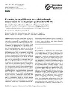
There were a total of 8300 atmospheric profiles used for the simulations in this work. The profiles are derived from Met Office’s numerical weather prediction model. For a description of the Met Office numerical weather prediction profiles at high altitude and a list of assimilated data, see Long et al. (2013). The profiles are abstractly shown in Fig. 1. Note that there is an unfortunate visual illusion in Fig. 1 that there is a discontinuity between the temperature at the 10 Pa level (65 km) and the temperature at higher pressure levels. One major problem we encounter is that the channels of SSMIS Atmos. Meas. Tech., 9, 841–857, 2016
844
R. Larsson et al.: High altitude SSMIS: radiative transfer model comparison for NWP Atmospheric profiles
10-1
Pressure [Pa]
100 101 102 103 104 105 150 160 170 180 190 200 210 220 230 240 250 260 270 280 290 300
Temperature [K]
Figure 1. The atmospheric profiles used in this study. The horizontal lines are profile levels and color scale is normalized per profile level: darker regions in the figure indicate more profiles with that temperature.
the models differ for the higher channels 19 and 20. This discussion focus on qualitative differences between the models that are apparent for the channels despite the otherwise unrealistic simulations. As one more note on the atmospheric profiles, we assume, for simplicity, that there is a constant molecular oxygen volume mixing ratio for the entire profile even though this is not the case above ∼ 80 km. Version 11 of the International Geomagnetic Reference Field (IGRF-11; Finlay et al., 2010) is used for the ARTS simulations with a three-dimensional magnetic field. The two-dimensional magnetic field values at the altitude corresponding to 5 Pa (around 70 km) have been extracted from IGRF-11 for both ARTS and RTTOV for those simulations. These extracted values are mapped in Fig. 2, which also shows the global coverage of the data sets. The argument for using a two-dimensional magnetic field is that the magnetic field does not change much along the path of a transfer. If this argument is good for SSMIS observations, then the difference in brightness temperature as a function of magnetic field extraction altitude will be small for the simulations. 2.3
are sensitive to altitudes that are above the numerical weather prediction profiles’ top at 10 Pa. The weighting functions of channels 21 and 22 are mostly covered by the 10 Pa level but the weighting functions of channels 19 and 20 are not covered. To work around the problem of insufficiently highreaching pressure levels of the Met Office profiles, we assume that all higher altitude pressure levels have the same temperature as the 10 Pa level. This assumption is simple and inaccurate, as the lapse rates at high altitudes are generally large, but it is another work altogether to define how to deal with the temperature field above the top of the numerical prediction profiles in a way that minimizes errors. One reason to use a constant temperature extrapolation for this work follows from the fact that RTTOV predicts optical depths on preset coefficient levels. When presented with an atmosphere that has insufficiently high-reaching pressure levels, RTTOV does this after assigning the temperature of the supplied atmospheric top to all the overlying coefficient levels, which is an extrapolation at constant temperature across the overlying layer of gas. The radiative transfer integration is performed subsequently on the supplied levels, but includes the source function and the absorption for the overlying layer of gas by, in effect, moving the supplied top at fixed temperature across this layer to represent the space boundary. Since the radiation of both channels 21 and 22 is mostly emitted at an altitude range covered by the Met Office atmospheric profiles, forcing a constant temperature above the top emulates the behavior of RTTOV when it is directly supplied by the Met Office profiles for these channels. This still means that the simulated results of channels 19 and 20 are unrealistic. We therefore favor the low-altitude channels 21 and 22 in this comparison work but include a brief discussion on how Atmos. Meas. Tech., 9, 841–857, 2016
Spectroscopic considerations
The RTTOV simulations have been performed with the prediction coefficients derived by Han et al. (2007) in this study. ARTS uses line center frequencies from the Jet Propulsion Laboratory spectroscopy database (http://spec.jpl.nasa.gov/). There is a mismatch between the input line centers to ARTS and RTTOV by exactly 8.4, 8.1, 8.9, and 8.2 kHz referring to Table 1 in Han et al. (2007) for the 7+, 9+, 15+, and 17+ O2 lines, respectively. ARTS always uses the higher frequency. The line centers given by, e.g., Tretyakov et al. (2005) are 2.2, 1.9, 5.1, and 7.4 kHz below the line centers used by ARTS, but were derived for use at low altitudes where pressure broadening is more important than exactness of line centers. Nevertheless the model input spectroscopy is similar and should be compared with the frequency stability of SSMIS reported by Kunkee et al. (2008) (80 kHz for channels 19, 20, and 21; 120 kHz for channel 22). Since the frequency instabilities are larger than differences in the lines’ central frequencies between the models, we do not think that line center accuracy is crucial for the comparison with SSMIS data, but it can still introduce biases between the models. The channels’ spectral response and a few examples of the simulated spectra from ARTS can be seen in Fig. 3. (Note that from code review at the Met Office for the derivation of RTTOV’s coefficients, we find that it appears that round-off levels of 100 kHz have been used for the line centers. The resulting differences in line centers between ARTS and RTTOV are still small compared to SSMIS frequency stability. They are instead 16, 32, 14, and −26 kHz for the 7+, 9+, 15+, and 17+ lines, respectively.) From Fig. 3, we see that channels 19 and 20 are in the center of the broadened lines, and that channels 21 and 22 are in the line shape’s wings near the equator (weak magwww.atmos-meas-tech.net/9/841/2016/
R. Larsson et al.: High altitude SSMIS: radiative transfer model comparison for NWP
845
Table 1. Mean and standard deviations of our comparison for the four SSMIS channels. The left two columns with data are a direct comparison between the SSMIS data set and the corresponding full model simulations. The rightmost column shows the Zeeman effect by turning the effect on and off in ARTS. The remaining columns compare RTTOV simulations with ARTS simulations using three-dimensional and two-dimensional magnetic fields. SD denotes standard deviation. n/a denotes data that are not applicable. Noise levels are from Kunkee et al. (2008). Channel 19
20
SSMIS cf. Full ARTS RTTOV
Mean SD Noise
n/a n/a
Mean SD Noise
n/a n/a
RTTOV cf. 3-D mag. ARTS 2-D mag. ARTS
Zeeman Effect
n/a n/a
−0.336 K 1.8305 K
−0.110 K 0.3304 K
−0.435 K 2.8931 K
n/a n/a
−0.068 K 1.7340 K
0.1668 K 0.2679 K
−2.244 K 1.9820 K
2.7 K
2.7 K
21
Mean SD Noise
−0.344 K −1.275 K 2.4362 K 2.4462 K 1.9 K
−0.931 K 0.5530 K
−0.921 K 0.5676 K
−3.125 K 1.8862 K
22
Mean SD Noise
−0.628 K −1.156 K 1.3750 K 1.4023 K 1.3 K
−0.528 K 0.2437 K
−0.532 K 0.2428 K
0.1285 K 0.0875 K
Figure 2. Magnetic field used in our simulation mapped on a two-dimensional surface showing the strength of the field in the left panel. The right panel contains the angle between the magnetic field vector and the radiation’s propagation path. (This figure appears in Larsson (2014) and is republished with rights from EUMETSAT.)
netic field strengths), but that channel 21 is on the edge of the strongly Zeeman-affected part of the line when the magnetic field is stronger (i.e., near the poles). It is clear from this figure in combination with Fig. 2 that the increased magnetic field strength at higher latitudes causes a stronger broadening of the line. Since the SSMIS channels measure so close to the line centers, resulting errors from line center mismatches have been studied using the same simulations as shown in Fig. 3. The results of these tests are in Fig. 4, which shows ARTS simulations with uniformly shifted line centers (emulating a channel frequency shift). We see that the effect of the channel frequency shift is large for channels 19 and 20 near the equator (1Tb ≈ ±2 K at ±50 kHz shift looking westward) and that the effect here strongly depends on the observational geometry (1Tb ≈ ±2 K at 50 kHz shift when instead looking eastward). Closer to the North Pole, the effect is still
www.atmos-meas-tech.net/9/841/2016/
noticeable but is fairly constant with observational geometry (1Tb ≈ −0.1 K at ±50 kHz). There is a noticeable effect on channel 21 of 1Tb ≈ ±0.5 K at ±50 kHz for the polar simulations and 1Tb ≈ ±0.2 K at ±50 kHz for equatorial simulations. Channel 22 is only weakly affected by a shifting channel center, with |1Tb | < 0.05 K even at ±150 kHz shift. Note that Figs. 3 and 4 only represent two locations on the globe and that the absolute effect of a shifting channel center changes over the globe. Finally, we have prepared weighting functions for an example of one orbit (the orbit is from 1 January 2012 around 13:30 UTC) and for two measurement pixels (or observational geometries that are relative to the motion of the satellite). These are shown in Fig. 5. With respect to each channel, the weighting function of channel 22 is almost constant over the orbit and observational geometry is not im-
Atmos. Meas. Tech., 9, 841–857, 2016
846
R. Larsson et al.: High altitude SSMIS: radiative transfer model comparison for NWP O2 9+ line 280
260
260
240
220
200
180
60.4296
60.4348 Frequency [GHz]
Eq. East Eq. West Po. East Po. West Ch 20 Ch 21 Ch 22 60.44
Brightness [K]
Brightness [K]
O2 7+ line 280
240
220
200
180
61.1454
O2 17+ line
270
270
260
260
250
250 Brightness [K]
Brightness [K]
O2 15+ line
240 230 220
240 230 220
210 200
61.1506 Frequency [GHz]
Eq. East Eq. West Po. East Po. West Ch 20 Ch 21 Ch 22 61.1557
62.9959
62.998 Frequency [GHz]
Eq. East Eq. West Po. East Po. West Ch 19 63.0001
210 200
63.5664
63.5685 Frequency [GHz]
Eq. East Eq. West Po. East Po. West Ch 19 63.5706
Figure 3. Channel configurations for SSMIS. The colors represent polar simulations (60◦ N 0◦ E; teal and red lines) and equatorial simulations (0◦ N 0◦ E; blue and green lines). The different colors also denote the simulations’ azimuthal angle; blue and red responses show SSMIS facing towards the east (75◦ ), whereas green and teal show it facing towards the west (−75◦ ). The channels are indicated by black boxes of different line styles as seen in the legends. The simulated measurement responses are assumed to be the average of the spectra within the frequency ranges.
portant. Channel 21 is similarly little influenced by observational geometry but in the polar region (the reader should be reminded that this is where the magnetic field is stronger) the weighting function is “smeared” and the channel is influenced by much greater altitudes (though the influence is not very strong). Both of the weighting functions of channels 19 and 20 change with geographical location and with observational geometry. It can be seen that the observational geometry is important by the broadened weighting function in the westward-facing pixel as compared to the along-thetrack pixel around the first pass at −30◦ latitude, which is not as evident during the second pass (comparing the then eastward-facing pixel to the along-the-track pixel). Again, remember that Fig. 5 only shows an example of one orbit and that the weighting function will be different for other orbits and for other observational geometries. 2.4
Are there layering issues?
Since ARTS averages optical properties and RTTOV averages atmospheric properties to create the layer transfer, we must quantify the errors introduced by this model discrepancy. We do this by artificially decreasing the maximum layer Atmos. Meas. Tech., 9, 841–857, 2016
thickness (ri of Eq. 4) for ARTS. We find that using an atmospheric layering of 50 m for a few of the profiles instead of using the same layering thickness as RTTOV only changes our results by ∼ 2 × 10⁻⁴ K. The layering thickness is therefore not an issue for ARTS. We cannot test this for RTTOV directly without altering the predictor coefficients, but it is shown by Han et al. (2007) that using a sparsely layered approach or using a 1 km altitude grid does not alter the simulated brightness temperature much. From these observations we argue that there is no issue with the layers in the present study.
3
Results and discussions
The results of our comparison are summarized in Table 1. Channel-by-channel, the table shows the mean differences between the compared data sets, their corresponding standard deviations, and the channels’ noise equivalent temperatures. Figures 6 to 9 show the data sets in spread plots and as global distribution maps for channels 19 to 22. Figure 10 shows SSMIS measurements cf. the simulations for channel 21, and Fig. 11 shows SSMIS measurements cf. the simulations for www.atmos-meas-tech.net/9/841/2016/
R. Larsson et al.: High altitude SSMIS: radiative transfer model comparison for NWP
4 3 2 1 0 −1 −2 Eq. East Eq. West Po. East −4 Po. West −150 −100 −50 0 50 100 150 Channel frequency shift [kHz] −3
Brightness temperature change [K]
Brightness temperature change [K]
Channel 19 5
Channel 20
7 6 5 4 3 2 1 0 −1 −2 −3 −4 −5
0.2 0 −0.2 −0.4 −0.6 −0.8 Eq. East Eq. West Po. East Po. West −150 −100 −50 0 50 100 150 Channel frequency shift [kHz] −1
−1.2
Channel 22 Brightness temperature change [K]
Brightness temperature change [K]
Channel 21 0.4
0.03 0.02 0.01 0 −0.01 −0.02
Eq. East Eq. West Po. East −0.03 Po. West −150 −100 −50 0 50 100 150 Channel frequency shift [kHz]
Figure 4. Changes in brightness temperatures introduced by an offset in channel frequency for a single atmospheric scenario. This figure shows the changes in channel brightness temperatures for the simulations in Fig. 3; both legends and line colors represent the cases in Fig. 3. The 0 kHz brightness temperature has been used as reference (hence 0 K at 0 kHz). The title of each subplot shows the channel.
channel 22. Figure 12 has been prepared to show the Zeeman effect in ARTS for all channels and Fig. 13 has been prepared to interpret equatorial results more easily. 3.1
angular dependencies of the Zeeman effect near the equator. Especially clear perhaps above the Atlantic between Brazil and western Africa, the center of the measurement swaths around the equator is less influenced by the Zeeman effect than the surrounding swath positions. 3.1.1
Eq. East Eq. West Po. East Po. West −150 −100 −50 0 50 100 150 Channel frequency shift [kHz]
Model to model
Before comparing RTTOV and ARTS we will discuss Fig. 12. The figure shows the model effect of turning the magnetic field on and off in ARTS. By comparing to Fig. 2, we see that there is an anti-correlation between magnetic field strength and brightness temperature change for channels 19, 20, and 22. The correlation for channel 21 is instead positive. On a channel-by-channel basis, channel 22 experiences minimal Zeeman effect. In the extreme polar regions, the channel is only up to 0.4 K Tb warmer when the Zeeman effect is considered, but most of the rest of the planet experiences a Zeeman effect that is less than 0.1 K Tb . Channel 21 experiences the absolute strongest Zeeman effect out of all channels of just above 8 K Tb at the strongest sources of magnetic fields. The weaker magnetic field regions only experience around 1 or 2 K Tb . The simulations for channels 19 and 20 change a lot when the Zeeman effect is considered. Channel 20 gets 2 K Tb warmer at strong magnetic sources with the Zeeman effect considered. The same value for channel 19 is higher, at 5 K Tb . Both channels are around 7 K Tb colder at the equator. One interesting feature to note is the www.atmos-meas-tech.net/9/841/2016/
847
Channels 19 and 20
Figure 6 shows the channel 19 comparison of RTTOV with ARTS, which was run using both a full three-dimensional magnetic field and an identical two-dimensional magnetic field setup as used by RTTOV. From Table 1, it can be seen that the mean brightness temperature differences between the models are small on average regardless of magnetic field setup, with both comparisons’ mean difference showing |1Tb | < 0.34 K. This is about the same size as the average Zeeman effect in ARTS at 1Tb ≈ −0.44 K. There is a large increase in the standard deviation of the differences from 0.33 K in the two-dimensional magnetic field comparison to the three-dimensional magnetic field comparison, which has a standard deviation of 1.8 K. There is a still larger increase in standard deviation to 2.9 K if the Zeeman effect is ignored. From the global distribution maps shown in Fig. 6, we see that the largest discrepancies for channel 19 between RTTOV and ARTS with a three-dimensional magnetic field are located all across the equator, with a brightness temperature differences of up to 7 K systematically distributed in higher and lower brightness temperature regions; most warmer regions are located to the south of the equator and most colder regions are located to the north of the equator when the satellite is moving southward. When the satellite is moving northward, the resulting warm–cold region distribution seems to change across the swath. By remembering Fig. 2, which shows the two-dimensional magnetic field, we can by eye correlate these larger brightness temperature differences with areas of relatively weak magnetic field strength and with a magnetic field angle that is close to being parallel with the radiation path. We use Fig. 13 to focus on equatorial differences between the channels in this study. For channel 19, this figure shows that the differences between three-dimensional ARTS and RTTOV range over 7 K near the equator, but that the same range for differences between two-dimensional ARTS and RTTOV is only around 1 K. We note that a large change over the swath is consistent with the changing weighting functions of channel 19 in Fig. 5, which close to the equator can be quite broadened by changing the observational geometry. Thus, if the satellite had been moving northward over Eurasia, instead of over the Pacific Ocean, we cannot expect to see the same type of regional discrepancies since the magnetic field angle is changed by the viewing geometry. Looking only at the comparison of RTTOV and ARTS simulations with a two-dimensional magnetic field for channel 19, we find brightness temperature differences between the models of up to 1 K. There appears to Atmos. Meas. Tech., 9, 841–857, 2016
848
R. Larsson et al.: High altitude SSMIS: radiative transfer model comparison for NWP
Figure 5. Weighting functions for SSMIS from ARTS with a three-dimensional magnetic field for an example of one orbit for channels 19 to 22. Color shows the change in transmissions per kilometer of atmospheric altitude traversed by the radiation. The y axis is the altitude range and the x axis shows the latitude of the sensor as a function of time. For all four channels, two swath positions are shown. Position no. 15 points downward along the orbit of the sensor. Position no. 1 points westward as the sensor travels northward, and it points eastward as the sensor travels southward.
be a weak positive bias of around 0.3 K in the equatorial regions and a weak negative bias of around 0.6 K closer to the poles. We cannot identify the reason for these discrepancies clearly but the line center frequency differences of around 20 kHz between the models can explain some of these differences. For channel 20 in Fig. 7, most of the same features are available as for channel 19 in Fig. 6, with a few modifications. From Table 1, the average brightness temperature differences between models are small, with both comparisons showing a mean of |1Tb | < 0.17 K. The average model to model difference is thus much smaller than the average Zeeman effect in ARTS, which is 1Tb ≈ −2.2 K. The standard deviation of the model to model differences changes in the same way for channel 20 as it does for channel 19. RTTOV simulations minus ARTS simulations with a threedimensional magnetic field have a much larger standard deviation of 1.7 K than the standard deviation of 0.27 K for RTTOV simulations minus ARTS simulations with a twodimensional magnetic field. For channel 20 the ARTS Zeeman effect standard deviation of 2.0 K is relatively close to the three-dimensional model to model standard deviation. From Fig. 13, it can be seen that the equatorial differences between three- and two-dimensional ARTS and RTTOV are similar to the differences for channel 19. One interesting difference is that while channel 19 has a fairly even equatorial bias when it compares two-dimensional ARTS to RTTOV simulations, this is not the case for channel 20. Instead, the eastern hemisphere experiences a positive bias of about 0.5 to 0.7 K and the western hemisphere sees close to no biases.
Atmos. Meas. Tech., 9, 841–857, 2016
The errors that remain in the comparison with RTTOV and ARTS simulations with a two-dimensional magnetic field for channel 20 are similar to those for channel 19 of up to ∼ 1.5 K. Because both line centers for channel 20 are shifted in frequency with the same sign, we can compare the remaining discrepancies in Fig. 7 to the channel frequency shift presented in Fig. 4. As a test not presented in any figures of this work, we ran ARTS with changed line center frequencies of 30 kHz for the lines influencing channel 20. This altered spectroscopy reduces the mean difference between the models by half, but the standard deviation still remains fairly unchanged. This means that there are still unidentified discrepancies between the models for channel 20. 3.1.2
Channels 21 and 22
Common to both the lower peaking channels 21 and 22 is that the reduction to a two-dimensional magnetic field in ARTS is numerically noticeable but much smaller than for channels 19 and 20. It is possible in Fig. 8, for channel 21, to see this difference qualitatively in the global distributions near magnetically strong regions. One example is above Siberia where there is a region with two-dimensional ARTS simulations that are 1Tb ≈ 0.1 K warmer than RTTOV. The threedimensional ARTS simulations are instead 1Tb ≈ −0.2 K to RTTOV. It is also possible to see a systematic 1 K gradient over the swaths near the equator in the comparison of RTTOV and three-dimensional ARTS in Fig. 13 for channel 21. This systematic gradient is reduced to a fraction of a Kelvin for differences between two-dimensional ARTS and RTTOV. Similarly to channels 19 and 20, these swath discrepancies www.atmos-meas-tech.net/9/841/2016/
R. Larsson et al.: High altitude SSMIS: radiative transfer model comparison for NWP
849
Figure 6. Channel 19 comparison of RTTOV and ARTS simulations. The upper row contains spread plots for RTTOV simulations on the y axis and for ARTS simulations on the x axis. The lower row contains the above spread plots mapped onto the surface of Earth to where the corresponding SSMIS measurement was done. In these maps, the magnitudes of the difference between the simulations are shown in color. The color corresponds to ARTS minus RTTOV. The left column shows RTTOV compared to ARTS simulations with a three-dimensional magnetic field and the right column shows RTTOV compared to ARTS simulations with a two-dimensional magnetic field. It is important to note that the color scale changes between the maps; this has been done to highlight all model differences, which are discussed in the text.
should change when SSMIS is scanning northward or southward. Still, since the Zeeman effect is weak for channel 21 at the equator, most model differences there (the average bias is around 1.7 K in Fig. 13) are due to other reasons than the Zeeman effect. Focusing only on two-dimensional magnetic field simulations for channel 21 (Fig. 8; right column), the polar regions agree fairly well between ARTS and RTTOV, with |1Tb | < 0.6 K, barring a −1 K region above Antarctica close to 0◦ E longitude. These < 0.6 K differences are possible to understand from the 30 kHz line shifts identified for channel 20 above. Similarly to channel 20, however, introducing the line center shifts only reduces the model to model discrepancies, without much change in the standard deviation. (We remind the reader that channels 20, 21, and 22 measure the same two lines as are shown in Fig. 3; therefore, effects on one of the channels should be similar to the others.) Since channel 21 weighting functions of Fig. 5 are stretched to higher altitudes near the poles, it is possible that some model differences have been missed or exaggerated in our study due to our constant temperature profiles at these higher altitudes. It is deemed unlikely that this has had a big impact on our results because the largest differences between the models
www.atmos-meas-tech.net/9/841/2016/
are found across the equator, where the channel 21 weighting function is covered by our physical profile. Also, the standard deviation of the model to model difference is about 0.56 K. In relation to the sensor noise equivalent temperature of 1.9 K, the model to model standard deviation is small, so any effect of the stretched weighting function on our comparison is also small. From Fig. 12, the Zeeman effect is up to 8 K Tb at the strong magnetic regions for channel 21, whereas the models compare to within 0.6 K in these regions. This means that the models are still fairly close to one another in the strong magnetic field regions compared to the size of the Zeeman effect. Instead of at the poles, the largest model differences are found close to the equator, where differences of almost 3 K appear. We cannot explain these large differences from the channel shifts of Fig. 4. For channel 22, there seems to be no correlation between magnetic field parameters and model to model differences. This is not surprising considering that the Zeeman effect is not very important for channel 22, with an average effect of 1Tb = 0.13 K that has a standard deviation of only 0.088 K. The mean differences between the models are 1Tb ≈ −0.53 K with a standard deviation of 0.24 K, regardless of magnetic field setup in ARTS. Concerning channel 21,
Atmos. Meas. Tech., 9, 841–857, 2016
850
R. Larsson et al.: High altitude SSMIS: radiative transfer model comparison for NWP
Figure 7. Channel 20 comparison of RTTOV and ARTS simulations as for Fig. 6.
Figure 8. Channel 21 comparison of RTTOV and ARTS simulations as for Fig. 6 but with a fixed color scale.
Atmos. Meas. Tech., 9, 841–857, 2016
www.atmos-meas-tech.net/9/841/2016/
R. Larsson et al.: High altitude SSMIS: radiative transfer model comparison for NWP
851
Figure 9. Channel 22 comparison of RTTOV and ARTS simulations as for Fig. 6 but with a fixed color scale.
we find from Fig. 13 that near the equator there is a larger than average negative bias. For channel 22 it averages at 1Tb ≈ −0.75 K. Another region of interest is the South Pole, where the largest model to model differences occur – it is not shown in any plots that Antarctica is the warmest region in our simulations with atmospheric temperature of around 280 K for channel 22. From the scatter plots of Fig. 9, we see that there are beginnings of deviation between the models at higher temperatures, which show the Antarctica deviations. One potential cause for these discrepancies is therefore that the RTTOV coefficients were derived using transmission coefficients from simulations with an atmospheric training set that also had highest temperatures around 280 K at the peak of the weighting function of channel 22. It has previously been identified as a problem by Buehler et al. (2006) for water spectroscopy models that RTTOV coefficients derived for atmospheric input close to the limits of the training set can cause accuracy issues in RTTOV. In other regions, the model to model differences are small and appear to oscillate around 0 K. 3.2
Models to measurements
Direct comparison of simulated measurements with the SSMIS data set is only possible for channels 21 and 22 because the higher altitude channels 19 and 20 are not covered by the altitude levels of the numerical weather prediction profiles. We want to remind the reader that the Met Office numerical www.atmos-meas-tech.net/9/841/2016/
weather prediction model profiles are believed to be inaccurate at higher altitudes. All such inaccuracies are retained in the following comparisons of models to measurements. The comparisons for channel 21 between SSMIS measurements, with regards to RTTOV simulations and with regards to ARTS simulations with a three-dimensional magnetic field, are found in Fig. 10. We find that the mean value of SSMIS measurements minus RTTOV simulations is −1.3 K, and the mean value of SSMIS measurements minus ARTS simulations is −0.34 K. ARTS agrees better than RTTOV with SSMIS. Both comparisons have a standard deviation of around 2.4 K, and the noise equivalent temperature of the sensor is 1.9 K (Kunkee et al., 2008). So even if ARTS appears to be better, RTTOV simulations are close to SSMIS measurements given the sensor’s noise and RTTOV is close to ARTS given the simulations to measurement standard deviations. One key point that we want to take note of is that the noise of channel 21 is a lot smaller than the standard deviation of simulations to measurement. This is a similarity between our study and the one performed by Han et al. (2007). They found that RTTOV agrees with SSMIS at a root mean square of 2.3 K at a mean difference of −0.95 K for channel 21. Han et al. (2007) use retrieved temperature profiles by the limb-scanning SABER instrument on board the TIMED satellite. This should mean that their temperature profiles are reasonably accurate, since limb scanners have a high signalto-noise ratio. Still, they found, as we do, that the standard Atmos. Meas. Tech., 9, 841–857, 2016
852
R. Larsson et al.: High altitude SSMIS: radiative transfer model comparison for NWP
Figure 10. Comparison of model simulations and SSMIS measurements for channel 21. Similar to Fig. 6 with some changes. The left column spread plot still shows RTTOV simulations on the y axis but SSMIS measurements on the x axis; the corresponding scatter map represents SSMIS minus RTTOV. The right column spread plot shows ARTS simulations with a three-dimensional magnetic field on the y axis and SSMIS measurements on the x axis; the corresponding scatter map is for SSMIS minus ARTS.
deviation of the simulations to measurement are consistently larger than the noise of the sensor. Looking in more details at the global distribution maps, we see that the largest discrepancies for both models are available closer to the poles, with a tendency for warmer brightness temperature differences (up to about 7 K) in the south and colder brightness temperature differences in the north (down to about −7 K). The weighting function of channel 21 is shifted upwards for stronger magnetic field (see Fig. 5 at high absolute latitudes). This upwards shift places a significant part of the weighting function at pressure levels where we have set the temperature to a constant value (above the 10 Pa/65 km level). Clearly a better method for extending the temperatures above 10 Pa is required. Across the equator the models are closer to SSMIS measurements. RTTOV agrees better with SSMIS measurements near the equator, with an average difference of around −1 K, than ARTS simulations, which has an average difference of 2 K to the SSMIS measurements. Looking at the equator in more details in Fig. 13, we cannot determine if ARTS or RTTOV equatorial behavior is best there for channel 21. Both models compare to SSMIS with much larger effects over the swath at the equator than how the models compare to one another. Swath effects are about 3 K large between models and measurements. We remind the reader that these swath effects are 1 K between Atmos. Meas. Tech., 9, 841–857, 2016
three-dimensional ARTS and RTTOV. ARTS has on average slightly smaller swath effects – reduced by about 20 % judging by differences in the absolute averages of the a regression coefficient in the linear fit of y = a x + b that is plotted – than RTTOV but there is a large variation in these swath effects. There are some similarities between the channel 21 and the channel 22 comparisons of model simulations and SSMIS measurements as found in Fig. 11. In average, ARTS still agrees better than RTTOV with SSMIS measurements, with the respective differences to measurements being 1Tb ≈ −0.63 K for ARTS and 1Tb ≈ −1.3 K for RTTOV as seen in Table 1. Both models have approximately 1.4 K standard deviation to the measurements, which is similar to the sensor equivalent noise temperature of 1.3 K (Kunkee et al., 2008). Since the model-to-measurement standard deviation retains atmospheric input errors, this means that the models have a good agreement with the measurements. There are still a few dominating features visible in the global distribution maps. These features are all in the Southern Hemisphere, with a region above West Antarctica that has a −7.5 K bias compared to both models, and two regions with a 3 K bias to the observations, one located just north of the cold Antarctica anomaly and another located towards the east of it. We note that RTTOV and SSMIS agree better for channel 22 in our study than in the study by Han et al. (2007). www.atmos-meas-tech.net/9/841/2016/
R. Larsson et al.: High altitude SSMIS: radiative transfer model comparison for NWP
853
Figure 11. Comparison of model simulations and SSMIS measurements for channel 22 as for Fig. 10.
Figure 12. The Zeeman effect in ARTS for all four channels. Colors correspond to ARTS without any magnetic field minus ARTS with a three-dimensional magnetic field.
They found approximately the same average difference between RTTOV and SSMIS as we did (1Tb ≈ −1.3 K), but the standard deviation in their test was much larger at 2.2 K compared to 1.4 K in ours. The temperature profiles are more accurate for limb sounding, so their uncertainties should reasonably be below or similar to ours. One possible explanation is that there are measurements with colder brightness www.atmos-meas-tech.net/9/841/2016/
temperatures included in the study by Han et al. (2007) than compared to our study. These lower brightness temperatures were consistently underestimated by RTTOV, which should increase the standard deviation.
Atmos. Meas. Tech., 9, 841–857, 2016
R. Larsson et al.: High altitude SSMIS: radiative transfer model comparison for NWP
Latitude
854
20 10 0 −10 −20 −150
−100
Channel 19
10
0 Longitude
−50 Channel 20
8
50
100
Channel 21
Channel 22
4 2 0 −2 −4 −6
50 −150 −100 −50 0 Longitude
6 4 2 0 −2 −4 −6
100 150
50 −150 −100 −50 0 Longitude
Channel 19
−1.0
−1.5
−2.0
−2.5
−3.0
100 150
−0.2 RTTOV cf. 3D mag. ARTS [K]
6
RTTOV cf. 3D mag. ARTS [K]
RTTOV cf. 3D mag. ARTS [K]
RTTOV cf. 3D mag. ARTS [K]
−0.5
8
Channel 20
50 −150 −100 −50 0 Longitude
0.0
100 150
50 −150 −100 −50 0 Longitude
Channel 21
−1.2 −1.4 −1.6 −1.8 −2.0 −2.2
4
2 1 0 −1 −2
3D mag. ARTS cf. SSMIS [K]
3
3
−2.4
100 150
Channel 21
4
RTTOV cf. SSMIS [K]
3D mag. ARTS cf. SSMIS [K]
0.5
50 −150 −100 −50 0 Longitude
100 150
−0.3 −0.4 −0.5 −0.6 −0.7 −0.8 −0.9 −1.0
−0.5 50 −150 −100 −50 0 Longitude
4
−1.0
Channel 22
2 1 0 −1 −2
−1 −2
−4
−4
50 −150 −100 −50 0 Longitude
100 150
Channel 22
3
0
−4
100 150
4
1
−3
50 −150 −100 −50 0 Longitude
Channel 22
2
−3 100 150
−1.1
100 150
3
−3 50 −150 −100 −50 0 Longitude
50 −150 −100 −50 0 Longitude
RTTOV cf. SSMIS [K]
−0.5
−0.8
−0.2 RTTOV cf. 2D mag. ARTS [K]
0.0
−0.6
Channel 21
1.0
RTTOV cf. 2D mag. ARTS [K]
RTTOV cf. 2D mag. ARTS [K]
RTTOV cf. 2D mag. ARTS [K]
0.5
−0.4
−1.2
100 150
−1.0 1.0
150
2 1 0 −1 −2 −3
50 −150 −100 −50 0 Longitude
100 150
−4
50 −150 −100 −50 0 Longitude
100 150
Figure 13. The swath dependencies around the equatorial crossings of this study. The first row shows the map of the data. Color-coding is the same in this map as in the other plots where the swath from one orbit has its own colors; black circles are not used because they are more than 5◦ from the equator (5◦ was just arbitrarily chosen as the limit). The y axis label in the other plots overlap with labels in Figs. 6 to 11. Channels are named in the plot titles. Linear regression for brightness temperature differences was performed over longitude and the best-fit line is drawn between ±20 % of the longitude range of the data from each orbit. The first two rows of the regression plots represent the model comparison and the last row represents the comparison between the models and SSMIS measurements.
4
Summary, conclusions, and outlook
We have presented a comparative study showing how well the fast RTTOV agrees with reference model ARTS for the high-altitude channels 19–22 of SSMIS using globally distributed numerical weather prediction model profiles from Met Office. This study shows that the RTTOV Zeeman effect scheme for SSMIS implemented by Han et al. (2007) works well. The agreement between the forward simulations and Atmos. Meas. Tech., 9, 841–857, 2016
the corresponding SSMIS measurements is generally good but there are some discrepancies; quantitative values of the comparison are summarized in Table 1. We conclude, when comparing ARTS to RTTOV, that using a three-dimensional magnetic field in ARTS gives an increased standard deviation compared to using a twodimensional magnetic field in ARTS for channels 19 and 20; this increase is from 0.3 to 1.8 K for channel 19 and from 0.27 to 1.7 K for channel 20. The brightness temperature
www.atmos-meas-tech.net/9/841/2016/
R. Larsson et al.: High altitude SSMIS: radiative transfer model comparison for NWP differences by a three-dimensional magnetic field for these channels are found to be up to ±7 K across the equator, whereas ARTS with a two-dimensional magnetic field is in the range ±1 K from RTTOV. Since we follow the numerical weather prediction profile top (and emulate the behavior of RTTOV above this top), we cannot be sure that these are the model differences for a proper atmosphere. Despite this limitation, our comparisons still suggest that the dimensionality of the magnetic field is important for the higher altitude channels. The natural top of the mesosphere variability is around 15 K, so potential modeling errors of up to 7 K is a lot; however, we have not yet tested how this translates to numerical weather prediction model errors at these altitudes. Today, the estimated numerical weather prediction model errors are about 10 K at these altitudes. These errors will be reduced by using RTTOV with two-dimensional magnetic fields and the information available in the higher altitude SSMIS channels, but we cannot estimate by how much – this must be tested using the present version of RTTOV in trial operational settings. Still, it would be better to use a three-dimensional magnetic field in RTTOV than a two-dimensional magnetic field but a fast Zeeman scheme using a three-dimensional magnetic fields is not yet available. It is difficult to update RTTOV for three-dimensional magnetic fields but it should be possible. The coefficients used in RTTOV are generated from a large set of calculations that fits the effective scalar line-by-line transmission to space (Eq. 2) to a predetermined set of predictors. The polarized transmission from a level to space depends on the polarized transmission across all levels closer to the sensor (through the Ts of Eq. 3). Therefore, using a three-dimensional magnetic field with the present set of predictors will not work, since changes at higher altitudes change the effective scalar transmission to space. We have not attempted to extend the present set of predictors to account for perturbations at higher altitudes and further study will be necessary on how to achieve this. Since the magnetic field is fairly slow changing (see Fig. 2 for an estimate), a level-by-level set of perturbations might be applied to transmittances on the right in Eq. (3), and predictors incorporated into RTTOV to simulate the effect of the perturbations on the left of Eq. (2). This would allow the user to perturb a fixed input field, as presently expected by RTTOV, into a field that varies along the radiation path. Similar brightness temperature differences as for channels 19 and 20 between two- and three-dimensional magnetic fields are present for channel 21 but these differences are much smaller in magnitude. In regions where the magnetic field is strong (closer to the poles), the dimensionality of the magnetic field can give differences of about 0.5 K in local regions. The Zeeman effect is up to 8 K in these high magnetic field strength regions, so the Zeeman effect treatment in the models still agrees fairly well for a strong magnetic field. Near the equator, the differences over a swath of measurement are found to be about 1 K large due to the dimensionality of the magnetic field, whereas the Zeeman effect itself www.atmos-meas-tech.net/9/841/2016/
855
is only 1 to 2 K large. However, there are other effects than the Zeeman effect that are important in the comparisons of the models. The model difference at the equator is on average 3 K, and this is larger than the difference between using a three- or two-dimensional magnetic field. We cannot identify the reason for these 3 K model differences. In comparing models to measurements, the range of error is about ±7 K Tb for channel 21. The errors of Met Office profiles are expected to be large at higher altitudes, so we do not expect models and measurements to agree better than this for now. Channel 22 is unaffected by the dimensionality of the magnetic field because it is mostly unaffected by the Zeeman effect; the channel experience at most only a few tenths of a Kelvin of the Zeeman effect. Other differences dominate model to model differences. As regard to channel 21, there is an unexplained brightness temperature difference across the equator. For channel 22 this difference averages to around −0.75 K. Also, there seems to be a limit in the temperature range for RTTOV’s training data that lowers RTTOV accuracy at the highest atmospheric temperatures. This is seen above Antarctica, creating a model to model bias of about 1 K for regions with the highest atmospheric temperature in this study. Except for localized large differences between models and measurement, the modeled channel 22 shows a good agreement with the measurements. Since channel 22 measures at lower altitude than channel 21, the Met Office profiles are more accurate and this is reflected in the better agreement with SSMIS measurements. Our results imply that RTTOV, with the new Zeeman scheme by Han et al. (2007), models the SSMIS data set with acceptable accuracy compared to sensor noise parameters of channels 21 and 22. This in turn shows that the concerns Kobayashi et al. (2009) raised on using RTTOV’s past Zeeman capabilities for data assimilation schemes are addressed in newer versions. We recommend that future iterations of numerical weather prediction software start using versions of RTTOV from version 10 and onwards for the assimilation of SSMIS channels 21 and 22. This would not improve much over using an older RTTOV version for channel 22, but it would greatly improve agreements for channel 21. If SSMIS channel 21 is modeled well by RTTOV it can be assimilated into the numerical weather prediction scheme and consequently help improve middle mesospheric temperatures. It is likely that model to model discrepancies for channel 21 can be reduced even more if the model top levels reached higher altitudes, since high-latitude weighting functions of channel 21 reach much higher altitudes than equatorial weighting functions; a level top at 0.01 Pa/100 km is also necessary for channels 19 and 20 to be modeled. The lack of a three-dimensional magnetic field in RTTOV is not ideal for channel 21 but neither is it a huge issue. Models and measurements differ by 7 K at the equator currently and threedimensional magnetic field makes only about 1 K difference for this channel. An option to work around the dimensionality problem currently is to apply biases, similar to those we Atmos. Meas. Tech., 9, 841–857, 2016
856
R. Larsson et al.: High altitude SSMIS: radiative transfer model comparison for NWP
find between ARTS and RTTOV in this work, to correct the simulated measurements in the assimilation schemes. Especially regional biases have to be described for the inversions to apply these biases. Uncertainties in the atmospheric temperature field of the numerical weather prediction model levels at high altitude are nevertheless currently large and consideration of the higher altitude SSMIS channels can help mitigate these uncertainties. As regards to an outlook, there is an ongoing effort to use ARTS for retrievals of atmospheric temperature profiles using all of the high-altitude SSMIS channels. The results of these efforts will be reported upon in future work. Acknowledgements. This work was partly funded by EUMETSAT grant number NWP_VS13_02, with report number NWPSAF-MOVS-049. The writing of this article mainly took place in Hamburg under a CliSAP stipend. The authors also want to acknowledge the communities that support, both by usage and development, the two radiative transfer simulators. Edited by: D. Cimini
References Anderson, G. P., Clough, S. A., Kneizys, F. X.., Chetwynd, J. H., and Shettle, E. P.: AFGL atmospheric constituent profiles (0– 120 km), Air Force Geophysics Laboratory, Hanscom Air Force Base, MA, USA, TR-86-0110, 1986. Buehler, S. A., Eriksson, P., Kuhn, T., von Engeln, A., and Verdes, C.: ARTS, the atmospheric radiative transfer simulator, J. Quant. Spectrosc. Ra., 91, 65–93, doi:10.1016/j.jqsrt.2004.05.051, 2005. Buehler, S. A., Courcoux, N., and John, V. O.: Radiative transfer calculations for a passive microwave satellite sensor: Comparing a fast model and a line-by-line mode, J. Geophys. Res., 11, D20304, doi:10.1029/2005JD006552, 2006. Eriksson, P., Buehler, S. A., Davis, C. P., Emde, C., and Lemke, O.: ARTS, the atmospheric radiative transfer simulator, Version 2, J. Quant. Spectrosc. Ra., 112, 1551–1558, doi:10.1016/j.jqsrt.2011.03.001, 2011. Finlay, C. C., Maus, S., Beggan, C. D., Bondar, T. N., Chambodut, A., Chernova, T. A., Chulliat, A., Golovkov, V. P., Hamilton, B., Hamoudi, M., Holme, R., Hulot, G., Kuang, W., Langlais, B., Lesur, V., Lowes, F. J., Lühr, H., Macmillan, S., Mandea, M., McLean, S., Manoj, C., Menvielle, M., Michaelis, I., Olsen, N., Rauberg, J., Rother, M., Sabaka, T. J., Tangborn, A., TøffnerClausen, L., Thébault, E., Thomson, A. W. P., Wardinski, I., Wei, Z., and Zvereva, T. I.: International Geomagnetic Reference Field: the eleventh generation, Geophys. J. Int., 183, 1216–1230, doi:10.1111/j.1365-246X.2010.04804.x, 2010. Han, Y., Weng, F., Liu, Q., and van Delst, P.: A fast radiative transfer model for SSMIS upper atmosphere sounding channels, J. Geophys. Res., 112, D11121, doi:10.1029/2006JD008208, 2007. Han, Y., van Delst, P., and Weng, F.: An improved fast radiative transfer model for special sensor microwave imager/sounder upper atmosphere sounding channels, J. Geophys. Res., 115, D15109, doi:10.1029/2010JD013878, 2010.
Atmos. Meas. Tech., 9, 841–857, 2016
Hartmann, G. K., Degenhardt, W., Richards, M. L., Liebe, H. J., Hufford, G. A., Cotton,M. G., Belivacqua, R. M., Olivero, J. J., Kämpfer, N., and Langen, J.: Zeeman splitting of the 61 Gigahertz Oxygen (O2 ) line in the mesosphere, Geophys. Res. Lett., 23, 2329–2332, doi:10.1029/96GL01043, 1996. Kobayashi, S., Matricardi, M., Dee, D., and Uppala, S.: Toward a consistent reanalysis of the upper stratosphere based on radiance measurements from SSU and AMSU-A, Q. J. Roy. Meteorol. Soc., 135, 2086–2099, doi:10.1002/qj.514, 2009. Kunkee, D. B., Poe, G. A., Boucher, D. J., Swadley, S. D., Hong, Y., Wessel, J. E., and Uliana, E. A.: Design and Evaluation of the First Special Sensor Microwave Imager/Sounder, IEEE T. Geosci. Remote, 46, 863–883, doi:10.1109/TGRS.2008.917980, 2008. Larsson, R.: The Zeeman effect implementation for SSMIS in ARTS v. RTTOV, EUMETSAT, NWPSAF-MO-VS-049, 2014. Larsson, R., Buehler, S. A., Eriksson, P., and Mendrok, J.: A treatment of the Zeeman effect using Stokes formalism and its implementation in the Atmospheric Radiative Transfer Simulator (ARTS), J. Quant. Spectrosc. Ra., 133, 445–453, doi:10.1016/j.jqsrt.2013.09.006, 2014. Lenoir, W. B.: Propagation of Partially Polarized Waves in a Slightly Anisotropic Medium, J. Appl. Phys., 38, 5283–5290, doi:10.1063/1.1709315, 1967. Lenoir, W. B.: Microwave Spectrum of Molecular Oxygen in the Mesosphere, JGR, 73, 361–376, doi:10.1029/JA073i001p00361, 1968. Liebe, H. J.: Modeling attenuation and phase of radio waves in the air frequencies below 1000 GHz, Radio Sci., 16, 1183–1199, doi:10.1029/RS016i006p01183, 1981. Long, D. J., Jackson, D. R., Thuburn, J., and Mathison, C.: Validation of Met Office upper stratospheric and mesospheric analyses, Q. J. Roy. Meteorol. Soc., 139, 1214–1228, doi:10.1002/qj.2031, 2013. Navas-Guzmán, F., Kämpfer, N., Murk, A., Larsson, R., Buehler, S. A., and Eriksson, P.: Zeeman effect in atmospheric O2 measured by ground-based microwave radiometry, Atmos. Meas. Tech., 8, 1863–1874, doi:10.5194/amt-8-1863-2015, 2015. Remsberg, E. E., Marshall, B. T., Garcia-Comas, M., Krueger, D., Lingenfelser, G. S., Martin-Torres, J., Mlynczak, M. G., Russel III, J. M., Smith, A. K., Zhao, Y., Brown, C., Gordley, L. L., Lopez-Gonzalez, M. J., Lopez-Puertas, M., She, C.-Y., Taylor, M. J., and Thompson, R. E.: Assessment of the quality of the Version 1.07 temperatureversus-pressure profiles of the middle atmosphere from TIMED/SABER, J. Geophys. Res., 113, D17101, doi:10.1029/2008JD010013, 2008. Rosenkranz, P. W. and Staelin, D. H.: Polarized thermal microwave emission from oxygen in the mesosphere, Radio Sci., 23, 721– 729, doi:10.1029/RS023i005p00721, 1988. Rothman, L. S., Gordon, I. E., Babikov, Y., Barbe, A., Benner, D. C., Bernath, P. F., Birk, M., Bizzocchi, L., Boudon, V., Brown, L. R., Campargue, A., Chance, K., Cohen, E. A., Coudert, L. H., Devi, V. M., Drouin, B. J., Fayt, A., Flaud, J.-M., Gamache, R. R., Harrison, J. J., Hartmann, J.-M., Hill, C., Hodges, J. T., Jacquemart, D., Jolly, A., Lamouroux, J., Roy, R. J. L., Li, G., Long, D. A., Lyulin, O. M., Mackie, C. J., Massie, S. T., Mikhailenko, S., Müller, H. S. P., Naumenko, O. V., Nikitin, A. V., Orphal, J., Perevalov, V., Perrin, A., Polovtseva, E. R., Richard, C., Smith, M. A. H., Starikova, E., Sung, K., Tashkun, S., Tennyson, J.,
www.atmos-meas-tech.net/9/841/2016/
R. Larsson et al.: High altitude SSMIS: radiative transfer model comparison for NWP Toon, G. C., Tyuterev, V. G., and Wagner, G.: The HITRAN2012 molecular spectroscopic database, J. Quant. Spectrosc. Ra., 130, 4–50, doi:10.1016/j.jqsrt.2013.07.002, 2013. Saunders, R., Matricardi, M., and Brunel, P.: An improved fast radiative transfer model for assimilation of satellite radiance observations, Q. J. Roy. Meteor. Soc., 125, 1407–1425, doi:10.1002/qj.1999.49712555615, 1999. Schwartz, M. J., Read, W. G., and Van Snyder, W.: EOS MLS Forward Model Polarized Radiative Transfer for Zeeman-Split Oxygen Lines, IEEE T. Geosci. Remote, 44, 1182–1191, doi:10.1109/TGRS.2005.862267, 2006. Stähli, O., Murk, A., Kämpfer, N., Mätzler, C., and Eriksson, P.: Microwave radiometer to retrieve temperature profiles from the surface to the stratopause, Atmos. Meas. Tech., 6, 2477–2494, doi:10.5194/amt-6-2477-2013, 2013.
www.atmos-meas-tech.net/9/841/2016/
857
Swadley, S. D., Poe, G. A., Bell, W., Hong, Y., Kunkee, D. B., McDermid, I. S., and Leblanc, T.: Analysis and Characterization of the SSMIS Upper Atmosphere Sounding Channel Measurements, IEEE T. Geosci. Remote, 46, 962–983, doi:10.1109/TGRS.2008.916980, 2008. Tretyakov, M. Yu., Koshelev, M. A., Dorovskikh, V. V., Makarov, D. S., and Rosenkranz, P. W.: 60-GHz oxygen band: precise broadening and central frequencies of fine-structure lines, absolute absorption profile at atmospheric pressure, and revision of mixing coefficients, J. Mol. Struct., 231, 1–14, doi:10.1016/j.jms.2004.11.011, 2005. Zeeman, P.: On the Influence of Magnetism on the Nature of the Light Emitted by a Substance, Astrophys. J., 5, 332–347, 1897.
Atmos. Meas. Tech., 9, 841–857, 2016