Modelization of Dynamic Soil-Structure Interaction Using ... - mediaTUM

Lehrstuhl für Baumechanik der Technischen Universität München

Modelization of Dynamic Soil-Structure Interaction Using Integral Transform-Finite Element Coupling

Josia Irwan Rastandi

Vollständiger Abdruck der von der Fakultät für Bauingenieur- und Vermessungswesen der Technischen Universität München zur Erlangung des akademischen Grades eines Doktor-Ingenieurs genehmigten Dissertation.

Vorsitzender

:

Univ.-Prof. Dr.-Ing. K.-U. Bletzinger

Prüfer der Dissertation : 1. Univ.-Prof. Dr.-Ing. H. Grundmann 2. Univ.-Prof. Dr.-Ing. H. Kreuzinger

Die Dissertation wurde am 09.10.2003 bei der Technischen Universität München eingereicht und durch die Fakultät für Bauingenieur- und Vermessungswesen am 14.11.2003 angenommen.

To my wife Stella and our little daughter, Jessica

Zusammenfassung Das Ziel dieser Arbeit ist eine zuverlässige Modellierung der Wellenausbreitung bei der BauwerkBodenwechselwirkung in der Strukturdynamik. Dazu gehört sowohl die ausreichende Erfassung der Verhältnisse in unmittelbarer Bauwerksumgebung (Nahbereich), als auch die zutreffende Beschreibung der Ausbreitungsvorgänge in die weitere Bauwerksumgebung (Fernbereich). Für den Fernbereich (Halbraum) werden Integraltransformations-methoden benutzt. Eine flexible Beschreibung der Verhältnisse in unmittelbarer Bauwerks-umgebung wird am besten durch die Behandlung mit der Finite-Element-Methode erzielt. So sind fast keine Einschränkungen hinsichtlich der Geometrie und der Lastannahmen hinzunehmen.

Abstract The aim of this work is a reliable modelling of the wave propagation in dynamic soil-structure interaction. A small FEM domain will be introduced to model the structure and its surrounding area, while The Integral Transform Method (ITM) is used to model the Half-space. With this Coupling Method (ITM-FEM) there is no more limitation in case of local irregularities.

Acknowledgements This research was done during my work as a Ph.D. candidate at the Lehrstuhl für Baumechanik der Technischen Universität München from 1999 until 2003. I wish to express my sincere gratitude to Univ.-Prof. Dr.-Ing. Harry Grundmann for giving me the opportunity to work at the institute and for his excellent supervision of my work. And I gratefully appreciate his willingness to discuss and readiness to help. I thank also Univ.-Prof. Dr.-Ing. Heinrich Kreuzinger who always gave me his recommendations for DAAD and for being the second examiner of my dissertation, and to Univ.-Prof. Dr.-Ing. Kai-Uwe Bletzinger as the chairman of my oral Ph.D. examination. Special thanks Dr.-Ing. Markus Schneider for his useful comments and suggestions for this work. And I want to thank also all of my colleagues who helped me not only as colleagues but also as friends. My studies were carried out under the Deutscher Akademischer Austauschsdienst (DAAD) program and my thanks go to them for the financial support they gave me during the whole period of my stay in Germany. My sincere thanks to my father, mother, sisters and brother for their prayers, love and encouragement. Very special thanks go to my beloved wife Stella, for her support and patience during the hard times of finishing this dissertation, and not forget to our little daughter Jessica, thank you for being my inspiration.

Contents

Contents ......................................................................................................................................................... i

List of Symbols............................................................................................................................................ iii Mathematical symbols ............................................................................................................................ v

1 Introduction ............................................................................................................................................. 1 1.1

General Remarks ....................................................................................................................... 1

1.2

Overview..................................................................................................................................... 1

1.3

Subjects Covered ....................................................................................................................... 3

2 Modelling of Soil ..................................................................................................................................... 4 2.1

Propagation of Waves in Continuum ..................................................................................... 4

2.2

Damping ..................................................................................................................................... 7

2.3

Equation of Motion and Wave Equation in Elastic Half-space ......................................... 8

2.4

Layered Half-space .................................................................................................................. 12

2.5

Forced Vibration of The Layered Half-space...................................................................... 14

2.5.1

Particular Solution for Upper Layer ................................................................................. 16

2.5.2

Homogeneous Solution...................................................................................................... 19

2.6

Examples for Forced Vibration of The Layered Half-space............................................. 23

2.6.1

Special Cases, h = 0............................................................................................................. 23

2.6.2

Examples for Volume Forces in The Half-space........................................................... 33

i

ii

Contents

_______________________________________________________________________________________________________

3 Dynamic Matrix of Excavated Half-space......................................................................................... 39 3.1

Model and Substitute Model .................................................................................................. 39

3.2

Substructure Matrix

3.3

Special Case, h = 0................................................................................................................... 44

[D ] ∞

.................................................................................................. 41

3.3.1

Point Unit Load................................................................................................................... 44

3.3.2

Uniform Block Load........................................................................................................... 51

3.4

Excavated Half-space.............................................................................................................. 57

4 Dynamic Soil-Structure Interaction with ITM-FEM Approach .................................................... 62

[

]

4.1

Substructure Matrix D FE ................................................................................................... 62

4.2

Coupling Between FEM and ITM ........................................................................................ 63

4.3

Full Half-space as ITM-FEM Couple Structure ................................................................. 65

5 Application Example ............................................................................................................................ 70 5.1

Problem Description and Modelization ............................................................................... 70

5.2

Results and Discussions.......................................................................................................... 72

6 Summary ................................................................................................................................................. 80

References................................................................................................................................................... 81

List of Figures............................................................................................................................................. 86

_____________________________________________________________________________________________________

List of Symbols The following list defines the principal symbols used in this work. Other symbols are defined in context. Rectangular matrices are indicated by brackets [ ], and column vectors by braces { }. Overdots indicate differentiation with respect to the time, and primes usually denote differentiation with respect to the space variable. An overbar indicates complex number.

ax , ay

Opening widths of the excavated half-space

bx , b y

Bottom widths of the excavated half-space

c

Viscous damping of SDOF system

cp

Velocity of P-wave

cs

Velocity of S-wave

h

Depth of the excavated half-space

k

Stiffness of SDOF system

kx , ky

Wave numbers

kp

Wave number of P-wave

ks

Wave number of S-wave

kr

Radial wave number

m

Mass of SDOF system

po

Amplitude of harmonic excitation

qx , q y , qz

Volume forces

r

Ratio of force and natural frequency

u

Displacement of SDOF system

x, y, z

Cartesian’s coordinate system

C lmn

Fourier coefficient iii

iv

List of Symbols

_______________________________________________________________________________________________________

E

Young’s modulus of elasticity

G

Shear modulus

H

Complex frequency response

ε

Normal strain

γ

Shear strain, structural damping factor

κ

Lamé’s constants ratio

λ

Lamé’s constant

µ

Lamé’s constant

υ

Poisson ratio

ω

Angular frequency

ωn

Natural frequency of SDOF system

ρ

Mass density

σ

Normal stress

τ

Shear stress

ξ

Damping ratio of FE structures

ζ

Damping ratio of SDOF system

Γ

A surface in the half-space where volume forces act on

ΓS

An arbitrary second surface in the half-space in a reasonable distance below surface Γ

Φ

Scalar-valued-function of Helmholtz resolution

{ε }

Strain vector

{C}

Fourier coefficient vector

{n}

Normal direction of a surface at a certain point.

{q}

Body forces vector

{t n }

Resultant stress vector

______________________________________________________________________________________________________

List of Symbols

v

_______________________________________________________________________________________________________

{σ }

Stress vector

{U}

Displacements vector

{Ψ}

Vector-valued-function of Helmholtz resolution

[D ]

Dynamic matrix of the excavated half-space

[D ]

Dynamic matrix of FE structure

[I]

Identity matrix

[K ]

Stiffness matrix of FE structure

[M ]

Mass matrix of FE structure

[TR]

Transformation matrix

∞

FE

FE

FE

Mathematical symbols Fourier transform Inverse Fourier transform. ∇2

Laplacian

∆

Dilatation

i

Imaginary number unit

H

Heaviside distribution

δ

Dirac distribution, variational operator

______________________________________________________________________________________________________

Chapter 1 Introduction 1.1 General Remarks The effect of soil-structure interaction is recognized to be important and cannot, in general, be neglected. Especially when we deal with critical facilities like nuclear power plants. The soil is a semiinfinite medium, an unbounded domain. For static loading, a fictitious boundary at a sufficient distance from the structure, where the response is expected to have died out from a practical point of view, can be introduced. This leads to a finite domain for the soil that can be modelled similarly to the structure. The total discretized system, consisting of the structure and the soil, can be analysed straightforwardly. However, for dynamic loading, this procedure cannot be used. The fictitious boundary would reflect waves originating from the vibrating structure back into the discretized soil region instead of letting them pass through and propagate toward infinity. This need to model the unbounded foundation medium properly distinguishes soil dynamics from structural dynamics.

1.2 Overview In 1904, Lamb studied the problem of vibrating force acting at a point on the surface of an elastic half-space. This study included cases in which the oscillating forces R acts in the vertical direction and in the horizontal direction. In 1936 Reissner analysed the problem of vibration of a uniformly loaded flexible circular area resting on an elastic half-space. The solution was obtained by intergration of Lamb’s solution for a point load. Based on Reissner’s work, the vertical displacement at the centre of flexible loaded area can be calculated. The classical work of Reissner was further extended by Quinland (1953) and Sung (1953). As mentioned before, Reissner’s work related only to the case of flexible circular foundation where the soil reaction is uniform over entire area. Quinland derived the equations for the rigid circular foundation and Sung presented the solutions for the contact pressure, flexible foundation and types of foundations for which the contact pressure distribution is parabolic. In soil structure interaction the structure usually is calculated by means of FEM approach. Often, particularly in cases of nonlinearity, a part of the soil is considered as belonging to the structure. Numerical methods were also developed to solve this soil-structure interaction problem, Holzlöhner (1969), Luco (1972), Dasgupta (1976) , Gaul (1976), Gazetas (1983), and Triatafyllidis (1984) are 1

2

Introduction

_______________________________________________________________________________________________________

the pioneers in this area. The most two successful numerical methods are Finite Element Method and Boundary Element Method. With the ‘consistent boundary’ or ‘thin layer’ description, Waas (1972), Kausel et al. (1975), for plane or axial symmetric layers on a rigid ground, an approach was developed in the frequency domain which works with exact expressions in the horizontal directions, and the accuracy of which corresponds to FEM in regards of the vertical direction. The concept of ‘infinity elements’, Bettes (1992), too is conceived for an application in the frequency domain. Decaying functions are used as shape functions in order to approximate the wave propagation to infinity. For application in the time domain several approaches were developed by Wolf (1988), Lysmer & Kuhlemeyer (1969), Underwood & Geers (1981), Häggblad & Nordgreen (1987) and Schäpertons (1996). The BEM can be applied in the frequency or in the time domain. In the first case – except the case of a simple periodic excitation – the results are to be subjected to a Fourier (or Laplace) inverse transformation, in the second case additionally to the discretization of the boundaries also a discretization in time necessary. The frequency domain approach is described for instance in Banerjee & Kabayashi (1992). Comparisons between time and frequency domain approaches are described by Wolf (1988). In the last thirty years a lot of research was done in this field which is documented up to 1996 in two review articles by Beskos (1987 and 1997). The theory and application is shown in different books, e.g. Manolis & Beskos (1988), Dominguez (1993), Antes (1988). The BEM was applied to the half-spaces including cavities or obstacles, trenches and inclusions etc., e.g. Kobayashi & Nishimura (1982), Tan (1976), Wong et al. (1977), Sanchez-Sema et al. (1982), Zhang & Chopra (1991). The soil foundation interaction was treated e.g: in Dominguez (1978), Huh & Schmid (1984), Ottenstreuer (1982), Karabalis (1989), Karabalis & Huang (1994). The BEM has also proved its efficiency for the nonlinear problem of unilateral contact, Antes et al. (1991). Another method, FEM -BEM COUPLING, is typical for soil structure interaction problems as mentioned earlier. The building described by FEM and the soil represented by FEM have to be coupled at their common interface by observing the compatibility of stresses and deformations. An overview over the large number of different possible approaches (2D, 3D, rigid or deformable foundations, structure on the surface or embedded structures, time domain, frequency domain etc.) is given in the review articles Beskos (1987, 1997), Gaul & Plenge (1992), Antes & Spyrakos (1997), von Estorff (1991), Auersch & Schmid (1990). Another coupling method in this soil structure interaction is ITM-FEM COUPLING. In its basic form the ITM approach is applicable only for completely regular situations. In order to overcome this limitation for the case of local irregularities the ITM-approach can be combined with FEM (A part of the soil can be considered once again as part of the "structure"). Zirwas in 1996 developed this coupling method for 2-D Problems. The response of a (layered) half space, regular except an excavated region, can be derived from a calculation of the regular (layered) half space without this excavation. To do this, the continuum is loaded by an unknown force distribution built up by shape functions along a properly selected internal surface. By an application of the ITM one can evaluate the respective response at an additional fictitious surface chosen exterior to the excavation-soil-interface in a certain small distance to the already ______________________________________________________________________________________________________

Overview

3

_______________________________________________________________________________________________________

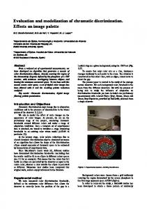
mentioned internal surface. The relations between stresses and displacements at the fictitious surface can be used to derive elements of a matrix, which represents the response of the exterior space in regard to this surface. Between this surface and the top surface, a small FEM domain shall be introduced (figure 1.1). Taking into account the filter characteristics mentioned above, the size of this FEM domain and of the corresponding elements could be chosen in accordance with the necessary error limitations.

top surface

ΩB FEM fictitious surface

Figure 1.1 FEM Mesh

Finally the "structure" and the additional small FEM domain taking account of the derived matrix acting at its exterior surface have to be analyzed. In this approach the soil behavior is included by the additional FEM domain between the soil- "structure"-interface and the fictitious exterior surface where relations are introduced which describe the half-space. A transition to the time domain can be realized by means of an additional FT, which leads to a description by means of a convolution. In the present works, based on Zirwas’ works, will be developed a coupling method, ITM-FEM for 3-D structure

1.3 Subjects Covered The second chapter of this work will cover the background theory of modelling soil as a half-space including layered half-space and solution for volume forces in the half-space in frequency domain. In the third chapter a dynamic matrix for excavated half-space is developed using Integral Transform Method. Here will be introduced a substitute model for soil, substructure and upper structure. The coupling process between ITM and FEM will be described in chapter four, and some test will be done to prove this Coupling Method. In chapter five, a simple practical example will be taken to show the advantage of this method and the results will be shown graphically to easier the interpretation. The summary of this work is written in the last chapter with some conclusion and suggestion.

______________________________________________________________________________________________________

Chapter 2 Modelling of Soil In this chapter the soil will be considered as a semi-infinite medium in z-direction with unbounded domain in x- and y-directions. The material properties are assumed to be isotropic, homogeneous and linear elastic, and the material damping will be independent of frequency. Although the soil is assumed as unbounded homogeneous half-space, the properties are allowed to vary with depth but remain constant within the individual layers. This configuration is called a layered half-space. In the following, the fundamental equations of elastodynamics are summarized.

2.1 Propagation of Waves in Continuum The state of stress in an elemental volume of a loaded body is defined in terms of six components of stress, expressed in a vector form as

{σ }T

[

= σ xx

σ yy σ zz τ xy τ yz τ zx ]

(2.1)

where σ xx , σ yy , and σ zz are the normal components of stress, and τ xy ,τ yz , and τ zx are the components of shear stress. Stresses acting on a positive face of the elemental volume in a positive coordinate direction are positive; those acting on a negative face in a negative direction are positive; all others are negative. A positive face is the one on which normal vector is directed outward from the element points in a positive direction. Corresponding to the six stress components in equation (2.1), the state of strain at a point can be divided into six strain components given by the following strain vector:

{ε }T

[

= ε xx

ε yy ε zz γ xy γ yz γ zx ]

(2.2)

The stress-strain relationship for elastic, isotropic and homogeneous material is given by

σ xx = λ∆ + 2µε xx

τ xy = 2µε xy

σ yy = λ∆ + 2µε yy

τ yz = 2µε yz

σ zz = λ∆ + 2µε zz

τ zx = 2µε zx

(2.3)

with ∆ = ε xx + ε yy + ε zz

4

(2.4)

Propagation of Waves in Continuum

5

_______________________________________________________________________________________________________

and ∂u ∂v ∂w ε yy = ε zz = ∂x ∂y ∂z 1  ∂u ∂v  1  ∂v ∂w  1  ∂w ∂u   γ zx =  =  +  γ yz =  + +  2  ∂y ∂x  2  ∂z ∂y  2  ∂x ∂z 

ε xx =

γ xy

(2.5)

µ and λ are Lame constants and expressed by E 2(1 + υ )

(2.6)

Eυ (1 + υ )(1 − 2υ )

(2.7)

µ =G= λ=

with υ as Poisson ratio and E as Young’s modulus. The equations of motion in terms of stresses in the absence of body forces are given by

∂σ xx ∂τ xy ∂τ xz ∂ 2u + + =ρ 2 ∂x ∂y ∂z ∂t

(2.8a)

∂τ yx ∂σ yy ∂τ yz ∂ 2v + + =ρ 2 ∂x ∂y ∂z ∂t

(2.8b)

∂τ zx ∂τ zy ∂σ zz ∂2w + + =ρ 2 ∂x ∂y ∂z ∂t

(2.8c)

Substitution of equations (2.3), (2.4) and (2.5) into the preceding equations yields

ρ

∂ 2u ∂∆ = (λ + µ ) + µ∇ 2u 2 ∂t ∂x

(2.9a)

ρ

∂ 2v ∂∆ = (λ + µ ) + µ∇ 2 v 2 ∂y ∂t

(2.9b)

ρ

∂2w ∂∆ = (λ + µ ) + µ∇ 2 w 2 ∂z ∂t

(2.9c)

with

∂2 ∂2 ∂2 ∇ = 2+ 2+ 2 ∂x ∂y ∂z 2

(2.10)

Differentiating equations (2.9a), (2.9b), and (2.9c) with respect to x, y, and z, respectively, and adding, ______________________________________________________________________________________________________

6

Modelling of Soil

_______________________________________________________________________________________________________

ρ

 ∂ 2∆ ∂ 2∆ ∂ 2∆   ∂u ∂v ∂w  ∂ 2  ∂u ∂v ∂w   2 + 2 + 2  + µ∇ 2  + ( )    = + λ µ + + + 2   ∂y ∂z  ∂t  ∂x ∂y ∂z   ∂x ∂y ∂z   ∂x

(2.11)

or

∂ 2 ∆ (λ + 2µ ) 2 = ∇ ∆ ρ ∂t 2

(2.12)

This second order partial differential equation is known as longitudinal or dilatational wave or P-wave equation in an unbounded medium and implies that the dilatation is propagated through the medium with velocity:

λ + 2µ ρ

cp =

(2.13)

To obtain the shear wave velocity, we express the rotations as

1  ∂w ∂v  1  ∂u ∂w  1  ∂v ∂u  ω x =  −  ω y =  −  ω z =  −  2  ∂y ∂z  2  ∂z ∂x  2  ∂x ∂y 

(2.14)

and then we take equation (2.9b) and differentiate it with respect to z. After that we take again equation (2.9c) and differentiate it with respect to y, subtracting one from another, we get :

∂ 2ω x µ 2 = ∇ ωx ρ ∂t 2

(2.15a)

Using the process of similar manipulation, one can also obtain two more equations similar to equation (2.15) : ∂ 2ω y

µ 2 ∇ ωy ρ

(2.15b)

∂ 2ω z µ 2 = ∇ ωz ρ ∂t 2

(2.15c)

∂t

2

=

These are the distortional wave or shear wave or S-wave equations where rotations ωx , ωy and ωz propagate with a velocity cs =

µ ρ

(2.16)

______________________________________________________________________________________________________

Damping

7

_______________________________________________________________________________________________________

2.2 Damping Consider a classical analytical model of a linear SDOF system consist of spring-mass-dashpot model. When this system is subjected to harmonic excitation, poeiωt , its equation of motion is mu + cu + ku = p o e iωt

(2.17)

The bar in the equation above shows that u is a complex number. In this text, the bar designates complex number. The complex frequency response H (ω ) is evaluated as

H (ω ) =

1 1 − r + i (2ζr )

(

2

)

(2.18)

k m

(2.19)

with

ωn = ζ =

c cm = ccr 2k

(2.20)

ω ωn

(2.21)

r=

Another way to introduce a damping mechanism is by using complex stiffness muDD + k (1 + iγ )u = p o e iωt

(2.22)

where γ is the structural damping factor. The complex term k (1 + iγ )u represent both the elastic and damping forces at the same time. This complex stiffness k (1 + iγ ) has no physical meaning, however, in the same engineering sense as the elastic stiffness. The complex frequency response H (ω ) for equation (2.22) is

H (ω ) =

1

(1 − r ) + iγ 2

(2.23)

By comparing the denominators of equations (2.23) and (2.18) we see that the factor γ in the former corresponds to the factor (2ζr) in the latter. Since, when damping factors are small (as is generally the case in a structure), damping is primary effective at frequency in the vicinity of resonance, it

______________________________________________________________________________________________________

8

Modelling of Soil

_______________________________________________________________________________________________________

can be seen that, under harmonic excitation condition, structural damping is essentially equivalent to viscous damping with

ζ =

γ γ ≅ 2r 2

(2.24)

5

ζ = 0.

γ=ζ=0

Frequency Response |H|

4

γ = 0.2

3

ζ=

γ = 0.4

2

1

0 0

0,5

1

1,5

2

2,5

3

Fr e q u e n cy Ratio , r

Figure 2.1 Response of system with structural damping factor and viscous damping

From figure 2.1 we can see that the differences between forced vibration with structural damping factor γ and forced vibration with viscous damping ratio ζ are not significant. Therefore it is reasonable to use complex stiffness for damping mechanism. Another way to get the complex stiffness is by simply replacing the real modulus of elasticity E with the complex value of E :

E = E (1 + i 2ζ )

(2.25)

where ζ is damping ratio. This method will be used here.

2.3 Equation of Motion and Wave Equation in Elastic Half-space Equation (2.9a), (2.9b), and (2.9c) represent the equations of motion of an isotropic, homogeneous elastic body in the absence of body forces, in matrix form we can write these equations as ______________________________________________________________________________________________________

Equation of Motion and Wave Equation in Elastic Half Space

9

_______________________________________________________________________________________________________

 2  µ ∇ [I ] + (λ + µ ) ∇ 

∇ −ρ

T

∂2  [I ]{U } = {0} ∂t 2 

(2.26)

with

{U } = [u x

uy

∂ ∇ =  ∂x

∂ ∂y

∇2 = ∇ ⋅ ∇

=

T

]

(2.27)

∂ ∂z 

(2.28)

∂2 ∂2 ∂2 + + ∂x 2 ∂y 2 ∂z 2

(2.29)

uz

T

1 0 0 [I ] = 0 1 0 0 0 1

(2.30)

These Lamé’s equations consist of three coupled partial differential equations, and these equations can be uncoupled using Helmholtz’s potentials

{U } =

∂ Φ + [ X ]{Ψ} T

(2.31)

with

{Ψ} = [Ψx

Ψy

Ψz

]

(2.32)

− ∂∂z

  −  0 

(2.33)

T

and  0 [X ] =  ∂∂z − ∂∂y 

0 ∂ ∂x

∂ ∂y ∂ ∂x

where Φ and Ψ are potential functions. Substituting Eq.(2.31) into Eq.(2.26) gives ∇

T

((λ + 2µ )∇ Φ − ρ ΦCC ) + [X ]{µ∇ {Ψ} − ρ {ΨCC }} = {0} 2

2

(2.34)

This equation will be satisfied if each vector vanishes, thus giving

∇2Φ −

1 Φ=0 2 cp

(2.35)

______________________________________________________________________________________________________

10

Modelling of Soil

_______________________________________________________________________________________________________

∇ 2 {Ψ} −

1 >> {Ψ} = 0 2 cs

(2.36)

These two equations are analogue with the wave equations from (2.12) and (2.15)- (2.17), i.e. Pwave and S-wave equation with velocities cp , equation (2.13) and cs , equation (2.18). If we look at equation (2.31), the four potential fields Φ, Ψx, Ψy and Ψz are not uniquely determined by the three displacement ux , uy and uz . As a special gauge Ψz is set to zero, then equation (2.31) can be written as u x = Φ ,x − Ψy,z u y = Φ , y − Ψx, z

(2.37)

u z = Φ , z − Ψx, y + Ψ y , x

To solve these equations the Integral Transform Method (ITM) using Fourier Transform will be used here and schematically described in figure 2.2.

Fourier Transformation

Lame diff. Eq

Ordinary diff. Eq

Usual FEM or BEM procedure

Response

Analytical Solution

Inverse Fourier Transformation

Transformed response

Figure 2.2 Characteristic of the applied ITM procedure

The Fourier Transform fˆ (k x ) of a function f ( x ) is defined by the integral : +∞ fˆ (k x ) = ∫ f ( x )e −ik x x dx −∞

(2.38)

This formula can be interpreted as linear operator transforming f ( x ) to fˆ (k x ) . In the case of a function with several independent variables, multiple integrals are used, concerning the transformation of each variable. By performing an integral transform (the symbol will be used here for Fourier Transform) on the governing equations and boundary conditions of the problem, we obtain ordinary differential equations instead of partial differential equations; (x,y,z,t) (kx,ky,z,ω) . Thus it is easier to find solutions satisfying the boundary conditions in the transform domain. Afterwards we have to invert the solutions, by inversion formula, in the initial domain, symbolized by . The Inverse Fourier Transform is defined by : ______________________________________________________________________________________________________

Equation of Motion and Wave Equation in Elastic Half Space

11

_______________________________________________________________________________________________________

f (x ) =

1 2π

∫

+∞

−∞

fˆ (k x )e ik x x dk x

(2.39)

By a threefold Fourier transform x kx , y ky and t ω equation (2.35) and equation (2.36) are transformed and one arrives at the transformed domain and now we have ordinary differential equations regarding the z-direction  ω2  ˆ ∂ 2Φ 2 2 ˆ  Φ + − k − k =0 x y 2 c 2  ∂ z p  

(2.40)

ˆ ω2 ∂ 2Ψ 2 2 ˆ i   − k − k Ψ + =0 x y i 2 2 c  z ∂  s 

(2.41)

For the above differential equations, the solutions can be given as ˆ = A1e λ1 z + A2 e − λ1 z Φ

(2.42)

ˆ = B e λ2 z + B e − λ2 z Ψ 1i 2i i

(2.43)

with

λ12 = k x2 + k y2 − k p2

;

λ22 = k x2 + k y2 − k s2

ω cp

;

ks =

kp =

(2.44)

ω cs

(2.45)

Transforming equation (2.37) gives the displacement equations in transformed domain

ˆ ˆ −Ψ uˆ x = ik x Φ y, z ˆ ˆ −Ψ uˆ y = ik y Φ x, z

(2.46)

ˆ + ik Ψ ˆ ˆ , z − ik y Ψ uˆ z = Φ x x y Substituting equations (2.42) and (2.43) into equation (2.46) give uˆ x  ik x uˆ  = ik  y  y uˆ z   λ1

ik x

0

0

− λ2

ik y − λ1

λ2 − ik y

− λ2 − ik y

0 ik x

λ2   0  ⋅ {C } ik x 

(2.47)

with

{C}T

[

= A1e zλ1

A2 e − zλ1

B x1e zλ2

B x 2 e − zλ2

B y1 e z λ 2

B y 2 e − zλ2

]

(2.48)

and the stresses in transformed domain can be written as ______________________________________________________________________________________________________

12

Modelling of Soil

_______________________________________________________________________________________________________

 − 2k x 2 − λµ k p 2  σˆ x    σˆ  2 2 λ  − 2k y − µ k p  y  2k 2 − k 2  σˆ z  r s   = µ ˆ σ k k − 2  x y  xy   σˆ yz  2ik y λ1     2ik x λ1 σˆ zx 

− 2k x − λµ k p

2

0

0

− 2ik x λ2

− 2k y − λµ k p

2

2ik y λ2

− 2ik y λ 2

0

− 2ik y λ 2 ik x λ 2 λ2 2 + k y 2 kxk y

2ik y λ 2 ik x λ2 λ2 2 + k y 2 kxk y

2ik x λ2 − ik y λ2 − kxk y 2 2 − λ2 − k x

2

2

2k r − k s − 2k x k y − 2ik y λ1 − 2ik x λ1 2

2

  0  − 2ik x λ2  {C } ik y λ 2  − kxk y   2 2 − λ2 − k x  (2.49)

2ik x λ2

with kr = k x + k y 2

2

(2.50)

The unknown coefficients A1, A2, B1x, B1y, B2x, and B2y in equation(2.48) can be determined from the boundary conditions in the original domain.

2.4 Layered Half-space This half-space configuration is allowed to have layers, so it is possible to model soil configuration which consist of horizontal layers resting on a half space. The properties vary with depth but remain constant within the individual layers. In a layered half-space, it is better to use constants A1 , B1i instead of A1 , B1i according to

A1e λ1 z = A1e λ1h e − λ1h e λ1z = A1e λ1 ( z −h ) B1i e λ1 z = B1i e λ2 h e −λ2 h e λ2 z = B1i e λ2 ( z − h )

(2.51)

h>z with h is the depth of the layer. The displacement in the transformed domain in Eq.(2.47) can be rewritten as : λ ( z −h ) uˆ x  ik x e 1 uˆ  = ik e λ1 ( z −h )  y  y uˆ z   λ1e λ1 ( z −h )

ik x e −λ1z ik y e −λ1 z − λ1e −λ1 z

− λ 2 e λ2 ( z − h )

0

0

λ2 e λ (z −h ) − ik y e λ ( z −h )

− λ 2 e − λ2 z − ik y e −λ2 z

ik x e

Bx2

By2

2

2

0 λ2 ( z − h )

λ 2 e −λ z   0  ⋅ {C }(2.52) ik x e −λ z  2

2

with

{C } = [A T

1

A2

B x1

B y1

]

(2.53)

With the help from Finite Element Method, embedded structures can be modelled and analysed. Figure 2.3 shows the possibility of structure configuration that can be analysed by this coupling method (ITM-FEM).

______________________________________________________________________________________________________

Layered Half-space

13

_______________________________________________________________________________________________________

h

Figure 2.3 Soil-structure interaction system with layered half-space

______________________________________________________________________________________________________

14

Modelling of Soil

_______________________________________________________________________________________________________

2.5 Forced Vibration of The Layered Half-space We shall now consider a problem of forced vibration of the half-space caused by volume forces. The equation of motion of an isotropic, homogeneous elastic body by the presence of body forces {q}, can be written as

 2  µ ∇ [I ] + (λ + µ ) ∇ 

T

∇ −ρ

∂2  [I ]{U } = −{q} ∂t 2 

(2.54)

with

{q} = [q x

qy

qz

]

T

(2.55)

If we divide the above equation with µ , we get  2 ∇ [I ] + (κ + 1) ∇ 

T

∇ −

1 ∂2  [I ]{U } = {p} 2 2 c s ∂t 

(2.56)

with

{p} = [ p x

κ=

λ µ

py

pz

(2.57)

]

T

=−

1 {q} µ

(2.58)

and cs is the velocity of shear wave from equation (2.16). Equation (2.54) above is an inhomogeneous partial differential equation with inhomogeneous part {p} . Thus, from this equation we have two parts of the solutions; the homogeneous solution, if {p} = {0} and the particular solution if {p} ≠ {0}. Figure 2.4 shows a volume force {q} that has 5 force contributions; {q1 }, {q 2 }, {q3 }, {q 4 } and {q5 } which act on surface Γ1 , Γ2 , Γ3 , Γ4 and Γ5 respectively;

{q} = {q1 } + {q 2 } + {q3 } + {q 4 } + {q5 }

(2.59)

Γ ≡ Γ1 ⊕ Γ2 ⊕ Γ3 ⊕ Γ4 ⊕ Γ5

(2.60)

The forces {q} that act on surface Γ are intended to approximate the stresses on the half-space that are produced by the structures above. The form of Γ as given in figure (2.4) is chosen in order to represent an excavation, but we can also choose another form like open box or other reasonable forms. Fictitious loads are introduced as Fourier series with unknown coefficients (Clmn) ______________________________________________________________________________________________________

Forced Vibration of The Layered Half-space

15

_______________________________________________________________________________________________________

h

bx

bx

h

Γ4

h

y = x - ( by - bx )

y = -x - ( by - bx )

by

Γ2

Γ5

Γ1 X

0

I

by y = -x + ( by - bx )

y = x + ( by - bx )

Γ3

h

II Y

q2 h

q1

0

q5

Z

z = x + ax

ax

X

z = -x + ax X1

01

bx 45°

Z1

Section I q4 h z = y + ay

q3

0

q5

ay

Z 01

Y

z = -y + ay Y1

by 45°

Z1

Section II Figure 2.4 Forces in the layered half-space

Regarding equation (2.59), equation (2.58) can be rewritten as ______________________________________________________________________________________________________

16

Modelling of Soil

_______________________________________________________________________________________________________

{p} = {p1 } + {p 2 } + {p3 } + {p 4 } + {p5 }

(2.61)

with

{p1} = ∑ ∑ δ ( z + x − ax ) ⋅ [H (x + y + (by − bx )) − H (− x + y − (by − bx ) )]⋅ [H ( z ) − H ( z − h)]⋅ e N

M

 πm πn  x+ y  i  ax a y  

n =− N m =− M

{tmn }

(2.62)

{p2 } = ∑ ∑ δ ( z − x − ax ) ⋅ [H (− x + y + (by − bx ) ) − H (x + y − (by − bx ) )]⋅ [H ( z ) − H ( z − h)]⋅ e N

M

 πm πn  i x+ y   ax a y  

n= − N m = − M

{tmn }

(2.63)

{p3 } = ∑ ∑ δ ( z + y − a y ) ⋅ [H (x + y − (b y − bx ) ) − H (x − y + (b y − bx ) )]⋅ [H ( z ) − H ( z − h)]⋅ e N

M

 πm πn  i x+ y   ax a y  

n=− N m=− M

{t mn }

(2.64)

{p4 } = ∑ ∑ δ ( z − y − a y ) ⋅ [H (x − y − (by − bx ) ) − H (x + y + (by − bx ))]⋅ [H ( z ) − H ( z − h)]⋅ e N

M

 πm πn  x+ y  i  ax a y  

n =− N m= − M

{tmn }

(2.65)

{p5 } = ∑ ∑ δ ( z − h) ⋅ [H ( x + bx ) − H ( x − bx )]⋅ [H ( y + by ) − H ( y − by )]⋅ e N

M

n =− N m =− M

{t mn } = [t xmn

t ymn

t zmn

]

T

 πm πn  x+ y  i  ax a y  

{tmn }

(2.66) (2.67)

and H is Heaviside distribution.

2.5.1 Particular Solution for Upper Layer Transforming the forces in equation (2.61) and the equation of motion in (2.56) regarding the two coordinates x, y kx , ky and time t ω , and extending the load {p1 }, {p 2 }, {p3 }, {p 4 } and

{p5 } over the whole domain − ∞ ≤ z ≤ +∞

, gives

{p( x, y, z )}

{pˆ (k , k x

y

, z )}

Using Maple® Package Program, one can obtain the load in transfomed domain, and can be written as :

______________________________________________________________________________________________________

Particular Solution for Upper Layer

17

_______________________________________________________________________________________________________

{pˆ } = ∑ ∑ [A e N

j

M

n=− N m =− M

=

( κ1 j z +κ 2 j ) i

j

− Aj e

( κ 3 j z +κ 4 j ) i

]{t

mn

}

j = 1,2 ,3,4

(2.68)

δ ( z − h ) −iα b −iα b iα b {t mn } e − e iα b e −e n = − N m = − M α 1α 2 N

[

M

∑ ∑

1 x

1 x

][

2 y

2 y

]

j=5

with

A = [ A1 + (α 1 + α 2 ) − (α + α ) [κ ] =  1 2 + (α 2 + α 1 )  − (α 2 + α 1 )

A2

A3

[

A4 ] = iα 2−1

− α 2 ∆b − (α 1 + α 2 )a x + α 2 ∆b + (α 1 + α 2 )a x + α 1 ∆b − (α 2 + α 1 )a y − α 1∆b + (α 2 + α 1 )a y

α1 = k x −

]

(2.69)

+ α 2 ∆b − (α 1 − α 2 )a x  − α 2 ∆b + (α 1 − α 2 )a x  − α 1 ∆b − (α 2 − α 1 )a y   + α 1 ∆b + (α 2 − α 1 )a y 

(2.70)

− iα 2−1 iα 1−1 + (α 1 − α 2 ) − (α 1 − α 2 ) + (α 2 − α 1 ) − (α 2 − α 1 )

− iα 1−1

πn πm α2 = ky − ax ay

(2.71)

∆b = b y − bx

(2.72)

The transformed equation of motions one has :

uˆ x   pˆ x       ∂ ∂2 [d1 ] + [d 2 ] + 2 [d 3 ] uˆ y  =  pˆ y  ∂z ∂z   uˆ   pˆ   z  z

(2.73)

with − 2k x2 − κk x2 − k y2 + k s2 [d1 ] =  − (1 + κ )k x k y  0 

− (1 + κ )k x k y − 2k y2 − κk y2 − k x2 + k s2 0

  0  − k x2 + k y2 − k s2  0

(

)

(2.74)

 0 0 ik x (1 + κ )    0 ik y (1 + κ ) [d 2 ] =  0 ik x (1 + κ ) ik y (1 + κ )  0  

(2.75)

0  1 0  [d3 ] = 0 1 0  0 0 2 + κ 

(2.76)

______________________________________________________________________________________________________

18

Modelling of Soil

_______________________________________________________________________________________________________

For the particular solution of equation (2.56) we use the same exponential function as for the loading:

{uˆ }= ∑ ∑ ∑ ({U }A ⋅ e 4

N

M

p

1j

j =1 n = − N m = − M

(κ 1 j z +κ 2 j ) i

j

− {U 2 j }A j ⋅ e

)

(κ 3 j z +κ 4 j ) i

(2.77)

with

{U } = [U

1 xj

U 1 yj

U 1zj

{U } = [U

2 xj

U 2 yj

U 2 zj

T

1j

T

2j

]

(2.78)

]

(2.79)

Substituting Eq.(2.77) into Eq.(2.73) gives

[ D1 j ] [0]  {U1 j } {t mn }   [0] [ D ] {U } =  2j   2j  {t mn } 

(2.80)

with

(

)

 − λ22 + κ 12j − (1 + κ )k x2  [ D1 j ] =  − (1 + κ )k x k y  − (1 + κ )k xκ 1 j 

(

)

 − λ22 + κ 32j − (1 + κ )k x2  [ D2 j ] =  − (1 + κ )k x k y  − (1 + κ )k xκ 3 j 

− (1 + κ )k x k y

(

− (1 + κ )k xκ 1 j

)

− λ + κ − (1 + κ )k − (1 + κ )k yκ 1 j 2 2

2 1j

2 y

− (1 + κ )k x k y

(

  − (1 + κ )k yκ 1 j  (2.81) − λ22 + κ 12j − (1 + κ )κ 12j 

(

)

− (1 + κ )k xκ 3 j

)

− λ22 + κ 32 j − (1 + κ )k y2 − (1 + κ )k yκ 3 j

  − (1 + κ )k yκ 3 j  (2.82) 2 2 2  − λ2 + κ 1 j − (1 + κ )κ 3 j 

(

)

)

− (1 + κ )k xκ 1 j − (1 + κ )k yκ 1 j

To get {U1j} & {U2j} we have to invert [D1j] and [D2j]

[D ]

−1

1j

(

)

(

 λ22 + κ 12j + (1 + κ ) κ 12j + k y2 1  = − (1 + κ )k x k y det 1 j   − (1 + κ )k x K1 j 

)

− (1 + κ ) k x k y λ + κ + (1 + κ ) κ 12j + k x2

(

2 2

2 1j

)

(

− (1 + κ )k yκ 1 j

(λ

2 2

+ κ 12j

)

   + (1 + κ ) k x2 + k y2 

(

)

(2.83)

[D ]

−1

2j

1 = det 2 j

(

)

(

 λ22 + κ 32 j + (1 + κ ) κ 32 j + k y2  − (1 + κ )k x k y   − (1 + κ ) k x K 3 j 

)

− (1 + κ )k x k y λ + κ + (1 + κ ) κ 32j + k x2

(

2 2

2 3j

)

(

− (1 + κ )k yκ 3 j

)

(λ

− (1 + κ )k xκ 3 j − (1 + κ )k yκ 3 j 2 2

+ κ 32 j

)

   + (1 + κ ) k x2 + k y2 

(

)

(2.84) with

______________________________________________________________________________________________________

Particular Solution for Upper Layer

19

_______________________________________________________________________________________________________

det1 j =

det 2 j =

(

)

(

)

(

)

− (1 + κ )k s2 λ22 + κ 12j − (2 + κ ) λ22 + κ 12j 2

(λ

2 2

(

+ κ 12j

)

)

3

− (1 + κ )k s2 λ22 + κ 32j − (2 + κ ) λ22 + κ 32 j 2

(λ

2 2

+ κ 32 j

)

(2.85) 3

(2.86)

{U } = [D ] {t }

(2.87)

{U } = [D ] {t }

(2.88)

−1

1j

1j

mn

−1

2j

2j

mn

Substituting equations (2.87) and (2.88) into equation (2.77) gives the particular solution of equation (2.73).

2.5.2 Homogeneous Solution

{ } { }

The homogeneous solutions for a system shown in figure 2.3 consist of two parts ; uˆ h & uˆ1h , the first is for the upper layer and the second is for the half-space. We will base our homogeneous solution on equation (2.46) and must satisfy these 9 boundary conditions below

τˆ xzp ( z = 0) + τˆ xzh ( z = 0) = 0 τˆ yzp ( z = 0) + τˆ yzh ( z = 0) = 0 σˆ zzp ( z = 0) + σˆ zzh ( z = 0) = 0 τˆ xzp ( z = h) + τˆxzh ( z = h) − τˆxh z ( z1 = 0) = qˆ 5 x τˆ yzp ( z = h) + τˆ yzh ( z = h) − τˆ yh z ( z1 = 0) = qˆ 5 y σˆ zzp ( z = h) + σˆ zzh ( z = h) − σˆ zh z ( z1 = 0) = qˆ 5 z 1 1

(2.89)

1 1

1 1

uˆ ( z = h) + uˆ ( z = h) − uˆ ( z1 = 0) = 0 uˆ ( z = h) + uˆ ( z = h) − uˆ ( z1 = 0) = 0 uˆ ( z = h) + uˆ ( z = h) − uˆ ( z1 = 0) = 0 p x p y p z

h x1 h y1 h z1

h x h y h z

On the upper layer z=0, regarding equations (2.49) and (2.51), we can write the stress equations in transformed domain as

{σˆ } h

z =0

= [A1 ]{C1 }

(2.90)

with

{σˆ }

h T z =0

[

= τˆxzh ( z = 0) τˆ yzh ( z = 0) σˆ zzh ( z = 0)

{C } = [A T

1

11

A21

B x11

B x 21

B y11

B y 21

]

(2.91)

]

(2.92)

______________________________________________________________________________________________________

20

Modelling of Soil

_______________________________________________________________________________________________________

 2ik x λ11e −λ11h [A1 ] = µ1  2ik y λ11e −λ11h  2k r2 − k s2 e −λ11h 

(

− 2ik x λ11 − 2ik y λ11 2k r2 − k s2

)

k x k y e −λ21h λ221 + k y2 e −λ21h − 2ik y λ 21e −λ21h

(

)

kxky 2 λ21 + k y2 2ik y λ 21

− (λ221 + k x2 )e −λ21h − k x k y e −λ21h 2ik x λ21e −λ21h

− (λ221 + k x2 )   − kxky  − 2ik x λ21 

(2.93)

λ12i = k x2 + k y2 − k pi2

(2.94)

λ22i = k x2 + k y2 − k si2

(2.95)

{σˆ }

(2.96)

And for the particular solution p

z =0

= [G ]{S }z =0

with

{σˆ }

p T z =0

[

= τˆxzp ( z = 0) τˆyzp ( z = 0) σˆ zzp ( z = 0)

 0 [G ] =  0 i λ k x 

{S }Tz =o = [uˆ xp ( z = 0)

]

(2.97)

µik x µ 0 0   µik y 0 µ 0  0 0 0 λ + 2 µ 

0 0 iλ k y

(2.98)

uˆ yp ( z = 0) uˆ zp ( z = 0) uˆ xp, z ( z = 0) uˆ yp, z ( z = 0) uˆ zp, z ( z = 0)

]

(2.99)

The vector {S }z =o has to be calculated from equations (2.77), (2.87), (2.88) and as we see from these three equations, {S }z =o is dependent from {t mn } On the boundary z = h and z1=0 , the displacement and the stresses in transformed domain are: Upper Layer, z = h

{uˆ } h

z =h

= [A2 ]{C1 }

(2.100)

with

{uˆ }

h T z =h

ik x [A2 ] = µ1 ik y  λ11 

[

= uˆ xzh ( z = h) uˆ hyz ( z = h) uˆ zzh ( z = h) ik x e −λ11h

0

0

ik y e −λ11h

λ 21 − ik y

− λ 21e −λ21h

− λ11e

− λ11h

− ik y e

− λ 21 −λ21h

0 ik x

]

(2.101)

λ 21e −λ 0 ik x e −λ

   21h   21h

(2.102)

and the stresses, regarding equations (2.49) and (2.51)

______________________________________________________________________________________________________

Homogeneous Solution

21

_______________________________________________________________________________________________________

{σˆ } h

= [A3 ]{C1}

z =h

(2.103)

with

{σˆ }

h T z =h

 2ik x λ11 [A3 ] = µ1  2ik y λ11 2k r2 − k s2 

[

= τˆxzh ( z = h) τˆyzh ( z = h) σˆ zzh ( z = h)

− 2ik x λ11e −λ11h − 2ik y λ11e −λ11h

(2k

2 r

)

−k e 2 s

−λ1h

k x k y e −λ21h λ221 + k y2 e −λ21h

kxky 2 λ21 + k y2

(

− 2ik y λ21

)

2ik y λ21e −λ21h

]

(2.104)

− (λ221 + k x2 ) − (λ221 + k x2 )e −λ21h   − kxk y − k x k y e −λ21h  − 2ik x λ21e −λ21h  2ik x λ 21

(2.105) And for the particular solution, {σˆ p }z =h ; the stresses at z=h, can be calculated analogue with equations (2.96)-(2.99). Lower Layer / Half-space, z1=0

{uˆ }

h 1 z1 = 0

= [ A4 ]{C 2 }

(2.106)

with

{uˆ }

h T 1 z1 = 0

[

= uˆ xh1z1 ( z1 = 0) uˆ hy1 z1 ( z1 = 0) uˆ zh1 z1 ( z1 = 0)

{C } = [A T

2

22

Bx 22

(2.107)

]

(2.108)

λ2   0 ik x 

(2.109)

By 22

 ik x [A4 ] =  ik y − λ1 

− λ2 − ik y

{σˆ }

= [ A5 ]{C2 }

0

]

and the stresses h 1 z1 = o

(2.110)

with

{σˆ }

h T 1 z1 = 0

[

= τˆxh1 z1 ( z1 = 0) τˆ yh1 z1 ( z1 = 0) σˆ zh1 z1 ( z1 = 0)

 − 2ik x λ1 [A5 ] = µ 2  − 2ik y λ1 2k r2 − k s2 

kxk y

λ22 + k y2 2ik y λ 2

− (λ22 + k x2 )  − kxk y  − 2ik x λ 2 

]

(2.111)

(2.112)

______________________________________________________________________________________________________

Homogeneous Solution

22

_______________________________________________________________________________________________________

Regarding equations Substituting equations (2.90) - (2.112), boundary conditions in equation (2.89) can be rewritten as

[A]{C } = { S BC ({tmn }) }

(2.113)

 [ A1 [A] = [ A3 [ A2

] [ 0 ] ] [A5 ] ] [A4 ]

(2.114)

{C } = [{C } {C } ]

(2.115)

with

T

T

T

1

2

{

}

 − σˆ p ({t mn }) z =0 { S BC ({t mn }) } = { qˆ 5 ({t mn }) } − σˆ p ({t mn })  uˆ p ({t mn }) z = h 

{

{

}

  z =h   

}

(2.116)

By inverting [A] , we can get {C } from

{C } = [A] { S ({t }) } −1

BC

mn

(2.117)

______________________________________________________________________________________________________

Examples for Forced Vibration of The Layered Half-space

23

_______________________________________________________________________________________________________

2.6 Examples for Forced Vibration of The Layered Halfspace 2.6.1 Special Cases, h = 0 If the depth where the forces act, h in figure 2.4 is equal to zero, h = 0, means that the forces act on the surface of half-space. The particular solutions disappear and we have only homogeneous solutions for this problem. The boundary conditions from equation (2.89) become:

σˆ xh z ( z1 = 0) = −qˆ 5 x σˆ yh z ( z1 = 0) = −qˆ 5 y σˆ zh z ( z1 = 0) = −qˆ 5 z 1 1

(2.118)

1 1

1 1

Substitution of these equations into equation (2.110) gives :  − 2ik x λ1  qˆ 5 x     − {qˆ5 } = −  qˆ 5 y  = [ A5 ]{C 2 } = µ 2  − 2ik y λ1  2k r2 − k s2  qˆ5 z  

kxk y

λ22 + k y2 2ik y λ2

− (λ22 + k x2 )  A22    − k x k y   Bx 22  − 2ik x λ2   B y 22 

(2.119)

and  A22  {C 2 } =  Bx 22  = −[A5 ]−1 {qˆ 5 }  B y 22   

(2.120)

Substitution of {C 2 }into equation (2.47) gives :

uˆ x  uˆ  = Fˆ ⋅ {qˆ } 5  y uˆ z 

[]

(2.121)

with  ik x e −λ1 z1  Fˆ = −  ik y e −λ1 z1  − λ1e −λ1 z1 

[]

0

λ2 e −λ z 0 ik x e −λ z

  −1  ⋅ [ A5 ] 2 1  

2 1

− λ2 z1

− λ2 e − ik y e −λ2 z1

(2.122)

______________________________________________________________________________________________________

24

Modelling of Soil

_______________________________________________________________________________________________________

[A5 ]−1 = −

1 µ 2 ∆ A5

  − 2ik x λ 2  2 2  k x k y 4λ1λ 2 − 2k r − k s  λ22  2 2 2 2 2  4k y λ1λ 2 − 2k r − k s λ 2 + k y  λ22 

(

− 2ik y λ 2

)

(

)(

−

)

(

)(

4k x2 λ1λ 2 − 2k r2 − k s2 λ22 + k x2 λ22 k x k y 4λ1λ 2 − 2k r2 − k s2 − λ22

(

)

)

∆ A5 = −(2k r2 − k s2 ) + 4k r2 λ1λ 2

 2k − k    − 2ik y λ1    − 2ik x λ1   (2.123) 2 r

2 s

(2.124)

It can be seen from equations (2.123)-(2.124) that for given k x , k y , and z, the displacements in the transformed domain uˆ x , uˆ y , and uˆ z are in functions of forces in transformed domain pˆ 5 x , pˆ 5 y , and pˆ and the matrix [ Fˆ ] is constant and behaves as “flexibility matrix” in transformed domain. 5z

It means that for given k x , k y & z , we only have to calculate [ Fˆ ] once, and then we can obtain any response uˆ , uˆ & uˆ due to the loading pˆ , pˆ & pˆ by simply multiplying {pˆ } by [ Fˆ ]. x

y

z

5x

5y

5z

5

{ }

Analogue for stresses, matrix [ Fˆσ ] can be obtained by substituting Cˆ 2 into equation (2.49), gives :

{σˆ } = [Fˆ ]⋅ {qˆ } h

σ

(2.125)

5

with

{σ } = [σˆ h

( (

σˆ yh

h x1

1

) )

 − 2k x 2 − λµ k p 2 e −λ1z1  2 2 −λ1z1 λ  − 2k y − µ k p e  2k 2 − k 2 e −λ1z1 r s Fˆσ = − µ 2  − 2k x k y e −λ1z1   − 2ik λ e −λ1z1 y 1   − 2ik x λ1e −λ1z1

[ ]

(

)

σˆ zh

1

σˆ xh y

1 1

σˆ yh z

0 − 2ik y λ2e −λ2 z1 2ik y λ2 e −λ2 z1 ik x λ2e −λ2 z1 λ2 2 + k y 2 e −λ2 z1 k x k y e −λ2 z1

(

)

σˆ zh x

1 1

1 1

]

T

(2.126)

   − 2ik x λ2e −λ2 z1  −1  ⋅ [ A5 ] −λ2 z1 ik y λ2e  −λ2 z1  − kxk ye  2 2 − λ2 + k x e −λ2 z1  2ik x λ2 e −λ2 z1 0

(

(2.127)

)

These [ Fˆ ] and [ Fˆσ ] matrices are helpful to calculate the stiffness matrix if the load {q5 } acts on the surface. By using these matrices we can avoid inverting matrix [ A] 9 x 9 in equation 2.114 for every loading {q5 } and every depth, z1. Instead, we just have to invert matrix [ A5 ] 3 x 3 once, and then using this [A5]-1 to get [ Fˆ ] and [ Fˆ ] for every different z1. σ

This is also the reason why computing half-space problem with layer takes much more computingtime rather than half-space without layer. For n additional layers we will have 6n additional interface conditions.

______________________________________________________________________________________________________


25

_______________________________________________________________________________________________________

To illustrate the mechanism of this “flexibility matrix” some examples with single load and block load will be taken and shown in figure 2.5 – 2.11. Figure 2.6 shows the imaginary and real parts of vertical displacement of a single vertical unit load, P= 1 with different frequencies. What we see here actually is an element of the “flexibility matrix” i.e. Fˆ33 . It is clear from figure 2.6, that if we scale the frequency with factor c, it will also scale the wave number ks with factor c, because as we see from equation (2.45 ), ks has a linear function of ω : ks =

ω cs

(2.45)

Figure 2.7 shows vertical unit load spectrum in transformed domain. The total load is the same (10000 kg) but the width (b) of the block force is varied. The equation of a block load in transformed domain (kx , ky) from equation 2.68 can be written as qˆ =

4 sin(bk x ) sin(bk y )

(2.125)

kxk y

It can be seen from equation above that the change of b has influence in the wave number of the load spectrum.

b b

Ptotal = 1 x

y Figure 2.5 Unit block load

Figure 2.8 shows vertical displacements of a single load (with total load = 10000 N) in transformed domain; uˆ z (k x , k y ) . As we notice this spectrum for z = 0, actually it is a multiplication : (vertical displacement spectrum of a single unit load in figure 2.6 for ω=50 rad/s) x ( load spectrum in figure 2.7 for b = 0 ) x 10000 N. For another loading configuration, b=10, as shown in figure 2.10, the displacements for z = 0 can be obtained by multiplyng (figure 2.6 for ω=50 rad/s) x (figure 2.7 for b=10m) x 10000 N.

______________________________________________________________________________________________________

26

Modelling of Soil

_______________________________________________________________________________________________________

As we notice the unit vertical displacement spectrums, uˆ z in figure 2.8, for z=0 in the area between the peaks (the peak of the spectrum is near to k x ≈ − k s and + k s , with ks=0.49), the real part the values is almost zero and outside the peaks area are non zero postive. But for imaginary part, the value between the peaks are non zero negative and the rest is almost zero. Because the most influence areas in this two spectrums (real and imaginary parts) have different sign, it can be understood, why the back transform of these spectrum have also an opposite sign shape. In figure 2.9, we can see, that the peak of the real part of uˆ z has positive sign, but the peak of imaginary part has negative sign. And based on this matter, it can also be understand, that if the changes of the displacement spectrum’s shapes happen at the non zero zone, they can strongly influence the back transform of these spectrum. From figure 2.7, we compare the load spectrum for b = 0 and b = 10 , at the peak area − k s < k x < + k s , they still have the same sign, and they begin to have different sign outside the peak area. Now, if we analize the displacement spectrums for b=10 and z=0 in figure 2.10, for the real part, the most influence area of the spectrum is outside the peak, and a significant change of this area, from positive (figure 2.8, real part, b=0, z=0) to mostly negative (figure 2.10, real part, b=10, z=0) do change the result of the back transform, from positif sign (figure 2.9, real part, b=0, z=0) to negative sign (figure 2.11, real part, b=10, z=0). The imaginary part (figure 2.10, b=10, z=0) has no sign changes at its influence area (compare to figure 2.8, imaginary part, b=0, z=0), that is why the shape of the back transform does not have sign changes (figure 2.9, imaginary part, , b=0, z=0 compare to figure 2.11 ). The peak still has negative sign.

______________________________________________________________________________________________________


27

_______________________________________________________________________________________________________

Vertical Displacement Spectrum Re(U z ') P tot = 1 , h = 0 , z = 0 , ρ = 2000 , ν = 0.2 , ξ = 2% , E = 5.10 7 5,00E-07

4,00E-07

3,00E-07

Re(Uz')

2,00E-07

1,00E-07

0,00E+00

-1,00E-07

-2,00E-07

-3,00E-07

-4,00E-07

-4

-3,5

-3

-2,5

-2

-1,5

-1

-0,5

0

0,5

1

1,5

2

2,5

3

3,5

4

3,5

4

k x at k y = 0

ω = 50

ω = 100

ω = 200

ω = 300

Vertical Displacement Spectrum Im(U z ') P tot = 1 , h = 0 , z = 0 , ρ = 2000 , ν = 0.2 , ξ = 2% , E = 5.10 7

1,00E-07 0,00E+00 -1,00E-07 -2,00E-07

Im(Uz')

-3,00E-07 -4,00E-07 -5,00E-07 -6,00E-07 -7,00E-07 -8,00E-07 -9,00E-07 -1,00E-06 -4

-3,5

-3

-2,5

-2

-1,5

-1

-0,5

0

0,5

1

1,5

2

2,5

3

k x at k y = 0

ω = 50

ω = 100

ω = 200

ω = 300

Figure 2.6 Vertical displacements in transformed domain from a single unit load

______________________________________________________________________________________________________

28

Modelling of Soil

_______________________________________________________________________________________________________

P

Load Spectrum, P tot =1 1,1 1 0,9 0,8 0,7 0,6 0,5 0,4 0,3 0,2 0,1 0 -0,1 -0,2 -0,3 -4

-3,5

-3

-2,5

-2

-1,5

-1

-0,5

0

0,5

1

1,5

2

2,5

3

3,5

4

k x at k y = 0

b=0

b=1

b=2

b=3

b=4

b=5

b=6

P


-3,5

-3

-2,5

-2

-1,5

-1

-0,5

0

0,5

1

1,5

2

2,5

3

3,5

4

k x at k y = 0

b=7

b=8

b=9

b = 10

b = 11

b = 12

b = 13

Figure 2.7 Load spectrums in transformed domain

______________________________________________________________________________________________________


29

_______________________________________________________________________________________________________

Vertical Displacement Spectrum Re(U' z ) P = 10000 , h = 0 , ω = 50 , ρ = 2000 , ν = 0.2 , ξ = 2% , E = 5.10

7

7,00E-03 6,00E-03

P

5,00E-03 4,00E-03 3,00E-03

Re(U' z )

2,00E-03

z

1,00E-03 0,00E+00 -1

-0,5

0

0,5

1

-1,00E-03 -2,00E-03 -3,00E-03 -4,00E-03 -5,00E-03 -6,00E-03 -7,00E-03

kx at ky = 0 z=0

z=1

z=2

z=5

z = 10

Vertical Displacement Spectrum Im(U' z ) P = 10000 , h = 0 , ω = 50 , ρ = 2000 , ν = 0.2 , ξ = 2% , E = 5.10

5,00E-03

7

P

4,00E-03 3,00E-03 2,00E-03

z

1,00E-03 0,00E+00

Im(U' z )

-1,00E-03 -2,00E-03 -3,00E-03 -4,00E-03 -5,00E-03 -6,00E-03 -7,00E-03 -8,00E-03 -9,00E-03 -1,00E-02 -1

-0,5

0

0,5

1

kx at ky = 0 z=0

z=1

z=2

z=5

z = 10

Figure 2.8 Vertical displacement of a single load in transformed domain

______________________________________________________________________________________________________

30

Modelling of Soil

_______________________________________________________________________________________________________

Vertical Displacement Re(U z ) P = 10000 , h = 0 , ω = 50 , ρ = 2000 , ν = 0.2 , ξ = 2% , E = 5.10

7

X at Y = 0 - 30

- 20

- 10

0

9,00E- 05

10

20

30

P

8,00E- 05 7,00E- 05

z

6,00E- 05 5,00E- 05

Re(Uz )

4,00E- 05 3,00E- 05 2,00E- 05 1,00E- 05 0,00E+00 - 1,00E- 05 - 2,00E- 05 - 3,00E- 05

z= 0

z= 1

z= 2

z= 5

z = 10

Vertical Displacement Im(U z ) P = 10000 , h = 0 , ω = 50 , ρ = 2000 , ν = 0.2 , ξ = 2% , E = 5.10

7

X at Y = 0 -30

-20

-10

0

10

20

30

6,00E-05

P

5,00E-05 4,00E-05 3,00E-05

z

2,00E-05

Im(Uz )

1,00E-05 0,00E+00 -1,00E-05 -2,00E-05 -3,00E-05 -4,00E-05 -5,00E-05 -6,00E-05

z=0

z=1

z=2

z=5

z = 10

Figure 2.9 Vertical displacement of a single load in original domain

______________________________________________________________________________________________________


31

_______________________________________________________________________________________________________

Vertical Displacement Spectrum Re(U' z ) P

t ot

= 10000 , h = 0 , b = 10 , ω = 50 , ρ = 2000 , ν = 0.2 , ξ = 2% , E = 5.10

7

6,00E-04

b

p

4,00E-04

z

Re(U' z )

2,00E-04

0,00E+00 -1

-0,5

0

0,5

1

-2,00E-04

-4,00E-04

-6,00E-04

-8,00E-04

kx at ky = 0 z=0

z=1

z=2

z=5

z = 10

Vertical Displacement Spectrum Im(U' z ) P

t ot

= 10000 , h = 0 , b = 10 , ω = 50 , ρ = 2000 , ν = 0.2 , ξ = 2% , E = 5.10

7

kx at ky = 0 -1

-0,5

0

0,5

1

b

1,00E-03

p z

5,00E-04

Im(U' z )

0,00E+00

-5,00E-04

-1,00E-03

-1,50E-03 z=0

z=1

z=2

z=5

z = 10

Figure 2.10 Vertical displacement of a block load in transformed domain

______________________________________________________________________________________________________

32

Modelling of Soil

_______________________________________________________________________________________________________

Vertical Displacement Re(U z ) P

t ot

= 10000 , h = 0 , b = 10 , ω = 50 , ρ = 2000 , ν = 0.2 , ξ = 2% , E = 5.10

7

X at Y = 0 - 30

- 20

-10

0 b

2,00E-06

10

20

30

p z

0,00E+00

Re(Uz )

- 2,00E-06

- 4,00E-06

- 6,00E-06

- 8,00E-06

- 1,00E-05

z= 0

z= 1

z= 2

z= 5

z = 10

Vertical Displacement Im(U z ) P

t ot

= 10000 , h = 0 , b = 10 , ω = 50 , ρ = 2000 , ν = 0.2 , ξ = 2% , E = 5.10

7

b

8,00E-06

p

6,00E-06 z

4,00E-06 2,00E-06

Im(Uz )

0,00E+00 -2,00E-06 -4,00E-06 -6,00E-06 -8,00E-06 -1,00E-05 -1,20E-05 -1,40E-05 -30

-20

-10

0

10

20

30

X at Y = 0 z=0

z=1

z=2

z=5

z = 10

Figure 2.11 Vertical displacement of a block load in original domain

______________________________________________________________________________________________________

Examples for Volume Forces in The Half-space

33

_______________________________________________________________________________________________________

2.6.2 Examples for Volume Forces in The Half-space Figure 2.13 shows the vertical displacement in transformed domain of real and imaginary parts caused by internal load as indicated in the figures, and figure 2.14 shows the vertical displacement in original domain also from real and imaginary parts. These displacements are the results of a loading condition with bx=0, h = 5m (see figure 2.4) with total load 10000 kg. Density ρ is taken 2000 kg/m³, Poisson ratio, ν = 0.2, modulus elasticity, E = 5. 107 N/m² and damping ratio ξ = 2 %. As comparison, another loading condition with the same total load and parameters but different bx=5m is shown in figure (2.15) and (2.16). It can be seen that the maximum displacement in the second loading condition is smaller than the first one, because in the second condition, the loading area is 4 times larger, so the unit load is 4 times smaller than the first. It is interesting to compare the spectrums in figure 2.13 with spectrums in figure 2.15. If we see the peak of the spectrums they have different sign. The peaks in figure 2.12 have negative signs but the peaks in figure 2.14 have positive sign. This phenomenon can be explained if we take a look at figure 2.12. This figure shows load spectrums in transformed domain for b = 14 ~ 20. For b = 20 at kx = ks = 0,49, we have a negative value, but from figure 2.7 for b = 10 at kx = ks = 0,49 we have a positive value.

P


-3,5

-3

-2,5

-2

-1,5

-1

-0,5

0

0,5

1

1,5

2

2,5

3

3,5

4

k x at k y = 0

b = 14

b = 15

b = 16

b = 17

b = 18

b = 19

b = 20

Figure 2.12 Load spectrums in transformed domain

______________________________________________________________________________________________________

34

Modelling of Soil

_______________________________________________________________________________________________________

As can we see from equations (2.116) and (2.117), the displacement responses of loads in the halfspace are also as a function of load spectrum. Although the relationship is not so simple as load on the surface of half-space (equation (2.122)), but it is clear that they depend to the load spectrums too. The loads in figure 2.13 and 2.14 have a total width of 10 m, and the loads in figure 2.15 and 2.16 have a total width of 20 m. If we want to compare the displacement, intuitively we should consider a load spectrum with b=10 m (figure 2.7) for the load with a total width 10 m, and a load spectrum with b=20 m (figure 2.12) for the load with a total width 20 m.

______________________________________________________________________________________________________


35

_______________________________________________________________________________________________________

Vertical Displacement Spectrum Re(U' z ) P tot = 10000 , h = 5 , b = 0 , ω = 50 , ρ = 2000 , ν = 0.2 , ξ = 2% , E = 5.10 7 k x at k y = 0 -1

-0,8

-0,6

-0,4

-0,2

0

8,00E-04

0,2

0,4

p

0,6

0,8

1

h

6,00E-04

4,00E-04

2h

Re(U'z )

2,00E-04

0,00E+00

-2,00E-04

-4,00E-04

-6,00E-04

-8,00E-04

z= 0

z = 2,5

z= 5

z=6

z= 7

z = 10

z = 15

Vertical Displacement Spectrum Im(U' z ) P tot = 10000 , h = 5 , b = 0 , ω = 50 , ρ = 2000 , ν = 0.2 , ξ = 2% , E = 5.10 7 k x at k y = 0 -1

-0,5

p

0

0,5

1

1,00E-03

h 8,00E-04 6,00E-04

2h

4,00E-04

Im(U'z )

2,00E-04 0,00E+00 -2,00E-04 -4,00E-04 -6,00E-04 -8,00E-04 -1,00E-03 -1,20E-03

z=0

z = 2,5

z= 5

z=6

z=7

z = 10

z = 15

Figure 2.13 Vertical displacement in transformed domain

______________________________________________________________________________________________________

36

Modelling of Soil

_______________________________________________________________________________________________________

Vertical Displacement Re(U z ) P tot = 10000 , h = 5 , b = 0 , ω = 50 , ρ = 2000 , ν = 0.2 , ξ = 2% , E = 5.10 7

X at Y = 0 -30

-25

-20

-15

-10

-5

0

5

6,00E-06

10

15

20

25

30

p

4,00E-06

h

2h

2,00E-06

Re(U z)

0,00E+00

-2,00E-06

-4,00E-06

-6,00E-06

-8,00E-06

-1,00E-05

z=0

z = 2,5

z=5

z= 6

z= 7

z = 10

z = 15

Vertical Displacement Im(U z ) P tot = 10000 , h = 5 , b = 0 , ω = 50 , ρ = 2000 , ν = 0.2 , ξ = 2% , E = 5.10 7

X at Y = 0 -30

-25

-20

-15

-10

-5

0

8,00E-06

5

10

15

20

25

30

p

6,00E-06

h

4,00E-06 2h

2,00E-06

Im(Uz )

0,00E+00

-2,00E-06

-4,00E-06

-6,00E-06

-8,00E-06

-1,00E-05

z=0

z = 2,5

z=5

z= 6

z=7

z = 10

z = 15

Figure 2.14 Vertical displacement in original domain

______________________________________________________________________________________________________


37

_______________________________________________________________________________________________________

Vertical Displacement Spectrum Re(U' z ) P tot = 10000 , h = 5 , b = 10 , ω = 50 , ρ = 2000 , ν = 0.2 , ξ = 2% , E = 5.10 7 k x at k y = 0 -1

-0,8

-0,6

-0,4

-0,2

0

0,2

7,50E-04

0,4

0,6

z = 10

z = 15

0,8

1

p

h 5,00E-04

b

h

h

Re(U'z)

2,50E-04

0,00E+00

-2,50E-04

-5,00E-04

z=0

z = 2,5

z=5

z=6

z= 7

Vertical Displacement Spectrum Im(U' z ) P tot = 10000 , h = 5 , b = 10 , ω = 50 , ρ = 2000 , ν = 0.2 , ξ = 2% , E = 5.10 7 k x at k y = 0 -1

-0,5

0

0,5

1,20E-03

1

p

1,00E-03

h

8,00E-04

h

h

b

Im(U'z)

6,00E-04

4,00E-04

2,00E-04

0,00E+00

-2,00E-04

-4,00E-04

z= 0

z = 2,5

z=5

z= 6

z=7

z = 10

z = 15

Figure 2.15 Vertical displacement in transformed domain

______________________________________________________________________________________________________

38

Modelling of Soil

_______________________________________________________________________________________________________

Vertical Displacement Re(U z ) P tot = 10000 , h = 5 , b = 10 , ω = 50 , ρ = 2000 , ν = 0.2 , ξ = 2% , E = 5.10 7 X at Y = 0 -30

-25

-20

-15

-10

-5

0

p

5

10

15

20

25

30

25

30

2,00E-06

h 1,50E-06

h

h

b

1,00E-06

Re(U z)

5,00E-07

0,00E+00

-5,00E-07

-1,00E-06

-1,50E-06

z=0

z = 2,5

z=5

z= 6

z=7

z = 10

z = 15

Vertical Displacement Im(U z ) P tot = 10000 , h = 5 , b = 10 , ω = 50 , ρ = 2000 , ν = 0.2 , ξ = 2% , E = 5.10 7

X at Y = 0 -30

-25

-20

-15

-10

-5

0

5

p

10

15

20

3,00E-06

h 2,50E-06

h

b

h

2,00E-06

Im(Uz)

1,50E-06

1,00E-06

5,00E-07

0,00E+00

-5,00E-07

-1,00E-06

z= 0

z = 2,5

z= 5

z=6

z=7

z = 10

z = 15

Figure 2.16 Vertical displacement in original domain

______________________________________________________________________________________________________

Chapter 3 Dynamic Matrix of Excavated Half-space 3.1 Model and Substitute Model

a ΩB

Γ

Ω

b

Γ

uΓ

Γ'

Ω

Figure 3.1 Structure-soil system and the displacement of soil on the contact area

39

40

Dynamic Matrix of Excavated Half-space

_______________________________________________________________________________________________________

The dynamic soil-structure system in figure 3.1a above consists of two substructures, the actual structure Ω B (part of soil and building structure), and the soil with excavation Ω . Γ is the contact area between Ω B and Ω . The gravity forces and other forces from structure Ω B that act on Γ and cause displacements u Γ , with Γ' as the deformed contact area as shown in figure 3.1b. Now it will be introduced a substitute model for Ω (soil with excavation) and Ω B (part of soil and building structure) with the condition that the substitute model has the same displacement u Γ . In this substitute model, Ω B will be modelled by finite element meshes and Ω will be replaced by a dynamic matrix that has to be coupled with the dynamic matrix from FE. This substitute model is shown in figure 3.2.

Ω B (FEM )

Ω (ITM ) Figure 3.2 Substitute model

qΓ

UΓ

Figure 3.3 Half-space with force

Γ

Γ'

q Γ on surface Γ and displacement U Γ as in structure-soil system

In order to derive the dynamic matrix from soil with excavation, a model shown in figure 3.3 is introduced. This model is a half-space without structures and without excavation, which has arbitrary forces {qΓ } on surface Γ . This {qΓ } is considered to cause displacement {U Γ }. ______________________________________________________________________________________________________

Model and Substitute Model

41

_______________________________________________________________________________________________________

The differential equations of this model can be written as :

 2  µ ∇ [I ] + (λ + µ ) ∇ 

T

∂2  ∇ − ρ 2 [I ]{U Γ } = −{qΓ } ∂t 

(3.1)

with

{qΓ }T {U Γ }T

[

= {qΓx }

{q } {q }] y Γ

(3.1a)

z Γ

[

]

= {U Γx } {U Γy } {U Γz }

(3.1b)

Equation (3.1) is identical with equation (2.54), i.e. the differential equation of forced vibration of layered half-space. But, because we have made a discretisation on surface Γ , in order to develop a dynamic matrix, the components of {qΓ } and {U Γ } are now written as matrices in equations (3.1a) and (3.1b). The superscripts denote the direction in x, y and z. Based on this model will be developed a dynamic matrix of half-space system with excavation. The idea will be described below.

3.2 Substructure Matrix [D ∞ ] Figure 3.4a shows a volume forces qΓ that acts on a surface Γ in the half-space as described in section 2.5. ΓS is an arbitrary second surface in the half-space in a reasonable distance below the surface Γ , chosen with the aim to be outside the region of “singularity effects” which may be caused by the fictitious load qΓ . From equations (2.47) and (2.49) regarding the boundary conditions as described in section 2.5, we can determine the displacements and stresses in transformed domain on surface ΓS ,

{σˆ (k , k , ω )} ΓS

x

y

{

}

and uˆΓS (k x , k y , ω ) . With two fold Fourier back transform; kx

{

x and ky

}

y, we can get stresses and displacement in initial domain x and y, i.e. σ ΓS ( x, y , ω )

{u (x, y,ω )} .

and

ΓS

If we take off a part of the half-space between the top surface and surface ΓS , we will get a system

{ } on

in equilibrium as shown in figure 3.4b, with volume load {qΓ } on surface Γ and stresses σ ΓS

surface ΓS .

{ }

Figure 3.4c shows a half-space with excavation with stresses σ ΓS

on surface ΓS caused by the

load {qΓ } on surface Γ . It is clear from figure 3.4 that a = b ⊕ c , and it is shown that the stresses

{σ } and the displacement {u } are controlled by load {q }. From this relation, we will develop ΓS

ΓS

Γ

a dynamic matrix for surface ΓS .

______________________________________________________________________________________________________

42


_______________________________________________________________________________________________________

pΓ Γ

h

ΓS

a

= pΓ

b σΓ

S

+ σΓ

S

ΓS

c Figure 3.4. Volume Forces in the half-space

The total load {qΓ } can be written as a two dimensions Fourier series with C lmn as Fourier coefficients: +M

+N

{qΓ } = ∑ ∑ ∑ Clmn {qlmn (Γ )} l = x , y , z m =− M n= − N

(3.2)

To form the dynamic matrix of surface ΓS we make a discretisation with u ΓS as nodal displacements of surface ΓS . If we have N Γs -nodes on this ΓS , the total DOF from this surface is N1 = 3 x N Γs and if we write Clmn in equation 3.2 as matrix {C}, it will have dimension of N2=3x(2M+1)x(2N+1).

______________________________________________________________________________________________________

[ ]

Substructure Matrix D ∞

43

_______________________________________________________________________________________________________

{ }

As matrices the relationship between {C} and U ΓS can be described as follow:

{U } ΓS

N1 x1

= [TR ]N1 xN 2 {C}N 2 x1

(3.3)

[TR] is the transformation matrix from basis {C}to displacements {U Γ } . S

{ }

Similar with {qΓ } in equation 3.2, total displacement U ΓS

{ }

and total stresses TΓS

ΓS ,that are caused by {qΓ }, have also a linear combination, and can be written as :

on surface

{U }= ∑ ∑ ∑ C {u (Γ )}= [U ]{C} lmn

(3.4)

[U lmn ] = [{u x−M − N (ΓS )}{u zMN (ΓS )}]

(3.4a)

{C}T = [C x−M − N C zMN ]

(3.4b)

+M

Γs

with

+N

l = x , y , z m =− M n = − N

lmn

lmn

S

and

{T }= ∑ ∑ ∑ C {t (Γ )}= [T ]{C} lmn

(3.5)

[Tlmn ] = [{t x−M − N (ΓS )}{t zMN (ΓS )}]

(3.5a)

+M

Γs

with

+N

lmn

l = x , y , z m = − M n =− N

{tlmn (ΓS )} is resultant stress acting on surface

lmn

S

ΓS and has three components in x, y, and z direc-

tions:

{tlmn (ΓS )}T

[

{t (Γ )} {t (Γ )} ]

= {t xmn (ΓS )}

T

T

ymn

S

T

zmn

S

(3.6)

The resultant stresses {t n } at point P on surface A can be calculated by from :

{tn } = [σ ]⋅ {n} with

{t n }T

[

]

(3.8)

τ yx τ zx   σ yy τ zy  τ zy σ zz 

(3.9)

= t nx

σ xx [σ ] = τ yx  τ zx 

{n}T = [cos(n, x )

(3.7)

t ny

t nz

cos(n, y ) cos(n, z )]

(3.10)

{n} is the normal direction of surface A at point P. ____________________________________________________________________________

44


_______________________________________________________________________________________________________

Now, using virtual work of the stresses on surface ΓS (given in symbolic notation), we want to derive the dynamic matrix of this surface :

δU ∞ = ∫ δ {U Γ }T . {TΓ } dΓS Γ L OMO N LMN S

S

S

(3.11)

{ }T δ {C } ∂ {TΓS }{C }

∂ U ΓS

∂ {C }

∂ {C }

From equations 3.4 and 3.5, we can see that :

{ }

∂ TΓS

∂{C}

{ }

∂ U ΓS

∂{C}

=

∂ ([Tlmn ]{C} ) = [Tlmn ] ∂{C}

(3.11)

=

∂ ([U lmn ]{C} ) = [U lmn ] ∂{C}

(3.12)

δU ∞ = δ {C}T  ∫ [U lmn ]T [Tlmn ] dΓS {C} = δ {C}T [D ∞ ] {C}  ΓS 

(3.13)

[D ] = ∫ [U ] [T ] dΓ

(3.14)

with ∞

T

ΓS

[D ] ∞

lmn

lmn

S

is the dynamic matrix of the excavated half-space.

3.3 Special Case, h = 0 3.3.1 Point Unit Load As has been discussed before in section 2.6.1, now in figures 3.5 – 3.7 will be shown again some parts of [ Fˆ ] from equation (2.122) but with different damping ratio using the program that is developed for calculating dynamic matrix for soil with excavation, but with special condition that h=0 for z1 = 0m, 1m and 5m, with density of soil, ρ = 2000 kg/m², modulus elasticity, E = 50.106 N/m², Poisson’s ratio, µ = 0.4 , damping ratio, ξ = 5 % , and ω = 50 rad/sec.

____________________________________________________________________________

Point Unit Load

45

_______________________________________________________________________________________________________

Real Part of F xz at k y =0 2,00E-07

1,50E-07

1,00E-07

Re(Fxz)

5,00E-08

0,00E+00

-5,00E-08

-1,00E-07

-1,50E-07

-2,00E-07 -1,5

-1

-0,5

0

0,5

1

1,5

1

1,5

1

1,5

kx

Figure 3.5a Real part of Fˆxz for z1=0

Real Part of F yz at k x =0 2,00E-07

1,50E-07

1,00E-07

Re(Fyz)

5,00E-08

0,00E+00

-5,00E-08

-1,00E-07

-1,50E-07

-2,00E-07 -1,5

-1

-0,5

0

0,5

ky

Figure 3.5b Real part of Fˆ yz for z1=0 Real Part of F zz at k y =0 2,00E-07

1,50E-07

Re(Fzz)

1,00E-07

5,00E-08

0,00E+00

-5,00E-08

-1,00E-07 -1,5

-1

-0,5

0

0,5

kx

Figure 3.5c Real part of Fˆ zz for z1=0

______________________________________________________________________________________________________

46


_______________________________________________________________________________________________________

Imaginary Part of F xz at k y =0 2,00E-07

1,50E-07

1,00E-07

Im(Fxz)

5,00E-08

0,00E+00

-5,00E-08

-1,00E-07

-1,50E-07

-2,00E-07 -1,5

-1

-0,5

0

0,5

1

1,5

1

1,5

1

1,5

kx

Figure 3.5d Imaginary part of Fˆxz for z1=0

Imaginary Part of F yz at k x =0 2,00E-07

1,50E-07

1,00E-07

Im(F yz)

5,00E-08

0,00E+00

-5,00E-08

-1,00E-07

-1,50E-07

-2,00E-07 -1,5

-1

-0,5

0

0,5

ky

Figure 3.5e Imaginary part of Fˆ yz for z1=0 Imaginary Part of F zz at k y =0 1,00E-07

5,00E-08

0,00E+00

Im(Fzz)

-5,00E-08

-1,00E-07

-1,50E-07

-2,00E-07

-2,50E-07

-3,00E-07 -1,5

-1

-0,5

0

0,5

kx

Figure 3.5f Imaginary part of Fˆ zz for z1=0

______________________________________________________________________________________________________

Point Unit Load

47

_______________________________________________________________________________________________________

Real Part of F xz at k y =0 1,00E-07 8,00E-08 6,00E-08 4,00E-08

Re(Fxz)

2,00E-08 0,00E+00 -2,00E-08 -4,00E-08 -6,00E-08 -8,00E-08 -1,00E-07 -1,5

-1

-0,5

0

0,5

1

1,5

1

1,5

1

1,5

kx

Figure 3.6a Real part of Fˆxz for z1=1m

Real Part of F yz at k x =0 1,00E-07 8,00E-08 6,00E-08 4,00E-08

Re(Fyz)

2,00E-08 0,00E+00 -2,00E-08 -4,00E-08 -6,00E-08 -8,00E-08 -1,00E-07 -1,5

-1

-0,5

0

0,5

ky

Figure 3.6b Real part of Fˆ yz for z1=1m Real Part of F zz at k y =0 2,00E-07

1,50E-07

Re(Fzz)

1,00E-07

5,00E-08

0,00E+00

-5,00E-08

-1,00E-07

-1,50E-07 -1,5

-1

-0,5

0

0,5

kx

Figure 3.6c Real part of Fˆ zz for z1=1m

______________________________________________________________________________________________________

48


_______________________________________________________________________________________________________

Imaginary Part of F xz at k y =0 1,00E-07 8,00E-08 6,00E-08 4,00E-08

Im(Fxz)

2,00E-08 0,00E+00 -2,00E-08 -4,00E-08 -6,00E-08 -8,00E-08 -1,00E-07 -1,5

-1

-0,5

0

0,5

1

1,5

1

1,5

kx

Figure 3.6d Imaginary part of Fˆxz for z1=1m

Imaginary Part of F yz at k x =0 1,00E-07 8,00E-08 6,00E-08 4,00E-08

Im(Fyz)

2,00E-08 0,00E+00 -2,00E-08 -4,00E-08 -6,00E-08 -8,00E-08 -1,00E-07 -1,5

-1

-0,5

0

0,5

ky

Figure 3.6e Imaginary part of Fˆ yz for z1=1m Imaginary Part of F zz at k y =0 1,00E-07

5,00E-08

0,00E+00

Im(F zz)

-5,00E-08

-1,00E-07

-1,50E-07

-2,00E-07

-2,50E-07

-3,00E-07 -1,5

-1

-0,5

0

0,5

1

1,5

kx

Figure 3.6f Imaginary part of Fˆ zz for z1=1m

______________________________________________________________________________________________________

Point Unit Load

49

_______________________________________________________________________________________________________

Real Part of F xz at k y =0 8,00E-08

6,00E-08

4,00E-08

Re(Fxz)

2,00E-08

0,00E+00

-2,00E-08

-4,00E-08

-6,00E-08

-8,00E-08 -1,5

-1

-0,5

0

0,5

1

1,5

1

1,5

1

1,5

kx

Figure 3.7a Real part of Fˆxz for z1=5m

Real Part of F yz at k x =0 8,00E-08

6,00E-08

4,00E-08

Re(Fyz)

2,00E-08

0,00E+00

-2,00E-08

-4,00E-08

-6,00E-08

-8,00E-08 -1,5

-1

-0,5

0

0,5

ky

Figure 3.7b Real part of Fˆ yz for z1=5m Real Part of F zz at k y =0 1,00E-07

5,00E-08

Re(Fzz)

0,00E+00

-5,00E-08

-1,00E-07

-1,50E-07 -1,5

-1

-0,5

0

0,5

kx

Figure 3.7c Real part of Fˆ zz for z1=5m

______________________________________________________________________________________________________

50


_______________________________________________________________________________________________________

Imaginary Part of F xz at k y =0 1,00E-07 8,00E-08 6,00E-08 4,00E-08

Im(Fxz)

2,00E-08 0,00E+00 -2,00E-08 -4,00E-08 -6,00E-08 -8,00E-08 -1,00E-07 -1,5

-1

-0,5

0

0,5

1

1,5

1

1,5

1

1,5

kx

Figure 3.7d Imaginary part of Fˆxz for z1=5m Imaginary Part of F yz at k x =0 1,00E-07 8,00E-08 6,00E-08 4,00E-08

Im(Fyz)

2,00E-08 0,00E+00 -2,00E-08 -4,00E-08 -6,00E-08 -8,00E-08 -1,00E-07 -1,5

-1

-0,5

0

0,5

ky

Figure 3.7e Imaginary part of Fˆ yz for z1=5m Imaginary Part of F zz at k y =0 1,00E-07

5,00E-08

0,00E+00

Im(Fzz)

-5,00E-08

-1,00E-07

-1,50E-07

-2,00E-07

-2,50E-07

-3,00E-07 -1,5

-1

-0,5

0

0,5

kx

Figure 3.7f Imaginary part of Fˆ zz for z1=5m

______________________________________________________________________________________________________

Uniform Block Load

51

_______________________________________________________________________________________________________

3.3.2 Uniform Block Load An example as shown in fig. 3.8 is used to illustrate the advantage of ‘flexibility matrix’ [ Fˆ ] to obtain the displacement with p= 100 kg/m² , ρ = 2000 kg/m³ , E = 50.106 N/m² , ν = 0.4 , ξ = 5 % , and ω = 50 rad/sec.

pz=100 kg/m²

10m Figure 3.8a Vertical uniform load on half-space

The spectrum of load in transformed domain pˆ z (k x , k y ) is shown in figure 3.8

Real Part of P z at k y =0 1,20E+04

1,00E+04

8,00E+03

Re(Pz)

6,00E+03

4,00E+03

2,00E+03

0,00E+00

-2,00E+03

-4,00E+03 -1,5

-1

-0,5

0

0,5

1

1,5

kx

Figure3.8b Load spectrum pˆ z (k x , k y )

To get the displacement response spectrum in transformed domain uˆ x (k x , k y ) at z = 0, we only have to multiply pˆ (k , k ) in figure 3.8b by Fˆ in figures 3.5a and 3.5d, because pˆ (k , k ) = 0 z

x

y

xz

x

x

y

and pˆ y (k x , k y ) = 0 . The same procedures are also applied to uˆ y (k x , k y ) and uˆ z (k x , k y ) as shown below

uˆ x (k x , k y ) = Fˆxz (k x , k y ) ⋅ pˆ z (k x , k y ) uˆ y (k x , k y ) = Fˆ yz (k x , k y ) ⋅ pˆ z (k x , k y )

(3.16)

uˆ z (k x , k y ) = Fˆzz (k x , k y ) ⋅ pˆ z (k x , k y ) To get the response in original domain (x , y) we do the two folds inverse Fourier transform: ____________________________________________________________________________

52


_______________________________________________________________________________________________________

uˆ x (k x , k y )

u x ( x, y )

uˆ y (k x , k y )

u y ( x, y )

uˆ z (k x , k y )

u z ( x, y )

(3.17)

The displacement spectrums in transformed domain (k x , k y ) are shown in figure 3.9 and figure 3.10 show the displacements in original domain ( x, y ) .

______________________________________________________________________________________________________

Uniform Block Load

53

_______________________________________________________________________________________________________

Figure 3.9a Real part of uˆ x (k x , k y )

Figure 3.9b Real part of uˆ y (k x , k y )

Figure 3.9c Real part of uˆ z (k x , k y )

______________________________________________________________________________________________________

54


_______________________________________________________________________________________________________

Figure 3.9d Imaginary part of uˆ x (k x , k y )

Figure 3.9e Imaginary part of uˆ y (k x , k y )

Figure 3.9f Real part of uˆ z (k x , k y )

______________________________________________________________________________________________________

Uniform Block Load

55

_______________________________________________________________________________________________________

Figure 3.10a Real part of horizontal displacement ux(x,y)

Figure 3.10b Real part of horizontal displacement uy(x,y)

Figure 3.10c Real part of vertical displacement uz(x,y)

______________________________________________________________________________________________________

56


_______________________________________________________________________________________________________

Figure 3.10d Imaginary part of horizontal displacement ux(x,y)

Figure 3.10e Imaginary part of horizontal displacement uy(x,y)

Figure 3.10f Imaginary part of vertical displacement uz(x,y)

______________________________________________________________________________________________________

Excavated Half-space

57

_______________________________________________________________________________________________________

3.4 Excavated Half-space To show the advantages of this Integral Transform Method (ITM), a Half-space with excavation will be taken as an example. At the bottom of the excavation will be loaded by different loading. The chosen parameters for the half-space are : Density,

ρ = 2000 kg/m³

Modulus elasticity soil,

E = 50.106 N/m²

Poisson’s ratio,

µ = 0.4

Damping ratio,

ξ=5%

Frequency,

ω = 50 rad/s

The excavation has 5 m depth with bottom area of 10m x 10m and loaded with a uniform load p = 100 kg/m² as shown in figure 3.11 below:

20m p=100 kg/m²

5m

10m Figure 3.11 Loaded half-space with excavation

To develop the dynamic matrix of this half-space with excavation, here is used 3 x 3 Fourier series for PΓ with 1024 x 1024 points used for the Inverse Fast Fourier Transform (IFFT). One of the advantages of ITM is that we got the response not only locally, but globally. That means that principally we can get the whole response of the half-space, depends on how many points we used when we do the back transform (IFFT). Figure 3.11 – 3.14 shows the response of uniform loading above. Figure 3.11 shows the real part response of Ux, Uy and Uz, and figure 3.12 shows the imaginary part. Here we can see that both parts of the response Ux and Uy are actually the same, because we have a symmetric loading toward axis X and Y.

____________________________________________________________________________

58


_______________________________________________________________________________________________________

Figure 3.12a Real part of horizontal displacement U x

Figure 3.12b Real part of horizontal displacement U y

Figure 3.12c Real part of vertical displacement U z

______________________________________________________________________________________________________


59

_______________________________________________________________________________________________________

Figure 3.13a Imaginary part of horizontal displacement U x

Figure 3.13b Imaginary part of horizontal displacement U y

Figure 3.13c Imaginary part of vertical displacement U z

______________________________________________________________________________________________________

60


_______________________________________________________________________________________________________

Figure 3.14 Real part of deformed structure

______________________________________________________________________________________________________


61

_______________________________________________________________________________________________________

Figure 3.15 Imaginary part of deformed structure

______________________________________________________________________________________________________

Chapter 4 Dynamic Soil-Structure Interaction with ITM-FEM Approach The dynamic soil-structure interaction is discretized schematically as shown below. Subscripts are used to denote the nodes of the discretized system. The nodes located on the soil-structure interface are denoted by h, and the remaining nodes of the structure by s. The dynamic system consists of two substructures, the finite element structure and the soil with excavation. To differentiate between the various subsystems, superscripts are used when necessary. The structure is indicated by FE and the soil with excavation by ∞ .

Ω B (FEM )

Nodes located on the structure Nodes located on the structure-soil interface

Ω ∞ (ITM )

Figure 4.1 Soil-structure interaction system

4.1 Substructure Matrix [D ] FE

The dynamic matrix of the FE structure is calculated as

[D ] = [K ](1 + 2ξ i ) − ω [M ] FE

2

62

(4.1)

[ ]

Substructure Matrix D FE

63

_______________________________________________________________________________________________________

where [K ] and [M ] are the static stiffness and mass matrices respectively. The damping ratio ξ , which is independent of frequency, is assumed to be constant throughout the structure. The correspondence principal as described in Sec.2.2 is used here.

[D ] can also be decomposed in to submatrices [D ] , [D ] , [D ] and [D ] . The equaFE ss

FE

FE sh

FE hs

FE hh

tions of motion of the FE structure are formulated as :

[ [

{ } { }

 p sFE   DssFE  FE  =  FE  p h   Dhs

] [D ] {u } ] [D ] {u } FE sh FE hh

FE s FE h

(4.2)

4.2 Coupling Between FEM and ITM Assumed that on the interface area there is no external loading, the structure in figure 4.1 can be separated into two substructures Ω FE and Ω ∞ as shown in figure 4.2 with condition that on the interface :

σ hFE − σ h∞ = 0

(4.3a)

{p }− {p } = 0

(4.3b)

u hFE = u h∞

(4.4)

or in discretized system ∞ h

FE h

and

From equation 3.3 the relation between {C mn } and {u h∞ } can be written as :

{u }= [TR]{C} ∞ h

(4.5)

Using variational method for the internal potential we can write :

{ } [ { } [ T

δU FE

δ u FE   D FE =  sFE   ssFE δ u h   Dhs

] [D ] {u } ] [D ] {u } FE sh FE hh

FE s FE h

(4.6)

Substitution of equations (4.4) and (4.5) into (4.6) gives

[

δU FE = δ {u sFE }

T

 [DssFE ] [DshFE ][TR]  {u sFE } δ {C}T    T T [ [TR ] DhsFE ] [TR ] [DhhFE ] [TR ]  {C }   [D ]

]

(4.7)

FE

______________________________________________________________________________________________________

64

Dynamic Soil-Structure Interaction with ITM-FEM Approach

_______________________________________________________________________________________________________

Ω FE

s

h

σ hFE

σ hFE − σ h∞ = 0 σ h∞ h

Ω∞

Figure 4.2 Two Substructures system in equilibrium

[

Now we have a new dynamic matrix of FE-meshes D FE

]

with new DOF

{u } = [{u } {C} ] FE T

FE T s

T

(4.8)

From section 3.2 we already had the dynamic matrix from the half-space :

[D ] = ∫ [T ] [U ] dΓ ∞

T

ΓS

lmn

lmn

(4.9)

S

If there is no external load on the interface area, we can combine the two substructures as

{ }

[ ] [D ][TR ]  {u } [ ] [TR] [D ][TR] + [D ]  {C} 

 p sFE   DssFE  = T FE  {0}  [TR ] Dhs

T

FE sh FE hh

FE s

∞

(4.10)

______________________________________________________________________________________________________

Full Half-space as ITM-FEM Couple Structure

65

_______________________________________________________________________________________________________

4.3 Full Half-space as ITM-FEM Couple Structure A half-space with excavation combined with FEM structure that fills this excavation is taken as an example for this ITM-FEM couple structure. Schematically the structure is shown in figure 4.3. The FEM mesh with the load is shown in figure 4.4. The real and imaginary parts of vertical displacement on the surface are shown in figure 4.5, and in figure 4.6 show comparison between ITM and ITM-FEM. 10 m

Ω FE

P=100 kg/m²

s 5m

h 5m

10 m

5m

Ω∞ Figure 4.3 Full half-space with ITM-FEM combine structure

Figure 4.4 FEM Mesh with load on the surface

______________________________________________________________________________________________________

66


_______________________________________________________________________________________________________

Figure 4.5 Real and imaginary part of vertical displacement on the surface

______________________________________________________________________________________________________


67

_______________________________________________________________________________________________________

Real Part of U z at y = 0 2,00E-06

1,00E-06

Re ( Uz )

0,00E+00

-1,00E-06

-2,00E-06

-3,00E-06

-4,00E-06 -25

-20

-15

-10

-5

0

5

10

15

20

25

15

20

25

y

ITM

ITM-FEM

Imaginary Part of U z at y = 0 4,00E-06

2,00E-06

0,00E+00

Im ( Uz )

-2,00E-06

-4,00E-06

-6,00E-06

-8,00E-06

-1,00E-05

-1,20E-05 -25

-20

-15

-10

-5

0

5

10

y

ITM

ITM-FEM

Figure 4.6 Comparison between ITM and ITM-FEM

______________________________________________________________________________________________________

68


_______________________________________________________________________________________________________

As another test for this couple structure, an eccentric load will be applied. The load configuration is as shown in figure 4.7. with bl = 1 m , bx=5 m and h = 5 m.

b0 bl

bl x h

bx z Figure 4.7 Load configuration

The results are shown in figure 4.8. From these figures we can see that if the load is still above “the bottom area of the excavation”, the results is still reasonable (compared with the reference line bo/bx = 0 , centric position of the load). If the load has reached above “the ramp area”, to have good results, more members of the series in developing the dynamic matrix for the half-space would be needed.

______________________________________________________________________________________________________


69

_______________________________________________________________________________________________________

Real Part of Vertical Displacement U z 7,00E-06

6,00E-06 5,00E-06

Re(Uz)

4,00E-06

bo/bx = 0 bo/bx = 0.6 bo/bx = 0.8 bo/bx = 1.8

3,00E-06

2,00E-06 1,00E-06

0,00E+00 -1,00E-06

-2,00E-06 -10

-8

-6

-4

-2

0

2

4

6

8

10

x-b o

Imaginary Part of Vertical Displacement U z 1,00E-06

5,00E-07 0,00E+00

Im(U z)

-5,00E-07

bo/bx = 0 bo/bx = 0.6 bo/bx = 0.8 bo/bx = 1.8

-1,00E-06 -1,50E-06

-2,00E-06

-2,50E-06 -3,00E-06

-3,50E-06 -10

-8

-6

-4

-2

0

2

4

6

8

10

x-b o

Figure 4.8 vertical displacement of eccentric load

______________________________________________________________________________________________________

Chapter 5 Application Example 5.1 Problem Description and Modelization A steel radar antenna tower with 4 embedded rigid concrete foundations is shown in figure 5.1 (the tower is simplified with only elements). The tower has 30 m height experiences a horizontal load 10kN on its top in x-direction. The material properties are assumed to be isotropic, homogeneous and linear elastic, and the material damping will be independent of frequency. Soil properties: E = 50e6 N/m² µ = 0.4 ρ = 2000 kg/m³ Concrete properties: E = 2.e10 N/m² µ = 0.17 ρ = 2400 kg/m³ Steel properties: E = 2.e11 N/m² ρ = 7850 kg/m³ The tower and part of soil are modeled with FEM using a package program; GT-STRUDL. The steel tower is modeled by space-truss with 3 DOF per joint. The embedded foundation and part of soil are modeled using 3-D solid elements IPLS (Isoparametric Linear Solid) and TRIP (Triangular Prism). The IPLS is a six-sided element with all faces being quadrilaterals. It has 8 nodes with 3 DOF in each node. The displacement expansion yields a cubic field within the element and linear along the edges. The IPLS is a compatible element. The TRIP is a solid element with two triangular faces and three quadrilateral faces. It has 6 nodes with 3 DOF in each node.. The displacement expansion on the quadrilateral faces is quadratic while on the triangular faces the expansion is linear. The field is also linear on all edges yielding a compatible element. 70

Problem Description and Modelization 71 ____________________________________________________________________________ For the part of soil and the steel structure that modeled by Finite Element, 5 % damping ratio is used. Correspondence principle as described in section 2.2 is used here. Assumed no viscous damping is present, so the dynamic matrix from FE is expressed by

[D ] = [K ](1 + 2ξ i ) − ω [M ] FE

[

FE

]

[

(5.1)

FE

2

]

where K FE is the stiffness matrix of FE mesh, M FE is the mass matrix of FE mesh, ξ is the damping ration and ω is the frequency (a value of 50 rad/sec is used here) .

10 kN

30 m

3m 2m

7m 3m

7m

3m

3m

Figure 5.1 Steel tower with 4 embedded rigid foundations

The finite element mesh has 1607 joints and 1324 elements, consists of 4 space truss elements, 1020 IPLS elements, 300 TRIP elements, with 4821 total DOF. This FE mesh is shown in figure 5.1. ____________________________________________________________________________

72

Application Example

_______________________________________________________________________________________________________

Figure 5.2 Finite element mesh

5.2 Results and Discussions After having the dynamic matrix from FE analysis, this dynamic matrix is coupled with dynamic matrix from integral transform analysis with procedures that have been described in chapter 4. The results of this FE-IT analysis are shown in figure 5.3 – 5.6.

______________________________________________________________________________________________________

Results and Discussion

73

_______________________________________________________________________________________________________

Figure 5.3a Real part of horizontal displacement ux on the surface

Figure 5.3b Imaginary part of horizontal displacement ux on the surface

______________________________________________________________________________________________________

74

Application Example

_______________________________________________________________________________________________________

Figure 5.4a Real part of horizontal displacement uy on the surface

Figure 5.4b Imaginary part of horizontal displacement uy on the surface

______________________________________________________________________________________________________


75

_______________________________________________________________________________________________________

Figure 5.5a Real part of horizontal displacement uz on the surface

Figure 5.5b Imaginary part of horizontal displacement uz on the surface

______________________________________________________________________________________________________

76

Application Example

_______________________________________________________________________________________________________

Figure 5.6a Real part deformed soil with excavation

______________________________________________________________________________________________________


77

_______________________________________________________________________________________________________

Figure 5.6b Imaginary part deformed soil with excavation

______________________________________________________________________________________________________

78

Application Example

_______________________________________________________________________________________________________

It can be seen from figures 5.3 – 5.5 that the physical behavior of the deformed structure are antisymmetric about y–axis and symmetric about x-axis although the mathematical description are not so. Figure 5.3a and 5.3b show the horizontal displacements ux . It can be seen that the signs of ux in the four embedded foundations are equal one to another, and they are symmetric about x-axis. It can be understand, while we have a symmetric tower structure, the 4 steel structure elements are identical and the load is also symmetric about x-axis. So the load will be equally transferred to each of the abutments. These horizontal displacements ux are schematically shown in figure 5.7, it can be understand that the physical behavior and the mathematical descriptions (the signs) of ux are symmetric about x-axis. The physical behavior of ux is anti-symmetric about y-axis though they have the same signs.

anti-symmetric

+

+

symmetric

x +

+ y

Figure 5.7 Horizontal displacements ux in each quadrant

Because we apply the load only in x-direction, the sum of reaction in y-direction will be equal to zero. The mathematical descriptions (the signs) of uy will be anti-symmetric about y-axis and x-axis, like shown in figure 5.4a and 5.4b, but the physical behaviour of deformed structure (consider only uy ) will be symmetric about x-axis but anti-symmetric about y-axis, like shown in figure 5.8.

anti-symmetric

+

x

symmetric -

+ y

Figure 5.8 Horizontal displacements uy in each quadrant

______________________________________________________________________________________________________


79

_______________________________________________________________________________________________________

In z-direction, the sum of reaction is also equal to zero, because there is no external load in this direction. While the direction of the load is perpendicular to y-axis, the reactions and displacements uz will be symmetric about this y-axis. The real part and imaginary part of vertical displacements are shown in figure 5.5a and 5.5b respectively. The mathematical descriptions (the signs) of uz and the physical behavior of deformed structure are symmetric about x-axis but anti-symmetric about y– axis and they are shown schematically in figure 5.9.

anti-symmetric

-

+

symmetric

x -

+ y

Figure 5.9 Vertical displacements uy in each quadrant

Figure 5.6a and 5.6b show the real and imaginary parts of deformed soil with excavation and the sections of them. One thing that should be highlighted from these results is that this IT-FE Coupling Method gives a more complete result. Using this method, we get not only the results from structure and part of soil, but also the sound results of the influenced surrounding area.

______________________________________________________________________________________________________

Chapter 6 Summary One of the most remarkable advantage of this IT-FE Coupling Method is that this approach will not only lead to a deeper understanding of the dynamics of the process under consideration and correspondingly to a higher reliability of the corresponding results, but that it can also lead to a new, efficient solution techniques for problems which are not so well suited for an application of Finite Element Method. As has been discussed before, further advantage of this method is that the complete solution is given. This method does not only give the response of the structure and parts of soil that are modeled by Finite Element, but give also the surrounding area response. We only have to calculate the dynamic matrix (for a certain frequency) of the homogeneous soil with excavation once, and whatever the structure above it, that is modeled by FEM, does not change this dynamic matrix that is developed with the aid of ITM. Just like logarithmic tables in the old time, one had to make this tables with much efforts, but after that one can easily use these tables. So it is with this dynamic matrix of the excavated half-space. From the examples before, we can see that in soil structure interaction problems, this method is quite powerful and give a sound results. If a transform technique is used, the original problem is transferred to a new domain, which often allows to arrive at a new understanding of the problems: effects become visible which remain hidden in the original description, the calculations in the transformed domain often are very simple. However, the inverse transform necessary to return to the original domain may demand a considerable computational effort, especially if we have layered half-space problems. Regarding to computational time, this Integral Transformed Method still needs to be accelerated. Respective technique for instance an application of the Wavelet Transform in the context of IFT is available, but not yet integrated.

80

References Antes, H.: Anwendungen der Methode der Randelemente in der Elastodynamik und der Fluiddynamik, BG Teubner, Stuttgart, 1988 Antes, H., Steinfeld, B. and Tröndel, G.: Recent Development in Dynamic Stress Analysis by Time Domain BEM, TU Braunschweig, 1991 Antes, H. and Spyrakos, C.C.: Soil-structure interaction, In D.E. Beskos & S.A. Anagnostopoulus (ed.), Computer Analysis and Design of Earthquake Resistance Structure, pp.271-332, Comp. Mech. Publ., Southampton, 1997 Auersch, L. and Schmid, G.: Simple Boundary element formulation and its application to wavefield excited soil-structure interaction, Journal of Earthquake Engineering and Structural Dynamic, Vol. 19, pp. 931947, 1990 Beskos, D. E.: Boundary Element Methods in Dynamic Analysis, Appl. Mech. Rev., Vol. 40, pp. 1-23, 1987 Beskos, D. E.: Boundary Element Methods in Dynamic Analysis : Part II (1986-1996), Appl. Mech. Rev., Vol. 50, pp. 149-197, 1997 Bracewell, R.: The Fourier Transformation and Its Application, 3rd ed., McGraw Hill, New York, 1989. CASEC (Computer Aided Structural Engineering Center) Georgia Institute of Technology: GTSTRUDL User Reference Manual Vol.1: Introduction, General System Commands, Data Base Management, Structural Geometry, Loading and Frame Analysis, Revision R, Georgia Tech Research Corporation, Atlanta, Georgia, 2002. CASEC: GTSTRUDL User Reference Manual Vol.3: Finite Element Analysis, Nonlinear Analysis, and Dynamic Analysis Command, Revision R, Georgia Tech Research Corporation, Atlanta, Georgia, 2002. CASEC: GTSTRUDL User Reference Manual Vol.5: Data Base Exchange (DBX), Revision R, Georgia Tech Research Corporation, Atlanta, Georgia, 2002 Chopra, Anil K.: Dynamics of Structure, Theory and Applications to Earthquake Engineering, Prentice-Hall, Englewood Cliffs, New Jersey, 1995. Clough, R.W. and J. Penzien: Dynamics of Structures, 2nd ed., McGraw-Hill, New York, 1993. Craig, Roy R.: Structural Dynamics, An Introduction to Computer Method, John Wiley & Sons, New York, 1981. Dally, James W. and Riley, William F.: Experimental Stress Analysis, 3rd ed., McGraw-Hill Inc., New York, 1991.

81

82

References

_______________________________________________________________________________________________________

Das, Braja M.: Principles of Soil Dynamics, PWS-Kent, Boston, 1993. Dasgupta, G.: A Numerical Solution of Viscoeslastic Half-Planes, J. of the Eng. Mech. Div.,102, 61-612, 1976 Dasgupta, G.: A Finite Element Formulation for Unbounded Homogeneous Continua, Journal of Applied Mechanic, ASME, Vol. 49, pp. 136-140, March 1982. Dinkel, Jens: Ein semi-analytisches Modell zur dynamischen Berechnung des gekoppelten Systems FahrzeugFahrweg-Untergrund für das Oberbausystem Feste Fahrbahn, Ph.D. Thesis, Berichte aus dem Konstruktiven Ingenieurbau, Technische Universität München, Heft 9, 2001. Dominguez, J.: Dynamic Stiffness of Rectangular Foundation, Report No. R 78-20, Department of Civil Engineering, MIT, Chambridge MA, 1978 Dominguez, J.: Boundary Element in Dynamics, Comp. Mech. Publ., Southampton & Elsevier App. Sci, London, 1993 Eringen, A. cemal & Suhubi, Erdogan S.: Elastodynamics Volume I: Finite Motion, Academic Press, New York, 1974. Eringen, A. Cemal & Suhubi, Erdogan S.: Elastodynamic Volume II: Linear Theory, Academic Press, New York, 1975. Gaul, L.: Zur Berechnung der Vertikal- und Kippschwingungen eines starren Fundamentes auf viskoelastischem Halbraum, Dissertation, TU Hannover, 1976 Gaul, L. and Plenge, M.: Progress in 3D BE Calculations and optoelectronic measurements of soil-structure interaction, In P.K. Banerjee & S. Kobayashi (eds.), Advamce Dynamic Analysis by Boundary Element Methods: Development in Boundary Element Methods 7, pp. 353-403, Elsevier App. Sci., London, 1992 Gazetas, G.: Analysis of Machine Foundations: State of The Art, Soil Dynamic and Earthquake Engineering vol. 2.1, 2-42, 1983. Grundmann, H. & Waubke, H.: Approximate solution for the response of a layered stochastic linear soil to a dynamic excitation at the surface, In Second European Conference Eurodyn '93, Trondheim, 1993. Grundmann, H.: Dynamic interaction of structures with the subsoil, Proceeding of Structural Dynamics, Eurodyn '99,pp. 31-40, AA Balkema, Rotterdam, 1999. Grundmann, H. and Trommer, E.: Transform method - what can they contribute to (computational) dynamics?, Computer and Structures 79, pp. 2091-2102, Elsevier, 2001 Häggblad, B. and Nordgreen, G.: Modeling nonlinear soil-structure interaction using interface elements and absorbing infinite elements, Computer and Structures, Vol. 26, 1987 Huh, Y. and Schmid, G.: Application of Boundary Elements to Soil-Structure Interaction Problem, Eng. Anal., Vol. 1, pp. 170-173, 1984

______________________________________________________________________________________________________

References

83

_______________________________________________________________________________________________________

Holzlöhner, U.: Schwingungen des elastischen Halbraum bei Erregung auf einer Rechteckfläche, Ing.-Archiv, 38, 370-379, 1969. Karabalis, D. L. and Huang, C. F. D.: Kinematic and inertial soil-structure interaction by time domain BEM, Advances in Boundary Element, Vol. 3, pp. 359-374, Springer-Verlag, Berlin, 1989. Karabalis, D. L. and Huang, C. F. D.: 3D foundation, soil-foundation interaction, In C.A. Brebbia, A. J. Kassab (eds.), Boundary Element Technology IC, pp. 197-209, Comp. Mech. Publ., Southampton, 1994. Kausel, E., Roesset, J. M. and Waas, G.: Dynamic analysis of footing on layered media, Journal of Engineering Mechanic, Vol. 101, pp. 679-693, 1975 Kobayashi, S. and Nishimura, N.: Transient stress analysis of tunnel and carvens of arbitrary shape due to traveling waves, In P.K. Banerjee and R. P. Shaw (eds.), Developments in Boundary Element Methods, Vol. 2, pp. 177-210, Applied Science, London, 1982 Konrad, A.: Der Zylinder, der zylindrische Hohlraum und die dickwandige Kreiszylinderschale unter beliebigen ruhenden oder bewegten Lasten, Mitteilungen aus dem Institut für Bauingenieurwesen I Technische Universität München, Heft 17, Ph.D. Thesis, München, 1985 Lamb, H.: On the Propagation of Tremors over the Surface of an Elastic Solid, Philosophical Transactions of the Royal Society, London, Ser. A.., Vol. 203, pp. 1-42, 1904 Lieb, Markus: Adaptive numerische Fourier-transformation in der Boden-dynamik unter Verwendung einer Waveletzerlegung, Berichte aus dem Konstruktiven Ingenieurbau, Technische Universität München, Heft 2/97, Ph.D. Thesis, 1997. Long, C. F.: On the Completeness of the Lame Potentials, Acta Mecanica. III/4, pp. 371-375, 1966 Luco, J. E. and Westmann, R. A.: Dynamic Response of a Rigid Footing Bonded to an Elastic Half-Space, Journal of Applied Mechanic, Vol. 39, pp. 527-534, 1972 Lysmer, J. and Kuhlmeyer, R. L.: Finite Dynamic Model for Infinite Media, Journal of Engineering Mechanic 95, pp. 859-877, 1969 Manilos, G. D. and Beskos, D. E.: Boundary Element Methods in Elastodynamics, Chapman & Hall, London, 1988 Meyers, Marc A.: Dynamic Behavior of Materials, John Wiley & Sons, New York, 1994 Müller, Gerhard: Ein Verfahren zur Erfassung der Fundament-Boden Wechselwirkung unter Einwirkung periodischer Lasten, Ph.D. Thesis, Mitteilungen aus dem Institut für Bauingenieurwesen I, Technische Universität München, Heft 25, 1989. Ottensteuer, M.: Frequency dependent dynamic response of footing, In A.S. Cakmak, AbdelGhaffar & C. A. Brebbia (eds.), Soil dynamics and earthquake engineering, pp. 799-809, AA Balkema, Rotterdam, 1982. Quinlan, P. M., The Elastic Theory of Soil Dynamics, Symposium on Dynamic Testing of Soils, Special Technical Publication 156, ASTM, pp. 3-34, 1953 ______________________________________________________________________________________________________

84

References

_______________________________________________________________________________________________________

Reissner, E.: Stationäre, axialsymmetrische, durch eine schüttelnde Masse erregte Schwingung eines homogenen elastischen Halbraum, Ing.-Archiv, Vol. VII, No. 6, pp. 381-396, 1936. Sanchez-Sema, F. J., Herrera, I. and Aviles, J.: A boundary method for elastic wave diffraction, Application to scattering of SH waves by surface irregularities, Bull. Seismol. Soc. Am., Vol. 72, pp. 473-490. Schäpertöns, B.: Über die Wellenausbreitung im Baugrund und deren Einfluß auf das Tragverhalten von flüssigkeitgefüllten Behälter, Berichte aus dem Konstruktiven Ingenieurbau, Technische Universität München, Heft 9, 1996. Savidis, Stavros A.: Analytical methods for the computation of wavefields, Proceeding of DMSR 17, Volume 1, pp.225-253, Karlsruhe, 1977 Sung, T. Y.: Vibration in Semi-Infinite Solid Due to Periodic Surface Loadings, Symposium on Dynamic Testing of Soils, Special Technical Publication 156, ASTM, pp. 35-54, 1953. Tan, T. H.: Diffraction of time-harmonic elastic waves by a cylindrical obstacle, App. Sci. Res., Vol. 32, pp. 97-144, 1976 Thimoshenko, S.P. and Goodier, J.H.: Theory of Elasticity, McGraw-Hill Book Company, New York, 1951. Triantafyllidis, Th.: Analytische Losung des Problems der dynamischen Untergrundkopplung starrer Fundamente, Ph.D. Thesis, Universität Friderica, Karlsruhe, 1984. Underwood, P. and Geers, T. L.: Doubly asymptotic boundary-element analysis of dynamic soil-structure interaction, International Journal of Solids and Structures, Vol. 17, pp. 687-697, 1981 Von Estorff, O.: Dynamic response of elastic block by time domain BEM and FEM, Comp. Struct., Vol. 38, pp. 289-300, 1991. Waas, G.: Linear Two-Dimensional Analysis of Soil Dynamics Problems in Semi-Infinite Layered Media, Ph.D. Thesis, UC Berkeley, 1972 Wolf, John P. & Song, Chongmin: Finite-Element Modeling of Unbounded Media, John Wiley and Sons, Chichester, England, 1996. Wolf, John P.: Dynamic Soil-Structure Interaction, Prentice-Hall, Englewood Cliffs, New Jersey,1985. Wong, H. L., Trifunac, M. D. and Westermo, B.: Effects of surface and subsurface irregularities on the amplitude of monochromatic waves, Bull Seismol. Soc. Am. 67, pp.353-368, 1977 Zhang, L. and Chopra, A. K.: Three dimensional analysis of spatially varying ground motions around a uniform canyon on a homogeneous half-space, Journal of Earthquake and Structural Dynamic, Vol. 20, pp. 911-926, 1991.

______________________________________________________________________________________________________

References

85

_______________________________________________________________________________________________________

Zirwas, Gerhard F. A.: Impedance Matrix of Viscoelastic (layered) half-space, Proc. Of the Int. Conf. On Comp. Eng. Sci., 1293-1296, Atlanta, 1991. Zirwas, Gerhard F.A.: Ein hybrides Verfahren zur Behandlung der Bauwerk-Boden-wechselwirkung mit analytischen Integraltransformationen und numerischen Ansatzen, Ph.D. Thesis, Berichte aus dem Konstruktiven Ingenieurbau, Technische Universität München, Heft 10, 1996.

______________________________________________________________________________________________________

List of Figures Figure 1.1 FEM Mesh .................................................................................................................................... 3 Figure 2.1 Response of system with structural damping factor and viscous damping............................................. 8 Figure 2.2 Characteristic of the applied ITM procedure ................................................................................... 10 Figure 2.3 Soil-structure interaction system with layered half-space ................................................................... 13 Figure 2.4 Forces in the layered half-space....................................................................................................... 15 Figure 2.5 Unit block load............................................................................................................................. 25 Figure 2.6 Vertical displacements in transformed domain from a single unit load ............................................. 27 Figure 2.7 Load spectrums in transformed domain .......................................................................................... 28 Figure 2.8 Vertical displacement of a single load in transformed domain.......................................................... 29 Figure 2.9 Vertical displacement of a single load in original domain ................................................................ 30 Figure 2.10 Vertical displacement of a block load in transformed domain........................................................ 31 Figure 2.11 Vertical displacement of a block load in original domain .............................................................. 32 Figure 2.12 Load spectrums in transformed domain........................................................................................ 33 Figure 2.13 Vertical displacement in transformed domain ............................................................................... 35 Figure 2.14 Vertical displacement in original domain...................................................................................... 36 Figure 2.15 Vertical displacement in transformed domain ............................................................................... 37 Figure 2.16 Vertical displacement in original domain...................................................................................... 38 Figure 3.1 Structure-soil system and the displacement of soil on the contact area ............................................... 39 Figure 3.2 Substitute model ............................................................................................................................ 40 Figure 3.3 Half-space with force q Γ on surface Γ and displacement U Γ as in structure-soil system .................. 40 Figure 3.4. Volume Forces in the half-space.................................................................................................... 42 Figure 3.5a Real part of Fˆxz for z1=0 ........................................................................................................... 45 Figure 3.5b Real part of Fˆ yz for z1=0 ........................................................................................................... 45 Figure 3.5c Real part of Fˆ zz for z1=0............................................................................................................ 45 Figure 3.5d Imaginary part of Fˆxz for z1=0 ................................................................................................... 46 Figure 3.5e Imaginary part of Fˆ yz for z1=0 ................................................................................................... 46 Figure 3.5f Imaginary part of Fˆ zz for z1=0.................................................................................................... 46 Figure 3.6a Real part of Fˆxz for z1=1m ........................................................................................................ 47 86

List of Figures

87

_______________________________________________________________________________________________________

Figure 3.6b Real part of Fˆ yz for z1=1m ........................................................................................................ 47 Figure 3.6c Real part of Fˆ zz for z1=1m ......................................................................................................... 47 Figure 3.6d Imaginary part of Fˆxz for z1=1m ................................................................................................ 48 Figure 3.6e Imaginary part of Fˆ yz for z1=1m................................................................................................. 48 Figure 3.6f Imaginary part of Fˆ zz for z1=1m ................................................................................................. 48 Figure 3.7a Real part of Fˆxz for z1=5m ........................................................................................................ 49 Figure 3.7b Real part of Fˆ yz for z1=5m ........................................................................................................ 49 Figure 3.7c Real part of Fˆ zz for z1=5m ......................................................................................................... 49 Figure 3.7d Imaginary part of Fˆxz for z1=5m ................................................................................................ 50 Figure 3.7e Imaginary part of Fˆ yz for z1=5m................................................................................................. 50 Figure 3.7f Imaginary part of Fˆ zz for z1=5m ................................................................................................. 50 Figure 3.8a Vertical uniform load on half-space.............................................................................................. 51 Figure3.8b Load spectrum pˆ z (k x , k y ) .............................................................................................................. 51 Figure 3.9a Real part of

uˆ x (k x , k y ) ................................................................................................................ 53

Figure 3.9b Real part of

uˆ y (k x , k y ) ................................................................................................................. 53

Figure 3.9c Real part of

uˆ z (k x , k y ) .................................................................................................................. 53

Figure 3.9d Imaginary part of

uˆ x (k x , k y ) ........................................................................................................ 54

Figure 3.9e Imaginary part of

uˆ y (k x , k y ) ......................................................................................................... 54

Figure 3.9f Real part of

uˆ z (k x , k y ) .................................................................................................................. 54

Figure 3.10a Real part of horizontal displacement ux(x,y)............................................................................... 55 Figure 3.10b Real part of horizontal displacement uy(x,y) ............................................................................... 55 Figure 3.10c Real part of vertical displacement uz(x,y)..................................................................................... 55 Figure 3.10d Imaginary part of horizontal displacement ux(x,y)....................................................................... 56 Figure 3.10e Imaginary part of horizontal displacement uy(x,y)........................................................................ 56 Figure 3.10f Imaginary part of vertical displacement uz(x,y) ............................................................................ 56 Figure 3.11 Loaded half-space with excavation ............................................................................................... 57 Figure 3.12a Real part of horizontal displacement U x ..................................................................................... 58 Figure 3.12b Real part of horizontal displacement U y ..................................................................................... 58 Figure 3.12c Real part of vertical displacement U z ........................................................................................... 58 ______________________________________________________________________________________________________

88

List of Figures

_______________________________________________________________________________________________________

Figure 3.13a Imaginary part of horizontal displacement U x ............................................................................. 59 Figure 3.13b Imaginary part of horizontal displacement U y ............................................................................. 59 Figure 3.13c Imaginary part of vertical displacement U z .................................................................................. 59 Figure 3.14 Real part of deformed structure .................................................................................................... 60 Figure 3.15 Imaginary part of deformed structure ............................................................................................ 61 Figure 4.1 Soil-structure interaction system...................................................................................................... 62 Figure 4.2 Two Substructures system in equilibrium........................................................................................ 64 Figure 4.3 Full half-space with ITM-FEM combine structure......................................................................... 65 Figure 4.4 FEM Mesh with load on the surface.............................................................................................. 65 Figure 4.5 Real and imaginary part of vertical displacement on the surface ....................................................... 66 Figure 4.6 Comparison between ITM and ITM-FEM................................................................................... 67 Figure 4.7 Load configuration ........................................................................................................................ 68 Figure 4.8 vertical displacement of eccentric load .............................................................................................. 69 Figure 5.1 Steel tower with 4 embedded rigid foundations ................................................................................ 71 Figure 5.2 Finite element mesh ....................................................................................................................... 72 Figure 5.3a Real part of horizontal displacement ux on the surface................................................................... 73 Figure 5.3b Imaginary part of horizontal displacement ux on the surface........................................................... 73 Figure 5.4a Real part of horizontal displacement uy on the surface ................................................................... 74 Figure 5.4b Imaginary part of horizontal displacement uy on the surface ........................................................... 74 Figure 5.5a Real part of horizontal displacement uz on the surface ................................................................... 75 Figure 5.5b Imaginary part of horizontal displacement uz on the surface........................................................... 75 Figure 5.6a Real part deformed soil with excavation........................................................................................ 76 Figure 5.6b Imaginary part deformed soil with excavation ............................................................................... 77 Figure 5.7 Horizontal displacements ux in each quadrant................................................................................ 78 Figure 5.8 Horizontal displacements uy in each quadrant ................................................................................ 78 Figure 5.9 Horizontal displacements uy in each quadrant ................................................................................ 79

______________________________________________________________________________________________________

Modelization of Dynamic Soil-Structure Interaction Using ... - mediaTUM

Modelization of Dynamic Soil-Structure Interaction Using ... - mediaTUM

Suggest Documents

Effects of SoilStructure Interaction on Response of ...

Dynamic Movement Primitives for Human Robot Interaction - mediaTUM

Implementation and Experimental Validation of Dynamic ... - mediaTUM

Interaction between physiological and subjective states ... - mediaTUM

Dynamic Strategy Selection for Physical Robotic ... - mediaTUM

Dynamic Process Management with Allocation-internal ... - mediaTUM

Reachability Analysis of Nonlinear Systems using ... - mediaTUM

Safety Assessment of Autonomous Cars using ... - mediaTUM

Evaluation and modelization of chromatic

Building size modelization - PeerJ

study of dam-reservoir dynamic interaction using vibration ... - IOMAC

Modelization of the cables of prestressing

dynamic interaction of information systems

Supplementary Information Dynamic interaction of

dynamic interaction ofmachine foundations

âMODELIZATION AND MODERATING FACTORS OF BRAND

Modelization and simulation of parallel relational

Combination Studies Using the CONT02 Campaign ... - mediaTUM

Object Recognition using constraints from Primitive ... - mediaTUM

Tracing Carbon Fluxes: Resolving Complexity Using ... - mediaTUM

Improved Image Segmentation using Photonic Mixer ... - mediaTUM

New Geodetic Monitoring Approaches using Image ... - mediaTUM

a nonlinear dynamic soil foundation interaction model using fiber

Thermospheric density estimation using Satellite Laser ... - mediaTUM

Modelization of Dynamic Soil-Structure Interaction Using ... - mediaTUM