M ODELLING B IOCHEMICAL R EACTION N ETWORKS WITH BIOCHAM E XTRACTING Q UALITATIVE AND Q UANTITATIVE I NFORMATION FROM THE S TRUCTURE Sylvain Soliman INRIA Rocquencourt - Projet CONTRAINTES Corresponding author: S. Soliman, INRIA Rocquencourt - Projet CONTRAINTES Domaine de Voluceau, Rocquencourt, BP 105, F-78153 Le Chesnay CEDEX
[email protected] Abstract. Recent advances in Biology have shown that the amount and heterogeneity of the (post-genomic) data now available call for new techniques able to cope with such input and to build high-level models of the complex systems involved [18]. Arguably two key open issues in this emerging area of Computational Systems Biology concern the integration of qualitative and quantitative models and the revision of such integrated models. The purpose of the Biochemical Abstract Machine (BIOCHAM) modelling environment is to provide formalisms to describe biological mechanisms, including both the studied system and its properties, at different abstraction levels. Based on these formalisms it gives access to a set of tools, mostly focused around model-checking, that help the user in developing, curating, exchanging and refining his models. In this article we will take as an example invariant computation of the Petri net representing a biological reaction system, and show both a new efficient method for this step, as resolution of a constraint problem, and also how this analysis brings both qualitative and quantitative information on the models, in the form of conservation laws, consistency checking, etc. ranging over all the above defined abstraction levels.
1
Introduction
Starting from the inspiring use of the π-calculus in [25] to model signaling pathways in a cell, there has been a large amount of work around process calculi and of their stochastic extensions [23, 7] to formalize biochemical interactions. These stochastic versions allowed to link with the usual mathematical biology view of a system of ordinary differential equations (ODEs). However most of these formalisms only bring simulation tools to the modeller. On the other hand, the modelling of gene-regulatory networks through influence graphs along the work of Thomas [30] provided interesting analyses but often impossible to use for post-transcriptional regulation. The Biochemical Abstract Machine [5] (http://contraintes.inria.fr/BIOCHAM/) was built as a simplification of the process algebras, using instead a simple rule-based language focused on reactions to describe biological systems. This point of view is shared with all the Systems Biology Markup Language (SBML) [17] community (see for instance databases like reactome.org, KEGG [19] or biomodels.net) and enables exchanging of models but also, as we shall see, reasoning at different levels on a same model. BIOCHAM also adds the use of Temporal Logics as a second formalism to encode the expected or observed properties of the system, from a purely qualitative view to a completely quantitative one. This allows to automatically check that the model behaves as specified through model-checking tools adapted to the considered level. The use of Petri-nets to represent those reaction models, taking into account the difference between compounds and reactions in the graph, and make available various kinds of analyses is quite old [24], however it remains somehow focused towards mostly qualitative and structural properties. Some have been used for module decomposition, like (I/O) T-invariants [13, 14], related to dynamical notions of elementary flux modes [29]. However, there is, to our knowledge, very little use of P-invariant computation, which provides both qualitative information about some notion of module related to the “life cycle” of compounds, and quantitative information related to conservation laws and Jacobian matrix singularity. Conservation law extraction is actually already provided by a few tools, but then using numerical methods, based on the quantitative view of the model, and not integer arithmetic (as in direct P-invariant analysis). After an illustration of the different views provided for a given reaction model, we present a very simple way to incorporate invariant computation in an existing biological modelling tool, using constraint programming with symmetry detection and breaking. We compare it to other approaches and evaluate it, for the case of P-invariants, on some examples of various sizes, like the MAPK cascade models of [6] and [28]. This experimentation is done through an implementation of the described method in the BIOCHAM modelling environment [3, 11]1 allowing to 1 The
most advanced optimizations described in section 7.3 are currently only available in the Nicotine tool described in that section
see the use of invariants for different abstraction levels of the same model, and illustrated on some examples and a few benchmarks.
2
Boolean and bounded views
The simplest view one can have of a system of reactions is purely qualitative and relies on a boolean (presence/absence) semantics. For systems like Kohn’s map of the mammalian cell cycle regulation [20], with about 500 compounds and 800 reactions but very little quantitative information, this is the natural level. It is also the choice made in the Pathway Logic of [8]. The parallel with electronic circuits becoming obvious when looking at the drawing of the map, the same tools can be applied with certain success: the reactions define a concurrent transition system on which model-checking allows to verify very efficiently some quite complex properties. For instance, that the original map, as published, does not provide synthesis reactions for all cyclins. This method can also be turned into a machine learning system where a model not verifying a specification can be automatically revised into one that does [2]. Moreover under simple hypotheses on the possible kinetics of each reaction (and verified by Mass Action Law, Michaelis Menten or Hill kinetics for instance) [10] it is possible to automatically derive the influence graph between compounds from the reaction model. This result linking formally reaction graph and influence graph permits to benefit from the known necessary conditions for multi-stability or oscillations proven in that context, from a reaction network with very little knowledge on the kinetics, and especially no hypothesis of linearity. This approach is quite complementary with Feinberg’s Chemical Reaction Network Theory, which also relies on the reaction graph. The same kind of view, but with an integer number of compounds, can be applied to smaller models, leading to a Petri-net representation of the system, places corresponding to compounds and transitions to reactions in an immediate way [24]. Once again model-checking can be used to ensure the reachability of some states. This level will be detailed further in section 4 with invariant computation as a means to extract quantitative as well as qualitative information from the structure of the model.
3
Continuous and Stochastic views
Associating rates or kinetics to each reaction, one can view the system at a stochastic level, with simulation of the corresponding continuous time Markov chain thanks to Gillespie’s algorithm(s) and stochastic model-checking. For efficiency reasons, when the number of compounds considered is big enough, the continuous view of that same system, with ODEs derived automatically from the reactions, is preferred. If the dimension is small enough, mathematical tools like bifurcation theory will bring results about ranges of parameters for which a specific dynamical behavior can be obtained. In any case, we can use simulations as a basis for continuous model-checking [1, 2] to once again provide automatic verification that the model behaves as specified for either high dimensional systems or for properties outside of the usual scope (e.g. properties about the maximal concentration reached by a transitory peak of the system and its time frame). Recent works generalizing this model-checking step to constraint-solving allowed us to define a continuous degree of satisfaction of a specification by a model. Using it as a fitness function one can apply state of the art optimization techniques to obtain parameter learning with respect to both qualitative and quantitative information coded as a specification [26]. The same technique also allows to define some new notion of robustness, with respect to a given temporal logic specification.
4
Petri-net view of a reaction model
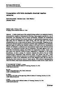
A Petri-net is a bipartite oriented (weighted) graph of transitions, usually represented as square boxes, and places, usually represented as circles, that defines a (actually not only one) transition relation on markings of the net, i.e. multisets of tokens associated to places. The relation is defined by firings of transitions, i.e. when there are tokens (as many as the weight of the incoming arc) in all pre-places of a transition, they can be consumed and as many tokens as the weight on the outgoing arc are added to each post-place. The classical Petri-net view of a reaction model is simply to associate biochemical species to places and biochemical reactions to transitions. Example 1 For instance the enzymatic reaction written (in BIOCHAM-like syntax), A + E A-E => B + E corresponds to the Petri-net depicted in figure 1.
E
t1 A
A-E
t2
B
t−1 Figure 1: Petri-net corresponding to the biochemical model of example 1
In this Petri-net, starting from a marking with at least one token in A and in E, one can remove one of each to produce one token in A-E (firing of t1 ) and then either remove it to add again one token to A and one to E (firing of t−1 ), or to add one B and one E (firing of t2 ). P (resp. T) invariants are defined, as usual, as vectors V representing a multiset of places (resp. of transitions) such that V · I = 0 (resp. I · V = 0) where I is the incidence matrix of the Petri net, i.e. Ii j is the number of arcs from transition i to place j, minus the number of arcs from place j to transition i. Intuitively, a P-invariant is a multiset representing a weighting of the places and such that any such weighted marking remains invariant by any firing; a T-invariant represents a multiset of firings that will leave invariant any marking (see also section 6). As explained in introduction, for reaction models these invariants are used for flux analysis, variable simplification through conservation law extraction, module decomposition, etc. More precisely, invariants, being based on the structure, provide of course qualitative information that can be used for instance for model-checking (e.g. reachability analysis). It is however interesting to note that some non-trivial quantitative information is also captured. For instance a semi-positive P-invariant defines a (quantitative) conservation law, whatever the dynamics of the system. Note that there are other ones, like the following when k1 = k2:
MA(k1) for A => A + B. MA(k2) for A => _. Where MA(k) denotes that the kinetics of the reaction follow the Mass Action law with rate k. The resulting ODEs would have the following property: d[A] + [B] = −k2 ∗ [A] + k1 ∗ [A] = (k1 − k2 ) ∗ [A] dt In the same manner, as pointed out in section 2 links have been found between the structure of the graph and the dynamical behavior (through positive and negative cycles in the influence graph or CRNT) from the structure of the reaction model. There is also information lying between quantitative and qualitative, like the definition of modules from T-invariants as explored recently in [13, 14], and to sum this up, the structure of the reaction model contains information that can be used at any abstraction level.
5
Related work
To compute the invariants of a Petri net, especially if this computation is combined with other Petri-net analyses, like sinks and sources, traps, deadlocks, etc. the most natural solution is to use a Petri-net dedicated tool like INA, PiNA, or Charlie for instance through the interface of Snoopy [15], which will soon allow the import of SBML models as Petri-nets. Standard integer methods like Fourier-Motzkin elimination will then provide an efficient means to compute P or T-invariants. These methods however generate lots of candidates which are afterwards eliminated and also need to incorporate some means (like equality class definition) to avoid combinatorial explosion at least in some simple cases, as explained in section 7. Another way to extract the minimal semi-positive invariants of a model is to use one of the software tools that provide this computation for biological systems, generally as “conservation law” computation, and based on linear algebra methods like QR factorization [31]. This is the case for instance of the METATOOL [32] and COPASI [16] tools. The idea is to use a linear relaxation of the problem, which suits well very big graphs, but needs again a
posteriori filtering of the candidate solutions. Moreover, these methods do not incorporate any means of symmetry elimination (see section 7).
6
Finding invariants as a Constraint Solving Problem
We will illustrate our new method for computing the invariants with the case of P-invariants (but T-invariants, being dual, work in the same fashion). For a Petri net with p places and t transitions (Li → Ri ), a P-invariant is a vector V ∈ N p s.t. V · I = 0, i.e. ∀1 ≤ i ≤ t V · Li = V · Ri . Since those vectors all live in N p , it is quite natural to see this as a Constraint Solving Problem (CSP) with t (linear) equality constraints on p Finite Domains variables. Example 2 Using the Petri-net of example 1 we have:
A + E => A-E A-E => A + E A-E => B + E This results in the following equations: A+E AE AE
= AE = A+E = B+E
(1) (2) (3)
where obviously equation (2) is redundant. The task is actually to find invariants with minimal support (a linear combination of invariants belonging to N p also being an invariant), i.e. having as few non-zero components as possible, these components being as small as possible, but of course non trivial, we thus add the constraint that V · 1 > 0. Example 3 In our running example we thus add A + E + AE + B > 0. Now, to ensure minimality the labelling is invoked from small to big values and a branch and bound procedure is wrapped around it, maintaining a partial base B of P-invariant vectors and adding the constraint that a new vector V is solution if ∀B ∈ B ∏Bi 6=0 Vi = 0, which means that its support is not bigger than that of any vector of the base. Unfortunately, even with the last constraint, no search heuristic was found that makes removing subsumed Pinvariants unnecessary. Thus, if a new vector is added to B, previously found vectors with a bigger support must be removed. This algorithm was implemented directly into BIOCHAM [3], which is programmed in GNU-Prolog, and allowed for immediate testing. Example 4 In our running example we find two minimal semi-positive P-invariants: • E = AE = 1 and A = B = 0 • A = B = AE = 1 and E = 0
7
Equality classes
7.1
A hard problem
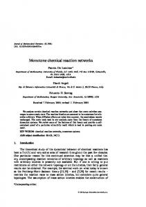
The problem of finding minimal semi-positive invariants clearly suffers from a computational blowup since there can be an exponential number of such invariants. For instance the model given in example 5 has 2n minimal semi-positive P-invariants (each one with either Ai or Bi equal to 1 and the other equal to 0). Example 5 The model:
A1 + B1 => A2 + B2 A2 + B2 => A3 + B3 ... An + Bn => A1 + B1 is depicted in figure 2
A1
A2
A3
An ...
B1
B2
B3
Bn
Figure 2: Example net with 2n minimal semi-positive P-invariants
7.2
CSP-like Symmetry breaking
A first remark is that in this example, there is a variable symmetry [12] between all the pairs (Ai , Bi ) of variables corresponding to places. This symmetry is easy to detect (purely syntactical) and can be eliminated through the usual ordering of variables, by adding the constraints Ai ≤ Bi . This classical CSP optimization is enough to avoid most of the trivial exponential blow-ups and corresponds to the initial phase of parallel places detection and merging of the equality classes optimization for the standard Fourier-Motzkin algorithm [21]. Note however that in that method, classes of equivalent variables are detected and eliminated before and during the invariant computation, which would correspond to local symmetry detection and was not implemented in our prototype. Moreover, in [21], equality class elimination is done through replacement of the symmetric places by a representative place. The full method reportedly improves by a factor two the computation speed. Even if in the context of the original article this is done only for ordinary Petri-nets (only one edge from one place to a transition and from one transition to one place), we can see that it can be even more efficient to use this replacement technique in our case: Example 6 ... A + B => 4*C ... Instead of simply adding A ≤ B to our constraints, which will lead to 3 solutions when C = 1 before symmetry expansion: (A, B) ∈ {(0, 4), (1, 3), (2, 2)}, replacing A and B by D will reduce to a single solution D = 4 before expansion of the subproblem A + B = D. This partial detection of independent subproblems, which can be seen as a complex form of symmetry identification, can once again be done syntactically at the initial phase, and can be stated as follows: replace ∑i ki ∗ Ai by a single variable A if all the Ai occur only in the context of this sum i.e. in our Petri net all pre-transitions of Ai are connected to Ai with ki edges and to all other A j with k j edges and same for post-transitions. For a better constraint propagation, another intermediate variable can be introduced such that A = gcd(ki ) · A0 . In our experiments the simple case of parallel places (i.e. all ki equal to 1 in the sum) was however the one encountered most often. 7.3
Going farther
In our Nicotine tool (available at http://contraintes.inria.fr/~soliman/nicotine/), we extended SBML support to also include APNN and PNML import/export. We then proceeded to add one more step of optimization. The point is to note that if a place (in the case of P-invariants) P has only one single input transition I and one single output transition O, and if there exists a path between I and O such that it goes only through such places (with single input and output) Pi , whatever the intermediate transitions, then there is a bijection between minimal semi-positive P-invariants such that P > 0 and those where P = 0 and min(Pi ) > 0. It is thus possible to look only for solutions where P = 0 and to obtain the other ones by “symmetry”. Actually this bijection consists in mapping all Pi to Pi − min(Pi ) and P from 0 to min(Pi ). Intuitively the “flow” going through the Pi is redirected through P. More precisely, for the intermediate transitions we get equations of the form Pj + · · · = Pj+1 + · · ·, which are unchanged by our bijection, and for I (resp. O), P replaces the first (resp. last) Pi . The bijection only maps minimal invariants to minimal invariants (since at least one of the Pi gets removed from the support when P gets added and reciprocally).
8
Example, the MAPK Cascade
The MAPK signal transduction cascade is a well studied system that appears in lots of organisms and is very important for regulating cell division [27]. It is composed of layers, each one activating the next, and in detailed
models shows two intertwined pathways conveying EGF and NGF signals to the nucleus. A simple MAPK cascade model, that of [22] without scaffold, is used here as an example to show the results of P-invariant computation. rule_1
RAF-RAFK
rule_21
RAF~{p1}
RAFK
rule_3
rule_5
RAFPH-RAF~{p1}
rule_24
rule_2
rule_4
MEK~{p1}
MEK-RAF~{p1}
rule_22
rule_6
RAFPH
RAF
rule_7
MEK~{p1}-RAF~{p1}
rule_23
rule_8
MEK~{p1,p2}
rule_13
rule_11
MAPK-MEK~{p1,p2}
rule_14
MEKPH-MEK~{p1,p2}
rule_27
rule_12
MAPK~{p1}
rule_26
MEKPH
rule_15
rule_9
MAPK~{p1}-MEK~{p1,p2}
rule_16
MEKPH-MEK~{p1}
rule_28
rule_10
MAPK~{p1,p2}
rule_25
MEK
rule_19
MAPKPH-MAPK~{p1,p2}
rule_30
rule_20
MAPKPH
rule_17
MAPKPH-MAPK~{p1}
rule_18
rule_29
MAPK
Figure 3: 3 of the 7 P-invariants found in the MAPK cascade model of [22]. The blue one (RAF), the pink one (MEK) and the green one (MAPK) with intersections in purple (blue+pink) and khaki (pink+green).
Seven minimal semi-positive P-invariants are found almost instantly: RAFK, RAFPH, RAF, MEKPH, MEK, MAPKPH, MAPK. Three of them are depicted in figure 3, the full list is given in table 1. RAFK, RAF-RAFK RAFPH, RAFPH-RAF∼{p1} RAF, MEK-RAF∼{p1}, RAF-RAFK, RAFPH-RAF∼{p1}, MEK∼{p1}-RAF∼{p1}, RAF∼{p1} MEKPH, MEKPH-MEK∼{p1}, MEKPH-MEK∼{p1, p2} MEK, MAPK-MEK∼{p1, p2}, MEK-RAF∼{p1}, MEKPH-MEK∼{p1}, MEKPH-MEK∼{p1, p2}, MAPK∼{p1}-MEK∼{p1, p2}, MEK∼{p1}-RAF∼{p1}, MEK∼{p1}, MEK∼{p1, p2} MAPKPH, MAPKPH-MAPK∼{p1}, MAPKPH-MAPK∼{p1, p2} MAPK, MAPK-MEK∼{p1, p2}, MAPKPH-MAPK∼{p1}, MAPK∼{p1, p2} MAPK∼{p1}-MEK∼{p1, p2}, MAPK∼{p1}, MAPKPH-MAPK∼{p1, p2}, Table 1: P-invariants of the MAPK cascade model of [22]
Note that these 7 P-invariants define 7 algebraic conservation rules and thus decrease the size of the corresponding ODE model from 22 variables and equations to only 15.
9
Evaluation on other examples
Schoeberl’s model is a more detailed version of the MAPK cascade, which is quite comprehensive [28], but too big to be studied by hand. It can however be easily broken down into fourteen more easily understandable units formed by P-invariants, as shown in table 2, along other examples representing amongst the biggest reaction networks publicly available in Systems Biology. All the curated models in the December 2008 release of biomodels.net were also tested and none of them required more than 1s to compute all its minimal P-invariants. All the Petri-nets of www.petriweb.org were also tested, though they do not correspond to reaction models, only one took more than 1s: model 1516, which took about 3s to compute 1133 minimal P-invariants. We think that the structure of this kind of net is however very different from that of usual biochemical reaction models and intend to explore this distinction further in the future. We could not compare our results with those provided in [31] since the models they use, coming from metabolic pathways flux analyses, do not have an integer stoichiometry matrix, however the examples of table 2 show the feasibility of P-invariant computation by constraint programming for quite big networks. Note that for networks of this size, the upper bound of the domain of variables had to be set manually (to a reasonable value like 8 since actually only 2 or 3 was needed in all the biological models we have encountered up to now). Otherwise, the only over-approximation of the upper bound found was the product of the l.c.m. of stoichiometric coefficients of each reaction, which explodes really fast and leads to unnecessarily long computation. We thereby lose completeness, but it is not enforced either by QR-factorization methods, and does not seem to miss anything on real life examples.
10
Conclusion
After the genome sequencing, building and correcting System Biology models is a new and rich domain where lots of mathematics and computer science tools can be used. We argue that to encompass the heterogeneity of the available data it is necessary to provide formal languages for different levels of abstractions and to relate them precisely [9] but also to formalize the properties of the studied system in order to leverage all the automatic tools from machine learning and optimization. This amounts to more initial work for the modeller who should now both represent his system as a set of reactions but also the experimental data available (either directly in temporal logic or through tools that will extract such Model Schoeberl’s MAPK [28] Curie’s E2F/Rb [4] Kohn’s map [20]
transit. 125 ∼500
places 105 ∼400
P-invar. 14 79
∼800
∼500
65
Invariant size from 2 to 44 from size 1 (EP300) to about 230 (E2F1 box) from size 1 (Myt1) to about 200 (pRb or cdk2)
Table 2: Minimal semi-positive P-invariant computation on bigger models of biochemical reaction networks, all < 1s
specification from other kinds of data like, for instance time series). However after this initial step, lots of different tools, which will complement simulation, become available to automatically curate, refine, modularize, . . . his model. In the BIOCHAM environment we have implemented some of the tools we thought most useful from the modelling point of view, but through SBML import/export it is also possible to rely on the vast body (see http://www.sbml. org for a list) of software handling reaction-based biochemical models. The crucial point here is the multiple abstraction levels that can be used to reason about a single reaction model. We have illustrated this point through invariant computation. We have shown that P-invariants of a biological reaction model are not difficult to compute in most cases. They do however carry information about conservation laws that are useful for efficient and precise dynamical simulation of the system, and provide some notion of module, which is related to the life cycle of molecules. T-invariants are already used more commonly, and get more and more focus recently. We introduced a new method to efficiently compute P and T-invariants of a reaction network, based on Finite Domain constraint programming. It includes symmetry detection and breaking and scales up well to the biggest reaction networks found. The idea of applying constraint based methods to classical problems of the Petri-net community is not new, but seems currently mostly applied to the model-checking. We argue that structural problems (invariants, sinks, attractors, etc.) can also benefit from the know-how developed for finite domain CP solving, like symmetry breaking, search heuristics, etc. and thus intend to generalize our approach to other problems of this category, hoping to bring more and more qualitative and quantitative information from the pure structure of the reaction models.
11
References
[1] Antoniotti, M., Policriti, A., Ugel, N., and Mishra, B. Cell Biochemistry and Biophysics 38, 271–286 (2003). [2] Calzone, L., Chabrier-Rivier, N., Fages, F., and Soliman, S. In Transactions on Computational Systems Biology VI, Plotkin, G., editor, volume 4220 of Lecture Notes in BioInformatics, 68–94. Springer-Verlag November (2006). CMSB’05 Special Issue. [3] Calzone, L., Fages, F., and Soliman, S. BioInformatics 22(14), 1805–1807 (2006). [4] Calzone, L., Gelay, A., Zinovyev, A., Radvanyi, F., and Barillot, E. Molecular Systems Biology 4(173) (2008). [5] Chabrier-Rivier, N., Chiaverini, M., Danos, V., Fages, F., and Schächter, V. Theoretical Computer Science 325(1), 25–44 September (2004). [6] Chickarmane, V., Kholodenkob, B. N., and Sauro, H. M. Journal of Theoretical Biology 244, 68–76 (2007). [7] Danos, V. and Laneve, C. Theoretical Computer Science 325(1), 69–110 (2004). [8] Eker, S., Knapp, M., Laderoute, K., Lincoln, P., Meseguer, J., and Sönmez, M. K. In Proceedings of the seventh Pacific Symposium on Biocomputing, 400–412, January (2002). [9] Fages, F. and Soliman, S. Theoretical Computer Science 403(1), 52–70 (2008). [10] Fages, F. and Soliman, S. In Proceedings of Formal Methods in Systems Biology FMSB’08, number 5054 in Lecture Notes in Computer Science. Springer-Verlag, February (2008). [11] Fages, F., Soliman, S., and Chabrier-Rivier, N. Journal of Biological Physics and Chemistry 4(2), 64–73 October (2004). [12] Freuder, E. C. In Proceedings of AAAI’91, 227–233. MIT Press, (1991). [13] Gilbert, D., Heiner, M., and Lehrack, S. In CMSB’07: Proceedings of the fifth international conference on Computational Methods in Systems Biology, volume 4695 of Lecture Notes in Computer Science. SpringerVerlag, (2007). [14] Grafahrend-Belau, E., Schreiber, F., Heiner, M., Sackmann, A., Junker, B. H., Grunwald, S., Speer, A., Winder, K., and Koch, I. BMC Bioinformatics 9(90) February (2008). [15] Heiner, M., Richter, R., and Schwarick, M. In Procedings of the International Workshop on Petri Nets Tools and APplications (PNTAP 2008) (ACM Digital Library, Marseille, 2008). to appear. [16] Hoops, S., Sahle, S., Gauges, R., Lee, C., Pahle, J., Simus, N., Singhal, M., Xu, L., Mendes, P., and Kummer, U. BioInformatics 22(24), 3067–3074 (2006). [17] Hucka, M. et al. Bioinformatics 19(4), 524–531 (2003). [18] Ideker, T., Galitski, T., and Hood, L. Annual Review of Genomics and Human Genetics 2, 343–372 (2001). [19] Kanehisa, M. and Goto, S. Nucleic Acids Research 28(1), 27–30 (2000). [20] Kohn, K. W. Molecular Biology of the Cell 10(8), 2703–2734 August (1999). [21] Law, C. F., Gwee, B. H., and Chang, J. IEE Proceedings: Computers and Digital Techniques 1(5), 612–624 (2007). [22] Levchenko, A., Bruck, J., and Sternberg, P. W. PNAS 97(11), 5818–5823 May (2000). [23] Phillips, A. and Cardelli, L. Transactions on Computational Systems Biology (to appear). Special issue of BioConcur 2004. [24] Reddy, V. N., Mavrovouniotis, M. L., and Liebman, M. N. In Proceedings of the 1st International Conference
[25] [26]
[27] [28] [29] [30] [31] [32]
on Intelligent Systems for Molecular Biology (ISMB), Hunter, L., Searls, D. B., and Shavlik, J. W., editors, 328–336. AAAI Press, (1993). Regev, A., Silverman, W., and Shapiro, E. Y. In Proceedings of the sixth Pacific Symposium of Biocomputing, 459–470, (2001). Rizk, A., Batt, G., Fages, F., and Soliman, S. In CMSB’08: Proceedings of the fourth international conference on Computational Methods in Systems Biology, Heiner, M. and Uhrmacher, A., editors, volume 5307 of Lecture Notes in Computer Science, 251–268. Springer-Verlag, October (2008). Roovers, K. and Assoian, R. K. BioEssays 22(9), 818–826 August (2000). Schoeberl, B., Eichler-Jonsson, C., Gilles, E., and Muller, G. Nature Biotechnology 20(4), 370–375 (2002). Schuster, S., Fell, D. A., and Dandekar, T. Nature Biotechnology 18, 326–332 (2002). Thomas, R., Gathoye, A.-M., and Lambert, L. European Journal of Biochemistry 71(1), 211–227 December (1976). Vallabhajosyulaa, R. R., Chickarmane, V., and Sauro, H. M. BioInformatics November (2005). Advance Access. von Kamp, A. and Schuster, S. Bioinformatics 22(15), 1930–1931 (2006).