Mar 31, 2014 - equate optimization of baker's yeast production in the food industry. ... of the partner Puratos (world leader in bakery, pastry, and chocolate).
Modelling, Optimization and Control of Yeast Fermentation Processes in Food Industry Anne Richelle
Ph.D. Thesis submitted at the
cole polytechnique de Bruxelles Université libre de Bruxelles and presented on 31th March, 2014 in fulfillment of the requirements for the degree of
Docteur en Sciences de l’Ingénieur
Jury members Pr. Dr. Ir. M. Kinnaert Pr. Dr. Ir. F. Debaste Pr. Dr. Ir. A. Vande Wouwer Pr. Dr. Ir. J. Van Impe Pr. Dr. J.-M. Sablayrolles
Univeristé Libre de Bruxelles - President Université Libre de Bruxelles - Secretary Université de Mons Katholieke Universiteit Leuven INRA Montpellier, France
Pr. Dr. Ir. Ph. Bogaerts
Université Libre de Bruxelles - Thesis Advisor
Chaque porte passée est une fenêtre ouverte sur le reste avenir...
Remerciements Mes premiers remerciements s’adressent au Fonds pour la formation à la Recherche dans l’Industrie et dans l’Agriculture et au Fonds David & Alice Van Buuren qui ont financé cette thèse de doctorat. Je tiens également à remercier Coralie Lefebvre, Bernard Genot et Sylvestre Awono, nos collaborateurs industriels de Puratos qui ont contribué à la mise en perspective de ces recherches dans un contexte industriel. Je tiens à souligner l’investissement des mémorants avec qui j’ai eu l’occasion de travailler sur certaines parties de cette thèse: Sergio Gutiérrez, Nicolas Marquet, Guevork Mikaelian et Martina Tomassini. Je remercie Jean Louis Van Pee, Laurent Catoire et Serge Torfs pour l’aide technique qu’ils m’ont apportée dans le cadre de la mise en place des installations expérimentales; Laurent Dewasme dont les conseils avisés m’ont permis d’élargir mes réflexions; la Professeure Laurence Van Nedervelde et Roxane Van Heurck pour les relectures de cette thèse; tous les membres du service 3BIO qui ont subi mes blagues à trois francs six sous pendant de nombreuses années et plus particulièrement Nathalie, Danièle, Jean-Marc, Zakaria, Khadija et Marie sans oublier mon cher Alex; et bien évidement tous les amis sur qui j’ai pu compter durant ces cinq dernières années: ils ont largement contribué à mon sourire quotidien! Je n’aurais jamais pu réaliser cette thèse sans le soutien inconditionnel de ma famille: François, Marie, ma mère et mon père. Je ne saurais jamais assez les remercier d’être toujours là pour moi. Last but not least, il est celui sans qui rien de tout cela n’aurait pu voir le jour et sans nulle doute ma plus belle rencontre universitaire: le Professeur Philippe Bogaerts. Grâce à son exigence, j’ai acquis des qualités qui m’ont longtemps fait défaut: la rigueur et la patience. Il m’a toujours poussée à me dépasser et à donner le meilleur de moi-même. A mes yeux, il est devenu bien plus qu’un simple promoteur et je lui dois en grande partie d’être celle que je suis aujourd’hui. Je n’ai pas de plus grande fierté que celle d’avoir pu travailler durant six ans à ses côtés. Philippe, un merci ne suffirait pas!
Contents 1 Introduction 1.1 Context and Motivations . . . . . . . . . . . . . . . . . . . . . 1.2 Objectives . . . . . . . . . . . . . . . . . . . . . . . . . . . . . 1.3 Organization of the Manuscript . . . . . . . . . . . . . . . . .
17 17 21 22
2 Baker’s Yeast Production 2.1 Introduction . . . . . . . . . . . . . . . . . . . . . . . . . 2.2 Saccharomyces cerevisiae: a Model Organism . . . . . . 2.2.1 History . . . . . . . . . . . . . . . . . . . . . . . 2.2.2 Nutrition and Growth Conditions . . . . . . . . . 2.2.3 Main Metabolic Reactions . . . . . . . . . . . . . 2.2.3.1 Central Carbon Metabolism . . . . . . 2.2.3.2 Central Nitrogen Metabolism . . . . . 2.2.3.3 Storage Carbohydrates Metabolism . . 2.3 Industrial Production Process . . . . . . . . . . . . . . 2.3.1 Baking Characteristics . . . . . . . . . . . . . . 2.3.2 Medium Composition . . . . . . . . . . . . . . . 2.3.3 Bioreactor Description: Monitoring and Control 2.3.4 Process Operating Conditions . . . . . . . . . .
. . . . . . . . . . . . .
. . . . . . . . . . . . .
. . . . . . . . . . . . .
25 25 26 27 28 31 32 36 37 39 41 42 44 46
3 Modelling of Bioprocesses 3.1 Introduction . . . . . . . . . . . . . . . . . . . . . . . . 3.2 Simulation and Modelling . . . . . . . . . . . . . . . . 3.2.1 What Kind of Models? . . . . . . . . . . . . . . 3.2.2 Macroscopic Modelling . . . . . . . . . . . . . 3.2.2.1 Reaction Scheme . . . . . . . . . . . 3.2.2.2 Kinetic Expression . . . . . . . . . . . 3.2.2.3 Mass Balance Equations . . . . . . . 3.3 Parameter Estimation . . . . . . . . . . . . . . . . . . 3.3.1 Experimental Database . . . . . . . . . . . . . 3.3.2 Identification Criterion and Algorithm . . . . 3.4 Validation of the Model . . . . . . . . . . . . . . . . . 3.4.1 Direct and Cross-validation Tests . . . . . . . . 3.4.2 Uncertainty Analysis . . . . . . . . . . . . . . . 3.4.2.1 Parameter Uncertainty . . . . . . . . 3.4.2.2 Predicted Model Output Uncertainty
. . . . . . . . . . . . . . .
. . . . . . . . . . . . . . .
. . . . . . . . . . . . . . .
49 49 51 51 53 53 54 56 59 59 61 64 65 66 66 69
. . . . . . . . . . . . . . .
1
Contents 3.5
Model of Sonnleitner and K¨ appeli
. . . . . . . . . . . . . . .
72
4 Materials and Methods 4.1 Microorganism and Medium Composition . . . . . . . . . . 4.2 Bioreactor Description . . . . . . . . . . . . . . . . . . . . . 4.3 Inoculum Development and Experimental Conditions . . . 4.4 Analytical Methods . . . . . . . . . . . . . . . . . . . . . .
. . . .
5 Modelling the Link between N and C Source Uptakes 5.1 Introduction . . . . . . . . . . . . . . . . . . . . . . . . . . 5.2 Model-based Design of the Experimental Database . . . . 5.3 Modelling of Coordinated Uptake of N and C Sources . . 5.4 Parametric Estimation and Validation of the Model . . . 5.4.1 Uncertainty Analysis on Predicted Model Outputs 5.5 Conclusion . . . . . . . . . . . . . . . . . . . . . . . . . .
83 . 83 . 84 . 88 . 93 . 103 . 106
. . . . . .
77 77 77 78 80
6 Modelling the Oxygen Dynamics 6.1 Introduction . . . . . . . . . . . . . . . . . . . . . . . . . . . . 6.2 Theoritical Framework . . . . . . . . . . . . . . . . . . . . . . 6.3 General Procedure for Introduction of Oxygen into the Model 6.3.1 Step 1: Transfer Coefficient Estimation . . . . . . . . 6.3.2 Step 2: Pseudo-stoichiometric Parameter Estimation 6.3.3 Step 3: Kinetic Parameters Estimation . . . . . . . . . 6.4 Conclusion . . . . . . . . . . . . . . . . . . . . . . . . . . . .
107 107 108 111 112 128 131 138
7 Model Extensions: Intracellular Metabolite Production 7.1 Introduction . . . . . . . . . . . . . . . . . . . . . . . . 7.2 Modelling Trehalose Production . . . . . . . . . . . . . 7.2.1 Identification with the First Set of Experiments 7.3 Modelling Glycogen Production . . . . . . . . . . . . . 7.3.1 Identification with the First Set of Experiments 7.4 Conclusion . . . . . . . . . . . . . . . . . . . . . . . .
. . . . . .
. . . . . .
. . . . . .
. . . . . .
139 139 140 141 143 143 146
8 Off-line Process Optimization and Control Strategies 8.1 Introduction . . . . . . . . . . . . . . . . . . . . . . . 8.2 Dynamic Optimization Techniques . . . . . . . . . . 8.3 Optimization Criteria and Procedure . . . . . . . . . 8.3.1 CVP Approach with Mesh Refinement . . . . 8.3.2 Mathematical Analysis of Optimal Operation 8.4 Comparison of the Two Approaches . . . . . . . . . 8.5 Conclusion . . . . . . . . . . . . . . . . . . . . . . .
. . . . . . .
. . . . . . .
. . . . . . .
. . . . . . .
147 147 148 150 151 154 165 176
. . . . . . .
9 General Conclusions and Perspectives 177 9.1 General Conclusions . . . . . . . . . . . . . . . . . . . . . . . 177 9.2 Suggestions for Future Research . . . . . . . . . . . . . . . . . 180
2
Contents Bibliography
183
Appendices
191
1 - General Kinetic Model of the Nitrogen Uptake Rate
193
2 - Influence of the β Factor
201
3 - Recorded Data Associated to the P O2 Measurements
205
4 - Second Step of the pO2 Procedure
211
5 - Cross-validation of the Complete Model
213
6 - Influence of Mesh Refinement in the CVP Approach
223
7 - Influence of λ Values on Optimization Results
225
8 - Optimal solutions including Trehalose and Glycogen
231
3
List of Figures 2.1 2.2 2.3
Central Carbon Metabolism (Raven et al., 2007) . . . . . . . Central Nitrogen Metabolism (ter Schure et al., 2000) . . . . Schematic representation of a bioreactor . . . . . . . . . . . .
35 37 46
3.1
Schematic representation of “overflow metabolism” . . . . . .
74
5.1 5.2 5.3 5.4 5.5 5.6 5.7 5.8 5.9 5.10
Ethanol time profile imposed for the 4 experiments . . . . . . 84 Culture medium feeding profile imposed for the 4 experiments 85 Sonnleitner & K¨ appeli’s model and experimental measurements 86 Correlation matrix of the identified parameters (dimθ = 17) . 95 Correlation matrix of the identified parameters (dimθ = 15) . 97 Model simulation of the non-measured variable α-ketoglutarate 100 Direct validation of the model - Exp. 1-4 . . . . . . . . . . . 101 Leave-one-out cross-validation of the model - Exp. 1-4 . . . . 102 Local approach for uncertainty analysis - Exp. 1-4 . . . . . . 104 Global approach for uncertainty analysis - Exp. 1-4 . . . . . . 105
6.1 6.2 6.3 6.4 6.5 6.6 6.7 6.8 6.9 6.10 6.11 6.12 6.13 6.14 6.15 6.16
Schematic representation of “film theory gas transfer” . . . . Recorded data associated to pO2 measurements - Exp. 4 . . . 1st kL a estimation: direct validation of OTR reproduction . . 1st kL a estimates evolution over the time for each experiment Data obtained after pre-treatement . . . . . . . . . . . . . . . 2nd kL a estimation: direct validation of OTR reproduction . 2nd kL a estimates evolution over the time for each experiment Data obtained after a sampling of pO2 measurements . . . . . 3th kL a estimation: direct validation of OTR reproduction . . 3th kL a estimates evolution over time for each experiment . . 4th kL a estimation: direct validation of OTR reproduction . . 4th kL a estimates evolution over time for each experiment . . Dissolved oxygen measurements reproduction . . . . . . . . . Correlation matrix of the identified parameters (dimθ = 18) . Direct validation of complete model - Exp. 1-4 . . . . . . . . Direct validation of complete model - Exp. 1bis-4bis . . . . .
7.1 7.2 7.3
Direct validation of trehalose model extension - Exp. 1-4 . . . 142 Cross-validation of trehalose model extension - Exp. 1-4 . . . 142 Direct validation of glycogen model extension - Exp. 1-4 . . . 145
111 115 117 118 119 120 121 122 123 124 126 127 130 133 135 136
5
List of Figures 7.4
Cross-validation of glycogen model extension - Exp. 1-4 . . . 145
8.1 8.2 8.3 8.4 8.5 8.6 8.7 8.8 8.9 8.10 8.11 8.12 8.13
Comparison of 3 optimal results obtained with CVP approach 153 States and feeding of 76 S.-A. optimal solutions . . . . . . . . 161 Distribution of the parameters of 76 S.-A. optimal solutions . 162 Influence of E min set for the definition of t2 on Xmax . . . . 163 CVP and S.-A. optimal solutions comparison - State . . . . . 165 CVP and S.-A. optimal solutions comparison - Feeding . . . . 166 CVP solution and measurements comparison - 1st Exp. . . . 167 Identification results and measurements comparison - 1st Exp. 168 CVP and S.-A. comparison with sample volumes - State . . . 169 CVP and S.-A. comparison with sample volumes - Feeding . . 170 CVP solution and measurements comparison - 2nd Exp. . . . 171 Identification results and measurements comparison - 2nd Exp. 173 Global approach for uncertainty analysis - CVP solution . . . 174
9.1 9.2
Direct validation - Generalized nitrogen kinetic - Exp. 1-4 . . 197 Cross-validation - Generalized nitrogen kinetic - Exp. 1-4 . . 198
9.3
Comparison of 3 direct validations with different β values . . 203
9.4 9.5 9.6 9.7 9.8 9.9 9.10 9.11
Recorded Recorded Recorded Recorded Recorded Recorded Recorded Recorded
data data data data data data data data
associated associated associated associated associated associated associated associated
to to to to to to to to
pO2 pO2 pO2 pO2 pO2 pO2 pO2 pO2
measurements measurements measurements measurements measurements measurements measurements measurements
-
Exp. Exp. Exp. Exp. Exp. Exp. Exp. Exp.
1bis 2bis 3bis 4bis 1. . 2. . 3. . 4. .
. . . . . . . .
206 206 207 207 208 208 209 209
9.12 Dissolved oxygen measurements reproduction . . . . . . . . . 212 9.13 9.14 9.15 9.16 9.17 9.18 9.19 9.20
First cross-validation of the model - Exp. 1-4 . . . . First cross-validation of the model - Exp. 1bis-4bis Second cross-validation of the model - Exp. 1-4 . . . Second cross-validation of the model - Exp. 1bis-4bis Third cross-validation of the model - Exp. 1-4 . . . . Third cross-validation of the model - Exp. 1bis-4bis Fourth cross-validation of the model - Exp. 1-4 . . . Fourth cross-validation of the model - Exp. 1bis-4bis
. . . . . . . . . . . . . . . . . . . . . . . . . . . . . .
. . . . . . . .
214 215 216 217 218 219 220 221
9.21 States and feeding of 40 S.-A. optimal solutions . . . . . . . . 226 9.22 Distribution of the parameters of 76 S.-A. optimal solutions . 227 9.23 Comparison of optimal solutions by fixing λG and λN . . . . 228 9.24 Optimal solutions for trehalose and glycogen - 1st experiment 231
6
List of Figures 9.25 Optimal solutions for trehalose and glycogen - 2nd experiment 231
7
List of Tables 2.1 2.2 2.3 2.4
The elemental composition of baker’s yeast . . . Defined medium for cultivation of baker’s yeast . Medium composition for baker’s yeast production Typical molasses composition . . . . . . . . . . .
. . . .
. . . .
. . . .
. . . .
. . . .
. . . .
. . . .
29 30 42 43
3.1
Parameter values of Sonnleitner and K¨appeli’s model . . . . .
75
5.1 5.2 5.3
Identification of the model (dimθ = 17) - Exp. 1-4 . . . . . . 96 Identification of the model (dimθ = 15) - Exp. 1-4 . . . . . . 98 Confidence intervals for identified parameter values - Exp. 1-4 99
6.1 6.2 6.3 6.4 6.5 6.6
1st parameter identification (dimθ = 5) - kL a correlation . . . 2nd parameter identification (dimθ = 5) - kL a correlation . . 3th parameter identification (dimθ = 5) - kL a correlation . . 4th parameter identification (dimθ = 2) - kL a correlation . . Identification of yield coefficients (dimθ = 3) - 6 experiments Identification of the model (dimθ = 18) - Exp. 1-4/1bis-4bis .
7.1 7.2
Identification of trehalose model extension (dimθ = 3) . . . . 141 Identification of glycogen model extension (dimθ = 3) . . . . 144
8.1 8.2 8.3
Optimization results - Multistart S.-A. . . . . . . . . . . . . . 161 Optimization results with sample volumes - Multistart S.-A. 169 Identification of the model (dimθ = 15) - 2nd Exp. . . . . . . 172
9.1 9.2 9.3
Identification of the generalized model (dimθ = 17) - Exp. 1-4 195 Identification of the generalized model (dimθ = 16) - Exp. 1-4 196 Comparison of kinetic expression of nitrogen uptake rate . . . 199
9.4
Influence of the β factor on parameter identification results . 202
9.5
Identification of yield coefficients (dimθ = 3) - 6 experiments
9.6 9.7
Influence of the initial number of feeding partitions . . . . . . 223 Influence the number of refinement iterations . . . . . . . . . 223
9.8 9.9
Optimization results (dimθ = 6) - Multistart S.-A. . . . . . . 226 Comparison of optimization results by fixing λG and λN . . . 228
117 120 123 125 129 134
212
9
List of symbols a
“operating” parameter
A
α-ketoglutarate concentration in cell [g gX −1 ]
AIRF
rate of the gas input flow (airflow) [slpm]
b
“operating” parameter
c
“operating” parameter
ci
concentration of dissolved gas i in equilibrium with its partial pressure in the gas [mol L−1 ]
COR
correlation matrix
d
“operating” parameter
D
dilution rate [h−1 ]
E
ethanol concentration in bioreactor [g L−1 ]
Fi
volumetric feeding rate of component ξi [L h−1 ]
Fin
volumetric feeding rate [L h−1 ]
Fout
volumetric outlet rate [L h−1 ]
G
glucose concentration in bioreactor [g L−1 ]
Gin
glucose concentration in feeding medium [g L−1 ]
Gin
molar gas inflow rate [mol h−1 ]
Gout
molar gas outflow rate [mol h−1 ]
GLY
glycogen concentration in cell [g gX −1 ]
Hi
Henry coefficient [L P a mol−1 ]
J(θ)
identification criterion
ki
pseudo-stoichiometric coefficient [g g −1 ]
kL a
transfer coefficient of oxygen from gas to liquid [h−1 ]
Kξ i
saturation constant [g L−1 ]
KG
Monod constant of glucose [g L−1 ]
11
List of Tables KO
Monod constant of oxygen [g L−1 ]
KE
Monod constant of ethanol [g L−1 ]
KN
Monod constant of nitrogen [g L−1 ]
KA
Monod constant of α-ketoglutarate [g L−1 ]
KIξi
inhibition constant [g L−1 ]
KI
ethanol inhibition constant [g L−1 ]
KIA
α-ketoglutarate inhibition constant of glucose uptake rate [g L−1 ]
KIA2
α-ketoglutarate inhibition constant of nitrogen uptake rate[g L−1 ]
KI2
nitrogen inhibition constant of nitrogen uptake rate [g L−1 ]
N
inorganic nitrogen concentration in bioreactor [g L−1 ]
N in
inorganic nitrogen concentration in feeding medium [g L−1 ]
O
dissolved oxygen concentration in bioreactor [g L−1 ]
Osat
saturated dissolved oxygen concentration [g L−1 ]
Oin
concentration of oxygen in the inlet gas [mol L−1 ]
Oout
concentration of oxygen in the outlet gas [mol L−1 ]
OT R
oxygen transfer rate [g L−1 h−1 ]
OU R
oxygen uptake rate [g L−1 h−1 ]
P
total pressure of the gas [atm]
Pi
partial pressure of the gas i in the gaseous atmosphere [atm]
Pk
sets of indices of the components which inhibit the reaction k
pO2
partial pressure of oxygen expressed in percent [%]
P RESS
total pressure of the gas [atm]
Q
“operating” parameter
Qi
gaseous outflow rate of component ξi [L h−1 ]
Qij
positive-definite symmetric weighting matrix
Qin
airflow at the inlet of the bioreactor [L h−1 ]
Qout
airflow at the outlet of the bioreactor [L h−1 ]
Qin,i
mass flow rate of the component i from the inlet gas to the liquid phase [g h−1 ]
Qout,i
mass flow rate of the component i from the liquid phase to the outlet gas [g h−1 ]
12
List of Tables rk (ξi )
specific rate of reaction k involving the components ξi [g gX −1 h−1 ]
R
ideal gas constant [L atm K −1 mol−1 ]
Rk
sets of indices of the components which activate the reaction k
S
covariance matrix
s(xi , θj )
absolute parameter sensitivity
S(xi , θj )
relative parameter sensitivity
˜ i , θj ) S(x
semi-relative parameter sensitivity
SSE
sum of squared differences between model predicted outputs and experimental measurements
ST IRR
stirrer speed (agitation) [rpm]
T
temperature [K]
T RE
trehalose concentration in cell [g gX −1 ]
V
culture medium volume [L]
VG
gas volume inside the bioreactor [L]
VL
liquid volume inside the bioreactor [L]
x ˆ
estimated variable
x
“real” variable
x ˜
error on the estimated variable
X
biomass concentration [g L−1 ]
yN,in
gas phase molar fraction of nitrogen in the inflow
yN,out
gas phase molar fraction of nitrogen in the outflow
yO,in
gas phase molar fraction of oxygen in the inflow
yO,out
gas phase molar fraction of oxygen in the outflow
yij (θ)
vector of the simulated variables at the ith time instant in the j th experiment
ymes,ij
vector of measurements at the ith time instant in the j th experiment
αk
kinetic constant
β
kinetic constant
βl,k
inhibition coefficient of component l in reaction k [L g −1 ]
βIA2
α-ketoglutarate inhibition constant for uptake rate of nitrogen [L g −1 ]
13
List of Tables βI2
nitrogen inhibition constant for uptake rate of nitrogen [L g −1 ]
γm,k
activation coefficient of component m in reaction k
γN
nitrogen activation constant for uptake rate of nitrogen
γA
α-ketoglutarate activation constant for uptake rate of nitrogen
ϕk
rate of reaction k [g h−1 ]
ξin,i
concentrations of component i in the feeding [g L−1 ]
θ
vector of parameters
θˆ σ
estimated value of parameter θ 2
variances of measurement errors
µmax,k
maximal specific rate of reaction [g gX −1 h−1 ]
μOmax
maximum specific respiration rate [g gX −1 h−1 ]
μGmax
maximum specific uptake rate of glucose [g gX −1 h−1 ]
μN max
maximum specific uptake rate of nitrogen [g gX −1 h−1 ]
λ
strictly positive given number
14
List of publications Abstract Macroscopic modelling of baker’s yeast production and intracellular trehalose accumulation in fed-batch cultures. 32th Benelux Meeting on Systems and Control, March 26-28, 2013, Houffalize, Belgium. Proceeding Macroscopic modelling of baker’s yeast production and intracellular trehalose accumulation in fed-batch cultures. 26th VH Yeast Conference, April 15-16, 2013, Berlin, Germany. Co-author publication Dewasme, L., Richelle, A., Dehottay, P., Georges, P., Remy, M., Bogaerts, Ph., and Vande Wouwer, A. (2010). Linear robust control of S. cerevisiae fed-batch cultures at different scales. Biochemical Engineering Journal, 53, 26-37. First author publication Richelle, A., Fickers, P., Bogaerts, Ph. (2013). Macroscopic modelling of baker’s yeast production in fed-batch cultures and its link with trehalose production. Computers & Chemical Engineering, 61, 220-233. Richelle, A. and Bogaerts, Ph. (2014). Off-line optimization of baker’s yeast production process. Submitted in Chemical Engineering Science.
15
1 Introduction 1.1 Context and Motivations Human beings have always tried to improve their control over biological processes they use every day. In recent decades, the quality requirements placed on the agri-food products, combined with performance and productivity pressures in an increasingly competitive industrial context, have led to an evolution in the way we control production processes on an industrial scale. Specifically, the traditional methods leave more place for controlled procedures: on-line measurements on the process, use of regulators to control variables (e.g. temperature, pH), etc. (Alford, 2006; Harms, 2002; Karakuzu et al., 2006; Komives and Parker, 2003; Sch¨ ugerl, 2001). Due to its central position in our daily lives, the food is subjected to strong economic, environmental and social pressures. In recent years, food incidents and scandals have even raised those pressures further. We observe from the consumer an increasing demand in a more sustainable food production, as well as an increased interest in being informed about the safety, the origin and the technological aspects of the processes involved in food production. Managers of the agri-food industry have to answer to this request for change towards sustainable development, weighting environmental and social considerations in a profit-oriented context. However, moving towards sustainable food production systems leads, in most of cases, in an increase in short term costs while long term revenues remain uncertain (Day, 2011; Wognum et al., 2011). It is therefore interesting to ask ourselves the following question: is it possible to improve the production process without affecting the final product price? This question was the central question of this work. Indeed, this PhD thesis can be summarized in a precept, “do more and better with the same”. This essay will make the case for a policy of optimization: improvement of a process without changing its underlying principles. It requires a thorough understanding of the mechanisms involved in the studied process. As an example of optimization, consider the human being and its diet. First let’s define the food elements required for optimal development (i.e. optimal growth and physical activity support). It is commonly accepted that the efficiency of use of the nutritional resources will differ following how the system is applied in the daily life. For instance, if someone eats his entire daily
17
1 Introduction ration at lunchtime, he will squander most of the resources available to him since his body cannot absorb all the nutrients at once. “Natural optimization” tends to favor a distribution of energy supply over different meals in order to have energy throughout the day. The logic of process optimization through mathematical modelling is very similar. It is necessary to acquire a lot of knowledge about the systems that surround us in order to better formalize mathematically their operation, which allows us to objectively determine the optimal process. Improvements in the modelling and interpretation of dynamic systems have thus become key contributions to the control and optimization of food production processes. These represent real scientific challenges due to the inherent variability of the complex biological systems that are involved in these processes. Devising scientific methods that can capture and interpret this variability to define the optimal approaches are key to future industrial advances (Alford, 2006; Day, 2011; Harms, 2002; Karakuzu et al., 2006; Komives and Parker, 2003; Sch¨ ugerl, 2001). To date, most studies focus on optimizing yield (amount produced relative to the amount of what was necessary to produce) and productivity processes (yield per unit of time) (Alford, 2006; Hunag et al. 2012; Pomerleau, 1990; Renard, 2006; Ringbom, 1996; Sch¨ ugerl, 2001; Valentinotti, 2003). These are essential criteria to ensure the sustainability of an economic activity. However, in the logic of sustainable development, it is also necessary to focus our thinking on quality (compliance with the specifications of what is produced). The main challenge then falls within the definition of quality itself. This definition will depend on the case study considered and the context. However, the reflection exercise is based on the same initial hypothetical: consider the possibilities of producing more with less impact by optimally using the available resources. It is interesting to note that to take this approach is, in fact, to perform an optimization of the yield of a process (Day, 2011; Wognum et al., 2011). The topic of this doctoral research is yeast production in bioreactors, an essential process in many food industries. Within the food industry, yeast cultures are widely used. These yeasts can either provide the desired product (e.g. baker’s yeast and brewer’s yeast) or are used for the synthesis of the final product (e.g. yeast extract used as flavor enhancers) (Leveau and Bouix, 1993; Najfpour, 2006; Waites, 2001; Wang, 2009). In terms of supervision and control of yeast cultures processes, the food industry can benefit from the significant progress made in the biopharmaceutical industry, where the reproducibility of methods and standards of quality have long been the priorities in the management of production. A key difference between these two sectors is the added value of the products: very high in the case of drugs, much lower in the food industry products. Performance and productivity criteria have always been crucial in the food
18
1.1 Context and Motivations context. However, the quality criteria (compliance with the specifications of the product) are also becoming increasingly important in this sector. It is therefore essential to develop yeast cultures processes which are optimal in the sense of the above criteria (Karakuzu et al., 2006; Komives and Parker, 2003; Najafpour, 2006; Pomerleau, 1990; Reyman, 1992; Ringbom et al., 1996; Sch¨ ugerl, 2001). It should be noted that the current industry practice of optimizing the production of baker’s yeast is often intended to determine a feeding profile in culture medium over the time, at the stage of the process development (R&D sector), on the basis of a trial and error method. This process is long, tedious, expensive and usually leads to suboptimal solutions. The development of a mathematical model allows researchers to objectively determine the optimal operating conditions with respect to production criteria. However, existing mathematical models of baker’s yeast production processes often do not take into account the inherent constraints linked to production on an industrial scale (medium composition, time of culture, available probes for measurements, etc.). Moreover, most of them focus only on carbon metabolism without taking into account other essential nutrient sources for yeast growth, such as the nitrogen source (Enfors, 1990; Hanegraaf et al., 2000; Karakuzu et al., 2006; Lei et al. 2001; Pham et al., 1998; Pomerleau, 1990; Reyman, 1992; Rizzi, 1997; Sonnleitner and K¨appeli, 1986). Nevertheless, a good management of the nitrogen source is crucial in this process. Indeed, the manufacturers in the industrial sector vary the nitrogen supply over the time in order to influence yeast physiology. More specifically, proper management of the carbon-nitrogen ratio in the feeding medium can be used to vary the ratio in intracellular carbohydrates and proteins: the two main factors governing the qualitative aspects of yeast as a finished product (Najafpour, 2006; Randez-Gil et al., 2013; Kristiansen, 1994). Hence, we can see a growing need for mathematical models that allow an adequate optimization of baker’s yeast production in the food industry. Indeed, the existing solutions suffer from several limitations: -
Models developed to describe the dynamics of culture are mostly confined to the carbon sources, regardless of the other basic metabolic reactions that greatly influence what happens within the cells, such as nitrogen metabolism;
-
Models taking into account more specific metabolism, such as nitrogen metabolism, are often too complex to be used for process optimization purposes;
-
Models developed at the academic level often do not take into account the constraints inherent in an industrial production, where needs and objectives are different;
-
Optimization criteria are often limited to productivity and/or
19
1 Introduction yield without taking into account constraints linked to quality control of the final products. These limitations are, in part, due to many as-yet-unanswered questions regarding how to conduct the production process to ensure some qualitative properties of the produced baker’s yeast: -
How to define the quality of yeast as a finished product?
-
What are the intracellular factors influencing the quality of yeast?
-
Can we act on intracellular factors influencing the quality of yeast by using only the feeding time profiles in carbon and nitrogen sources?
Naturally, these questions are intertwined and the answers of the last two questions are completely dependent on the definition of “quality”.
20
1.2 Objectives
1.2 Objectives The overall objective of this thesis is the development of a macroscopic mathematical model (extracellular components) describing the effects of an inorganic nitrogen source on the central carbon metabolism of Saccharomyces cerevisiae and allowing a model-based optimization of the fed-batch baker’s yeast production process. This model will be developed so as to reproduce the dynamics of substrate consumption (carbon and nitrogen) and ethanol production related to baker’s yeast growth during its production on an industrial scale. This model will be constructed on the basis of an experimental field defined so as to be representative of the industrial conditions of the baker’s yeast production process (e.g. culture time, composition and concentration in the culture medium). In addition, the choice of measurement signals and action variables on the process will be done by ensuring their availability on currently-used production devices to guarantee effective implementation of the model in an industrial context. Indeed, the definition of the experimental condition will be inspired by the devices of the partner Puratos (world leader in bakery, pastry, and chocolate) and the yeast culture experiments will be performed on a pilot bioreactor (3BIO Department) similar to those found in industrial research and development laboratories, ensuring the validity of this research at both the academic and the industrial levels. Moreover, model extensions will be considered in order to allow the study of the possibilities of controlling aspects related to the produced yeast quality (activity, stability, and the resistance to stress conditions such as drying) through good management of the provided substrates and the extracellular culture environment. As part of this work, the quality of the yeast as a final product will be evaluated on the basis of intracellular carbohydrate content (glycogen and trehalose). In doing so, the purpose of these model extensions will be to describe the dynamics associated with the production of these metabolites. This model will allow the objective determination of the operating conditions (supply of nitrogen and carbon sources) in the sense of a production criterion (quantity of produced biomass). These optimal conditions will be applied experimentally in order to validate the proposed solutions. To conclude, the goal of this work is to provide tools for food production that managers in this sector can use to meet the growing demands of tomorrow’s consumers in the framework of sustainable agro-industrial development.
21
1 Introduction
1.3 Organization of the Manuscript To present all the results issued from the questions outlined previously, this paper consists of seven chapters, excluding introduction and conclusion. The first two chapters are devoted to the theoretical aspects underpinning this work, so as to provide the reader with good global understanding. Note that many theoretical aspects will not be reviewed in details in order to reduce the content of this manuscript. Indeed, this work is at the crossroads of very different theoretical disciplines (biochemistry, physiology, microbiology, mathematical modelling, and engineering science applied in industrial technology). Hence, it would be impossible to make any kind of inventory of all theoretical knowledge used in this thesis. Thus, we will refer the reader to the relevant literature references to clarify any of the elements introduced in these two theoretical chapters . Thus, Chapter 2 will strive to give the reader an overview of the biological aspects of baker’s yeast (Saccharomyces cerevisiae) and its production in an industrial context. Chapter 3 aims at listing the main principles of bioprocess modelling. This chapter will focus on the development of models at the macroscopic scale. The parametric estimation techniques and model validation aspects will be developed and presented. The model of Sonnleitner and K¨appeli (1986), one of the most-widely accepted models in the literature for Saccharomyces cerevisiae growth, will be presented at the end of the Chapter 3. Once these theoretical aspects are presented, the rest of the manuscript will present the main results obtained in the framework of this doctoral work. Chapters 5, 6 and 7 will mainly concern modelling topics. Chapter 5 presents the development of a macroscopic model introducing the effect of nitrogen on the baker’s yeast production process. This chapter will also present a simplified model-based experimental design that ensures the information content of the experimental field on which the model will be developed. For the sake of simplicity, the model presented in Chapter 5 does not include the effect of oxygen. Hence, Chapter 6 will introduce a simplified procedure for the introduction of this effect into the model. Chapter 7 will present two extensions of the model presented in Chapter 5 to the production of intracellular metabolites (trehalose and glycogen). To conclude this manuscript, Chapter 8 aims at determining an optimal operation strategy and will present a comparison between two approaches (numerical and semi-analytical) for an open loop optimization.
22
1.3 Organization of the Manuscript The set of mathematical tools used to develop and validate the model were chosen for their ease of implementation and ease of use for users who are not expert in modelling theories. Indeed, this manuscript aims to give to the reader a glimpse of the whole procedure associated with the development of a model: -
the definition of modelling objectives;
-
the gathering of information about the system;
-
the harvest of informative experimental data;
-
the development of the model itself;
-
the validation of the developed model and the mathematical tools associated with it, and finally;
-
the use of the developed model for optimization and/or control purposes.
23
2 Baker’s Yeast Production 2.1 Introduction Baker’s yeast is a typical low value high volume commercial product. Baker’s yeast, in its final form, is mostly delivered as a solid block with about 25-29% dry weight, composed of living cells Saccharomyces cerevisiae, or as a dried powder (dry yeast) with about 95% dry weight. It is used as a leavening agent to raise the dough in the baking process (manufacture of the bread) by conversion of sugars present in the dough (mainly maltose) in a mixture of ethanol and gas bubbles of carbon dioxide (Kristiansen, 1994; Randez-Gil et al., 2013; Waites et al., 2001). Moreover, the use of yeasts results texture variations in dough (e.g. glutathione synthesized by yeast may influence the rheology of the dough1 ), improved nutritional factors (supplying vitamins, energy booster, and immunesystem enhancement) and the development of flavors (by the modification of chemical composition of bread dough), which confer the qualitative properties of the bread (Kristiansen, 1994; Randez-Gil et al., 2013; Waites et al., 2001). The baker’s yeast is a package of enzymes, rather than just the total mass of a cell population, produced with defined activity (effectiveness of carbon dioxide production) and shelf life, also called stability (ability to maintain this activity over the time). The composition of these enzyme packages is the main factor influencing the qualitative properties of the produced bread. This composition is subject to optimization by strain development and control of the fermentation process, but the quality improvement of the bread is mainly achieved through the specific know-how of manufacturers. This know-how is mostly a well-guarded industry secret, which means that very little information on production specificics is available. Indeed, there is a limited academic understanding of the physiological and genetic determinants of commercially important properties. Hence, the performance of current commercial yeast was mainly obtained by decades of experimental research without considering a potential systematic optimization of the factors that 1 The
thiol group of the glutathione is able to reduce the disulfide bonds of the gluten present in the dough. This reduction leads to a softening of the dough facilitating its shaping.
25
2 Baker’s Yeast Production influence the quality of yeast as a final product (Kristiansen, 1994; Leveau and Bouix, 1993; Randez-Gil et al., 2013; Waites et al., 2001). The aim of this chapter is to put into its context the production of baker’s yeast. After a historical introduction, the metabolic aspects influencing the nutrition and growth of Saccharomyces cerevisiae will be addressed. These theoretical aspects will enable the reader to understand the techniques used at the industrial scale: from the choice of the composition of the culture medium to the operating conditions implemented in the course of industrial production.
2.2 Saccharomyces cerevisiae: a Model Organism The cell is the basic unit of all life forms. Organisms can be composed of a single cell (unicellular) while others are composed of numerous cells (multicellular) enabling cell specialization within the organism. The cells are the seat of the vital processes of metabolism and heredity. Cells are divided into two categories: prokaryotes (eubacteria and archeans) and eukaryotes, which have a more complex internal cell structure, such as those of fungi, protozoa, algae and other plants and animals. All eukaryotes cells are formed by a nucleus (control center of the cell) surrounded by cytoplasm (fluid matrix) which is bounded by a cell membrane primarily composed of lipids and proteins. They also contain nucleic acids (DNA and RNA), the vectors of genetic information, along with ribosomes (site of protein synthesis) (Waites et al., 2001; Raven et al. 2007). Yeasts can be defined as unicellular fungi reproducing by budding or fission. The Saccharomyces genus belongs to the subfamily Saccharomycetaceae, which are class Ascomycetes (the largest class of fungi). Yeasts are heterotrophic (use of compounds, food that comes from other organisms) and are found in a wide range of natural habitats. Their growth is dependent on a series of interactions between cells and the surrounding environment. This ambient medium provides nutrients but also creates a more or less favorable environment for cell growth, depending on the availability of organic carbon, temperature, pH, the presence of water, etc. Unlike most fungi, which are obligate aerobes, many yeast are able to grow both in the presence and absence of oxygen (facultative anaerobe) (Leveau and Bouix, 1993; Waites et al., 2001). Not only are yeasts the first microorganisms observed under the microscope, they are also the first eukaryotes whose genome has been sequenced. Yeasts are model organisms for scientists because in addition to being unicellular eukaryotes (many mechanisms such as cell division and metabolism are very
26
2.2 Saccharomyces cerevisiae: a Model Organism similar to those of higher eukaryotes, including mammals), they possess qualities that allow them to grow, study and use them as easily as prokaryotic microorganisms (Leveau and Bouix, 1993; Raven et al., 2007; Waites et al., 2001).
2.2.1 History Fermentation is a process widely used throughout the History. It seems that the microorganisms, such as yeast, were used from the Neolithic, during the settling of man, in a wide range of food manufacturing processes: production of bread, dairy products and alcoholic beverages (beer and wine). Indeed, civilizations present in Mesopotamia such as the Sumerians (3000 BC) and the Babylonians (2000 BC) were among the first to use yeast to make alcohol but also as a leavening agent in baking. The term “fermentation” derives from the Latin verb fervere whose etymological meaning is “to boil, be in turmoil” and was used to describe the action of yeast on cereal grain or fruit extracts. From a theoretical point of view, the fermentation is defined as the biochemical transformation of organic compounds, with the aid of enzymes, in cellular energy that can be used in the absence of oxygen. Nowadays, the yeast used for baking is Saccharomyces cerevisiae, more commonly named “baker’s yeast” (Leveau and Bouix, 1993; Najafpour, 2006; Waites et al., 2001) Although fermentation has been used for a long time, the scientific basis of this process was only understood less than 150 years ago. Indeed, it is only in the years 1866-1876, with the birth of industrial microbiology and the culmination of the work of Louis Pasteur (1822-1895), that the role of yeast in alcoholic fermentation was demonstrated. Pasteur showed that the fermentation of beer and wine was the result of microbial activity, rather than being a process of chemical catalysis. He also noted that certain organisms could spoil beer and wine. In doing so, he devised the process of preservation of alcoholic beverage by heat, a process called “pasteurization” which was a major contribution to food preservation. Moreover, he also demonstrated the aerobic and anaerobic characteristics of fermentation. In fact, the early progresses of industrial fermentation processes were achieved thanks, in large part, to the work and publications of Pasteur such as “Etudes sur le vin” (1866) and “Etudes sur la bi`ere” (1876) (Leveau and Bouix, 1993; Najafpour, 2006; Waites et al., 2001). The development of pure cultures techniques by Emil Christian Hansen (1842-1909) at the Carlsberg Brewery in Denmark was among the other most important advances that followed in this area. This technique, carried out for the first time in 1883, was used to perform brewing with pure strain using a yeast isolated by Hansen, referred to as Carslberg Yeast No. 1 (Saccharomyces carlsbergensis). Note that various strains of Saccharomyces
27
2 Baker’s Yeast Production exist and the main difference between the strains used for baking and those used for beer production is their capacity to metabolize specific patterns of medium components (Najafpour, 2006; Waites et al., 2001). The “skimming method” was one of the first methods used for the commercial production of baking strains of Saccharomyces cerevisiae. This procedure, similar to the fermentation process used for the brewing and distilling processes, used cereals-based media with yeast floating on top of the fermenter. The produced yeast was skimmed off, washed, pressed and dried. During the First World War, Germany had to develop new techniques to produce glycerol in order to support explosives production in large scale. In this context, Carl Alexander Neuberg (1877-1956) showed that the glycerol was produced during alcoholic fermentation and identified that the addition of sodium bisulfate in the fermentation medium was favorable for glycerol production. Moreover, due to the shortage of cereal grains during the war, the yeast industry had to find alternate raw materials for the preparation of fermentation media. Consequently, due to these factors, Germany quickly developed the technology of industrial scale fermentation (production capacity of about 35 tons per day) using molasses, ammonia and ammonium salts instead of media derived from cereals (Najafpour, 2006; Waites et al., 2001).
2.2.2 Nutrition and Growth Conditions Microbial growth can be defined as the multiplication of the cell number by division of a pre-existing cell. This cell division requires the biosynthesis of cellular components. In all living systems, adenosine-5’-triphosphate (ATP) is the primary energy source needed for the biosynthesis of cellular components. Indeed, cells use the ATP at their disposal to power cellular processes requiring energy such as growth, reproduction and maintenance of cellular activity. Obviously, this biosynthesis requires that cells are fed with substrates. These substrates, which can be organic or inorganic nutrients, are oxidized to supply the cell in ATP and constitutive macronutrients (chemo-heterotrophic organism). These macronutrients (carbon, hydrogen, oxygen, and nitrogen) along with phosphorus and sulphur, are the principal components of major cellular polymers: lipids, nucleic acids, polysaccharides and proteins (Table 2.1). Hence, living organisms need various nutrients to ensure that the elemental composition of their system can be maintained (Leveau and Bouix, 1993; Raven et al., 2007; Waites et al., 2001). Yeasts have relatively simple nutritional requirements. They draw from their environment the substrates that they use as sources of carbon, oxygen, nitrogen, etc. Therefore, to perform yeast cultures, it is necessary to ensure that these nutrient sources are present in sufficient quantity. Indeed, in a “good” growth medium, carbon sources must be present at relatively high concentrations, often around 10 − 20 g/L or greater, as they provide carbon 28
2.2 Saccharomyces cerevisiae: a Model Organism Table 2.1: The elemental composition of baker’s yeast (Kristiansen, 1994). Element
%(v/v)
Carbon Oxygen Nitrogen Hydrogen Potassium Phoshorus Magnesium Calcium Sulphur Trace elements
48 31 8 7 2 1.5 0.3 0.2 0.2 0.18
Trace elements: Zn, Fe, Cu, Na, Mn, Mo
“skeletons” for biosynthesis. Various carbon sources can be used by yeast (e.g. maltose, sucrose, fructose, acetate, etc.) but the preferred substrate of most microorganisms is glucose (Kristiansen, 1994; Waites et al., 2001). Nitrogen is a major component of proteins and nucleic acids; a concentration of 1 − 2 g/L in nitrogen source must be provided to fulfill these requirements. A variety of organic nitrogen compounds, such as urea and various amino acids, may be used as nitrogen source. However, inorganic nitrogen sources, such as ammonium salts, are often preferred for their ease of assimilation. Phosphorus, and more precisely inorganic phosphate, is the unit energy exchange of the cell2 . This essential element is usually supplied in the form of a pH buffer (inorganic phosphate ions, often noted Pi ) at concentrations that should not normally exceed 100mg/L. Sulphur is required for the production of the sulphur-containing amino acids (cysteine and methionine) and some vitamins. It is often supplied as an inorganic sulphate or sulphide salt at a concentration of 20 − 30 mg/L. Other minor elements, including calcium, iron, potassium and magnesium, are required at levels of few milligrams per liter. The trace elements, primarily cobalt, copper, manganese, molybdenum, nickel, selenium and zinc are needed in only microgram quantities per liter. Often, the only other complex compounds or growth factor required are vitamins, e.g. biotin, pantothenic acid and thiamine. Hydrogen and oxygen can be obtained from water and organic compounds. A typical defined medium cultivation is presented in Table 2.2 (Kristiansen, 1994; Waites et al., 2001). All of these nutrients must be transported into the cell from the environ2 Inorganic
phosphate is essential in energy transduction, e.g. adenosine triphosphate (ATP) and nicotinamide adenine dinucleotide phosphate (NADP). Indeed, cells store and release energy by using the phosphate bonds of these compounds by using reactions of phosphorylation / dephosphorylation (Raven et al., 2007).
29
2 Baker’s Yeast Production
Table 2.2: Defined medium for cultivation of baker’s yeast (Kristiansen, 1994). Composition
Concentration (g/L)
Glucose (NH4 )2 SO4 H3 PO4 KCl CaCl2 .2H2 O MgCl2 .6H2 O FeSO4 (NH4 )2 SO4 .6H2 O MnSO4 .H2 O CuSO4 .5H2 O ZnSO4 .7H2 O CoSO4 .7H2 O Na2 MoO4 .2H2 O H3 BO3 Kl NiSO4 .6H2 O Thiamine.HCl Pyridoxine.HCl Nicotinic acid D-biotin Ca-D-panthothenate Meso-inositol
50 12 1.6 mL/L 0.12 0.06 0.52 0.035 3.8 10−3 0.5 10−3 2.3 10−6 2.3 10−6 3.3 10−6 7.3 10−6 1.7 10−6 2.5 10−6 5 10−3 6.25 10−3 5 10−3 1.25 10−4 6.25 10−3 1.25 10−3
ment across the cell membrane. This transport is often the rate-limiting step in the conversion of substrates into products. Nutrient uptake can be done by passive diffusion or by transport involving transport proteins (e.g. permeases) covering membranes. Many of these proteins are highly specific carriers, while others operate with groups of related compounds (Raven et al., 2007). Passive diffusion is transport across the cell membrane which occurs along a concentration gradient: molecules move from a region where they are concentrated to a less concentrated region until the concentrations equalize. This kind of transport is limited to a few types of nutrients that are usually soluble in lipids and can enter the hydrophobic membranes, e.g. glycerol and urea (Raven et al., 2007). There are two different classes of transport involving carriers. These are defined depending on their need to use energy to allow transport: passive and active transport. Passive transport is also called facilitated diffusion. As for the passive diffusion, facilitated diffusion is driven only by the concentration gradient across the membrane and allows the transport of ions and
30
2.2 Saccharomyces cerevisiae: a Model Organism polar molecules. The active transport mechanism allows the accumulation of molecules against a concentration gradient, which is important in the context where nutrient levels are low. However, these mechanisms require the direct input of substantial amount of metabolic energy ATP (primary active transport) or proton / electrochemical gradient (secondary active transport) (Najafpour, 2006; Raven et al., 2007). The growth and development of a microorganism are dependent on a series of interactions between cells and the surrounding medium, wherein the medium provides nutrients but also creates a more or less favorable environment for cell growth. Hence, the chemical and physical conditions of the environment, such as temperature, pH, pressure and solute concentrations, greatly influence the yeast metabolism. The two most important conditions linked with the baker’s yeast production are the temperature and the pH . Yeast has optimum growth temperature in the ranges 20 − 40°C (mesophiles organisms) and optimal growth pH in the ranges (4 − 6), which is lower than most bacteria. These optimum ranges are principally due to the activity of enzymes involved in metabolic reactions, since chemical and physical conditions such as temperature and pH influence the catalytic activity of enzymes by modifying their tridimensional structures (Kristiansen, 1994; Leveau and Bouix, 1993 ; Raven et al., 2007; Waites et al., 2001).
2.2.3 Main Metabolic Reactions Metabolism can be described as the chemical activity of the cell. It encompasses all biochemical reactions catalyzed by enzymes within the cells. These highly hierarchized chains of reactions are the organizational units of metabolism. Altogether, they form what is commonly called the metabolic pathways. The metabolic reactions are mainly operated using molecules of ATP. ATP is synthesized by the cell by transferring energy localized in the chemical bonds of substrates, such as C-H and C-O bonds into the phosphate bonds of a molecule of ADP. Metabolism ensures a continuous supply of energy in order to maintain cellular activity processes (Raven et al., 2007). Metabolism can be divided into primary and secondary processes. Primary metabolic pathways are shared between most organisms and are essential to maintenance of vital cellular functions. It allows generation of energy (catabolism), in a form (carbon skeletons and ATP) that can be used for biosynthesis of cellular components (anabolism). Catabolism and anabolism are highly integrated processes. On the other hand, secondary metabolism involves specific reactions that are not essential to the life of the organism in question, such as antibiotics and pigment production (Raven et al., 2007). As said before, degradation of substrates via catabolism generates energy in the form of ATP. This degradation metabolism also results in the production
31
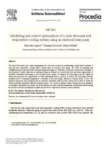
2 Baker’s Yeast Production of reduced coenzymes such as nicotinamide adenine dinucleotide (NADH) and flavin adenine dinucleotide (FADH2 ). These molecules will subsequently be used by the cell to synthesize ATP (in presence of oxygen). Moreover, the catabolism provides the carbon skeletons required for anabolism processes. Indeed, these simple molecular units will be used as precursors for synthesis of cellular components (complex organic molecules) or as material storage cells (e.g. storage carbohydrates). As all these anabolic processes require an expenditure of energy provided by ATP (endergonic reactions), they cannot take place without a parallel realization of catabolism. It should be noted that some metabolic pathways have dual anabolic and catabolic roles (amphibolic pathways), such as the Embden Meyerhof Parnas pathway and the Krebs cycle (Kristiansen, 1994; Leveau and Bouix, 1993; Waites et al., 2001). At the industrial level, the products of primary metabolism are particularly important, such as alcohols, amino acids, organic acids, enzymes and organisms themselves. Secondary metabolism generates other types of molecules used in industry, like alkaloids, antibiotics, toxins and pigments. It is interesting to note that some secondary metabolites may confer an ecological advantage, whereas others have no apparent value for producer organism. In baker’s yeast, secondary metabolites of interest are mainly storage carbohydrates. Those confer resistance to adverse conditions associated with the process of baker’s yeast production (Kristiansen, 1994; Leveau and Bouix, 1993; Waites et al., 2001). 2.2.3.1 Central Carbon Metabolism Carbon catabolism (also called central carbon metabolism) involves a series of enzymatic steps. Redox reactions are carried out to convert sugars, or other carbon compounds, in metabolic precursors and energy. In baker’s yeast, there are three main degradation pathways of carbon substrates, which are activated depending on environmental conditions (Raven et al., 2007): -
sugar respiration - complete oxidation to carbon dioxide which requires the presence of oxygen;
-
sugar fermentation - partial oxidation to ethanol which can occur in the presence or in absence of oxygen, and;
-
ethanol respiration - complete oxidation to carbon dioxide which requires the presence of oxygen.
These main degradation routes are part of various specific metabolic pathways. In this work, we will mainly focus on carbohydrate (also called glucides) metabolism and, more specifically, on metabolism of glucose and ethanol. This is because they are of central importance to the production of baker’s yeast. Indeed, there are two categories of carbohydrates: simple and
32
2.2 Saccharomyces cerevisiae: a Model Organism complex. Simple carbohydrates are composed of a single- or a double-sugar unit (monosaccharides and disaccharides, respectively). Glucose, fructose (monosaccharides) and sucrose (disaccharide: fructose + glucose) are common examples of simple carbohydrates. Complex carbohydrates, such as starch, contain at least three sugar units. Most of time, carbohydrates presenting more than one sugar unit are degraded by enzymes in single sugar units before entering the central carbon metabolism (Raven et al., 2007). Energy production from glucose is a combination of two processes: glycolysis (sequence of reactions allowing substrate-level phosphorylations3 ) and respiration (aerobic or anaerobic). Glycolysis, the Embden-Meyerhof-Parnas pathway (EMP), is a serie of ten reactions, taking place in the cytoplasmic matrix. Glycolysis consists of a reorganization of chemical bonds of glucose by several enzymes in order to generate ATP, through substrate-level phosphorylation reactions. This pathway leads to the production of two molecules of pyruvate, two molecules of ATP and the removal of four electrons from glucose bonds (reducing power4 ) per unit of glucose consumed (Kristiansen, 1994; Leveau and Bouix, 1993; Raven et al., 2007; Waites et al., 2001). The general equation of this pathway can be written as follows: Glucose + 2 ADP + 2 Pi + 2 NAD+ → 2 pyruvate + 2 ATP + 2 NADH + 2 H+
where Pi is an inorganic phosphate ion. Pyruvate produced by glycolysis occupies a central position in intermediary metabolism. Indeed, depending on the oxygen conditions, pyruvate catabolism will be directed either into the Krebs cycle (aerobic conditions) either into fermentation (anaerobic conditions). Under aerobic conditions, in order to enter the Krebs cycle, pyruvate has to be transported into the mitochondrion and be oxidized. This oxidative decarboxylation reaction converts the pyruvate into acetyl coenzyme A (acetyl CoA) and is accompanied by the reduction of NAD+ to NADH : Pyruvate + NAD+ + CoA → Acetyl CoA + CO2 + NADH + H+
Acetyl CoA is then introduced into a cycle of nine reactions : Krebs cycle, also called the TriCarboxylic Acid cycle (TCA cycle5 ). This cycle, which completes pyruvate oxidation into carbon dioxide, produces one additional ATP by substrate-level phosphorylation reaction. Moreover, this cycle allows 3 Substrate-level
phosphorylation is an ATP-generating reaction by the transfer of a phosphate group carried by an intermediate phosphorylated molecule on ADP. 4 The electrons collected in the chemical bonds are supported by NAD+ (primary electron acceptor) which is therefore reduced to NADH. 5 The term “tricarboxylic” comes from the citrate, produced in the first reaction of the cycle, which is an acid having three carboxyl groups (COO− ). Note that the TCA cycle is also called the “citrate cycle”.
33
2 Baker’s Yeast Production the capture of four extra electrons, three of them will be taken over by NAD+ and one by FADH6 . The net yield of the cycle is as follows: Acetyl CoA + 3 NAD+ + FAD + ADP→ 2 CO2 + 3 NADH + 3 H+ + FADH2 + ATP
At this stage of glucose catabolism, all molecules of ATP were produced via substrate-level phosphorylation reactions. The rest of ATP production during aerobic respiration comes from electrons captured by NADH and FADH2 . Those will be later reoxidized to allow ATP synthesis, and will then be able to be re-integrated in further metabolism. This coenzyme oxidation is carried out in mitochondrion by an Electron Transport System (ETS). This system presents a series of three membrane proteins in which electrons, carried by NADH and FADH2 , are transferred (redox reactions) to a terminal electron acceptor (oxygen). The transfer of electrons through ETS (respiratory chain) allows protons to be pumped out of mitochondrial matrix into the intermembrane space. The return of these protons to the matrix by a chemiosmotic process allows the synthesis of ATP via ATP synthase7 (Kristiansen, 1994; Leveau and Bouix, 1993; Raven et al., 2007; Waites et al., 2001). Under anaerobic conditions, pyruvate is directed into fermentation. As oxygen is not available as a terminal electron acceptor, an alternative mechanism has to be used for regeneration of the coenzymes (NADH and FADH2 ), reduced during the oxidation of glucose to pyruvate (glycolysis). Fermentation is achieved by transferring electrons collected during glycolysis to an organic molecule derived from pyruvate; acetaldehyde. Acetaldehyde will be further reduced to ethanol in order to generate NAD+ (Kristiansen, 1994; Leveau and Bouix, 1993; Raven et al., 2007; Waites et al., 2001). Figure 2.1 presents a schematic overview of all the afore mentioned metabolic reactions linked to the central carbon metabolism. As underlined above, aerobic respiration and fermentation are regulated by environmental conditions, which include oxygen availability and sugar concentration in the medium. The Crabtree and the Pasteur effects are the two major phenomena of energy metabolism regulation (glucose metabolism) depending on culture conditions. Under aerobic conditions, many organisms exhibit a slower rate of sugar catabolism via glycolysis than under anaerobic conditions. In fact, glucose respiration is favored because fewer carbon units are required to obtain same quantity of ATP. Indeed, aerobic respiration and associated oxidative phosphorylation allows a considerably higher energy recovery than fermentation. 6 Similar
to NAD+ , the FADH is a carrier-energy coenzyme which is reduced to FADH2 . Its specificity is that it is exclusively located in the mitochondria. 7 ATP synthase uses the energy stored as a proton gradient on either side of the inner membrane of the mitochondrion to catalyze the ATP synthesis from ADP and Pi .
34
2.2 Saccharomyces cerevisiae: a Model Organism
Figure 2.1: Central Carbon Metabolism (Raven et al., 2007).
This inhibition of fermentation by the presence of oxygen is a regulatory phenomenon referred to as the Pasteur effect, which is apparent only at low sugar concentration (concentration value depends of yeast strain) (Leveau and Bouix, 1993; Waites et al., 2001). Several yeasts exhibit another regulatory phenomenon: the Crabtree effect. The Crabtree effect consists of an inhibition of aerobic catabolic pathway of respiration and promotion of ethanol production even in the presence of oxygen (fermentative pathway). The proposed explanation is that an excess of glucose causes a saturation of the respiratory capacity of Crabtree-positive organism and thus causes repression of several respiratory pathways (Leveau and Bouix, 1993; Waites et al., 2001). These two effects are combined in the concept known as“overflow metabolism”. Although not fully understood, this phenomenon is related to the existence of a critical rate of sugar uptake (strain-dependent). This concept explains why we can observe ethanol production under aerobic conditions by saturation of respiration (excess of sugars input due to high sugar concentrations). Indeed, below a critical rate of sugar uptake, all sugar assimilated by yeast is fully oxidized to CO2 (glycolysis + TCA cycle). However, when a critical concentration of glucose is reached, sugar is metabolized faster than the critical rate. The surplus of pyruvate that cannot be oxidized aerobically is then reduced to ethanol instead of entering the TCA cycle (Sonnleitner and K¨appeli, 1986).
35
2 Baker’s Yeast Production However, fermentation is very wasteful in terms of recovery of potential energy from glucose. Indeed, to produce the same amount of energy (molecules of ATP per glucose consumed), yeasts will consume ten times more sugar by fermentative route than by respiration. Therefore, yeasts will preferentially degrade sugar by respiration rather than by fermentation as long as possible. 2.2.3.2 Central Nitrogen Metabolism As stated above, nitrogen, as a main component of proteins and nucleic acids, is an essential nutrient both for microorganism growth, and for the cellular metabolism activation. Indeed, nitrogen plays a central role as intermediate between the catabolic and anabolic pathways (Magasanik and Kaiser, 2002; ter Schure et al., 2000). Saccharomyces cerevisiae is able to assimilate a wide variety (almost 30 distinct) of nitrogen sources. Uptake takes place through more or less specific permeases expressed following the nature and the concentration of nitrogen sources8 . These nitrogen-containing compounds are defined as good or poor nitrogen sources based on their ability to support cell growth. Good nitrogen sources such as ammonia, glutamine and asparagine lead to a higher growth rate than with poor nitrogen sources, such as urea and proline. For example, growth rate on ammonium sulfate, which qualifies as a good source, leads to similar generation time (2 h) than growth on glutamate and glutamine (2.15 h et 2.05 h respectively) which are often defined as the “preferred” nitrogen sources whereas urea leads to 3.35 h of time generation. Therefore, if more than one nitrogen source is available in a culture medium, S. cerevisiae will promote the uptake of nitrogen-containing compounds enabling the best growth by a mechanism called Nitrogen Catabolite Repression (NCR) (Godard et al., 2007; Magasanik and Kaiser, 2002; ter Schure et al., 2000; van Riel et al., 1998). Once inside the cell, the nitrogen source needs to be degraded into useful building blocks (N H2 group donor compounds) for biosynthesis reactions via specific metabolic pathways. Central Nitrogen Metabolism (CNM) is directly linked to the TriCarboxylic Acid cycle through α-ketoglutarate, provided by 8 The
absorption of nitrogenous compounds involves permease families which are specific to the nature of the nitrogen source, such as specific carriers for amino acids. A good example of the expression modulation of these carrier families - depending on the concentration - can be given with the ammonium permease family (Mep transporters). Three permeases (Mep1p, Mep2p and Mep3p) are involved in ammonia uptake. They are only expressed at low nitrogen concentration and each of them presents a specific affinity for N H4+ . Indeed, they can be ordered by decreasing constant affinity as follows: Mep1p (Km = 5 − 10M ), Mep2p (Km = 1 − 2M ) and Mep3 (Km = 1.4 − 2.1mM ). Note that growth on ammonium sources at concentrations higher than 20 mM (0.36 g/L of N H4+ ) does not require any of the Mep permeases (ter Schure et al., 2000).
36
2.2 Saccharomyces cerevisiae: a Model Organism
Figure 2.2: Interconversion of α-ketoglutarate, ammonia, glutamate and glutamine in the Central Nitrogen Metabolism (ter Schure et al., 2000).
the central carbon metabolism, to produce glutamate and glutamine. Glutamate and glutamine are the two major nitrogen donors in biosynthesis reactions (respectively 85% and 15% of the total cellular nitrogen). Therefore, they have both a central position in the CNM (Magasanik and Kaiser, 2002; ter Schure et al., 2000; van Riel et al., 1998). Figure 2.2 represents the interconversion between ammonia, glutamine and glutamate where ammonia is directly used as the amine group donor. When cells have an abundant source of ammonia, α-ketoglutarate (TCA cycle intermediate) is directly converted into glutamate by the NADPH-dependent glutamate dehydrogenase (NADPH-GDH). The inverse reaction is also possible thanks to the NADH-dependent glutamate dehydrogenase (NADH-GDH): + α-ketoglutarate + NH+ ↔ Glutamate + NAD(P)+ 4 + NAD(P)H + H
Glutamate can then be converted into glutamine by an enzyme called glutamine synthetase (GS): Glutamate + NH+ 4 + ATP → Glutamine + ADP + Pi
The inverse reaction (glutamine into glutamate) is catalyzed by an enzyme called glutamate synthase (GOGAT): Glutamine + α-ketoglutarate + NADH + H+ → 2 Glutamate + NAD+
2.2.3.3 Storage Carbohydrates Metabolism As mentioned earlier, some metabolites may confer ecological benefits on the cells, e.g. by allowing rapid adaptation to environmental changing conditions. For baker’s yeast production, culture conditions are often optimized
37
2 Baker’s Yeast Production to obtain a high amount of storage carbohydrates. Indeed, these carbohydrates are energy storage compounds. Note that baker’s yeast is usually cultured in excess nutrient conditions. This nutrient excess can be stored into cells and will be used during potential starvation periods (Aboka et al., 2009; Attfield, 1997; Waites et al., 2001). The two main glucose storage units are glycogen (polysaccharide) and trehalose (disaccharide). These may confer qualitative properties of industrial interest in Saccharomyces cerevisiae. Glycogen is a big polysaccharide of linear α-(1,4)-glucosyl chains branched with α-(1,6)-linkages. Trehalose is a disaccharide composed of two α-(1,1)-linked glucose units. When required, these polymeric reserves are hydrolysed by phosphorylases, liberating glucose-1-phosphate. This last one can directly enter into catabolism to act as a carbon and energy source. Hence, much attention during the last few decades has been given to characterizing the biochemical and molecular organisation of glycogen and trehalose metabolism, providing important new insights into the function of these glucose stores in yeast (Aboka et al., 2009; Attfield, 1997; Fran¸cois, 2001; Guillou et al., 2004; Hazelwood et al., 2009; Jørgensen et al., 2002; Lillie and Pringle, 1980; Parrou et al., 1999; Sillje et al., 1999; van Dijck et al., 1995; Waites et al., 2001). We will not make a specific explanation of all the metabolic pathways that lead to the synthesis and the degradation of these compounds. To this end, the reader can refer to the review about regulation of the activity of the enzymes involved in the pathways of synthesis and degradation of trehalose as well as on the transcriptional control of the encoding genes (Fran¸cois and Parrou, 2001). This work will focus on the importance of these carbohydrates as carbon and energy reserves in the “stress response” (more precisely during nutrient starvation) and on their potential interconnections with central metabolism of carbon and nitrogen. Indeed, many researchers have studied the influence of these carbohydrates on physiological and metabolic activity in yeast cells. It has been suggested that these metabolites are of crucial importance for adaptation to aerobic conditions, during the germination of spores, upon entry into stationary phase as well as in the recovery of metabolic activities of cells emerging from the stationary phase and during nutrient starvation conditions. Glycogen fits quite well with the concept of metabolite storage of carbon and energy: it accumulates mainly in conditions of nutrient excess (e.g. during fermentation) and is mainly mobilized during the stationary phase when all sources of nutrients have been exhausted. However, trehalose does not seem to agree with this concept. Indeed, trehalose accumulation is principally known to be induced under three circumstances: reduced growth rate, growth on nonfermentable carbon sources (as ethanol) and harmful environmental conditions, such as high temperature, osmotic shocks and nutrient limitation. Moreover, trehalose is not necessarily mobilized in stress conditions such as nutrient
38
2.3 Industrial Production Process starvation (Aboka et al., 2009; Attfield, 1997; Fran¸cois, 2001; Guillou et al., 2004; Hazelwood et al., 2009; Jørgensen et al., 2002; Lillie and Pringle, 1980; Parrou et al., 1999; Sillje et al., 1999; van Dijck et al., 1995; Waites et al., 2001). Many studies suggest that trehalose plays an important role in the stress response of yeast cells. Indeed, these studies have shown that only 2-3% of dry mass in intracellular trehalose improves cell viability and could enhance the physiological activity of dried yeasts produced in industrial fermentations. Moreover, trehalose seems to improve the industrial aspects related to the quality of baker’s yeast such as leavening capacity in dough and tolerance to freezing and dehydration (drying). In particular, its ability to maintain the structural integrity of the cellular cytoplasm (protection from autolysis) under harmful environmental conditions has led scientists to refer trehalose as a “stress protectant”. It is interesting to note that the metabolism of trehalose has a significant “turnover” (simultaneous synthesis and degradation). It has been hypothesized that this feature, although it represents a considerable loss of energy, would ensure the continuous synthesis of enzymes required for the mobilization of storage carbohydrates during any sudden change in environmental conditions (Aboka et al., 2009; Attfield, 1997; Ertugay, 1997; Fran¸cois, 2001; Guillou et al., 2004; Hazelwood, 2009; Jørgensen et al., 2002; Lillie and Pringle, 1980; Parrou et al. et al., 1999; Sillje et al., 1999; van Dijck et al., 1995).
Section 2.2 clearly underlines that microorganisms are remarkably adaptable to their environment through cell metabolism. This complex metabolic system provides a connection between external stimuli and growth. Therefore, the study of metabolic adaptation mechanisms is of particular interest in industrial microbiology. Indeed, knowledge of metabolism specificities allows manipulation of metabolic pathways in order to suit the industrial process requirements, e.g. by forcing the production of specific metabolites. This can be achieved by initial strain selection and development (mainly by genetic modifications) or optimization of fermentation conditions. In the case of this work, only the last topic will be studied.
2.3 Industrial Production Process Until the early 19th century, the industrial production of baker’s yeast was performed with yeasts issued from beer fermentation. The baking industry only really emerged after new strains of yeast were found, and new cultures conditions implemented. Indeed, brewer’s yeast strains were not adequate for optimal bread production. In addition, the model of production by anaerobic
39
2 Baker’s Yeast Production fermentation of malted barley grains, based on the beer production process, induced low growth yield due to the high ethanol production (Kristiansen, 1994; Leveau and Bouix, 1993; Pomerleau, 1990; Waites et al., 2001). Hence, two major improvements of production conditions have been introduced in the production process of baker’s yeast: -
the aeration of the culture medium. The supply of oxygen reduced ethanol production by ensuring aerobic culture conditions;
-
the development of the fed-batch process. Initially called “Zulauf” process, this technique, developed by the Germans in 1930, consists of a gradual supply of substrates to the culture. This allows the control of the substrate feeding throughout the culture, e.g. by maintaining a sufficiently low concentration of sugars in the culture medium to avoid the production of ethanol (Crabtree effect).
Quality and quantity will always be the two fundamental objectives in any economical optimization of industrial production: achieve a product of good quality in large quantities within a given time period. However, these two objectives are often opposed. Thus, manufacturers must currently deal with a compromise between the quality of the product and productivity of the production process. This is the case for baker’s yeast production. Indeed, the ideal operating conditions to ensure good baking characteristics are not optimal for ensuring a maximum yeast production (Attfield, 1997; Enfors et al., 1993; Kristiansen, 1994; Randez-Gil et al., 2013). Factors influencing the qualitative and quantitative aspects of the yeast production, as well as the types of compromise necessary to optimize the latter, will be developed in this section. To this end, Section 2.3.1 will present the qualitative characteristics of baker’s yeast as a final product. This section will highlight the importance of managing the various stages of production (pretreatment, yeast production, recovery, treatment, and storage) to ensure the quality of the produced yeast. Section 2.3.2 will present the aspects concerning appropriate choice of the raw materials used for production. Indeed, culture medium composition is closely related to the acquisition of the qualitative characteristics but is also the main cost factor on industrial production. The description of the bioreactor specificities for the production of baker’s yeast (Section 2.3.3) will allow the reader to better understand how the control of operating conditions process (pH, aeration, temperature, etc.) can lead to an efficient use of available substrates. To close this chapter, the Section 2.3.4 will present an overview of the production process of baker’s yeast as performed in an industrial context today .
40
2.3 Industrial Production Process
2.3.1 Baking Characteristics Although quality may be defined in many ways, the two main qualitative criteria of commercial baker’s yeast are the activity (effectiveness of the production of carbon dioxide) and the stability (capacity to maintain the activity over the time). These properties are influenced by the yeast strain, the production process and the choice of raw materials (Attfield, 1997; Randez-Gil et al., 2013; Kristiansen, 1994). The primary role of baker’s yeast in the bread-making process is to efficiently leaven bread dough. This property is related to the fermentative activity of yeast: its ability to ferment sugar in the dough vigorously and quickly (high glycolytic activity) that is also called the “gassing power” (CO2 production rate). In addition, there are now a variety of specific baking processes, such as those for sweet and frozen dough, in which yeast cells are exposed to many environmental stresses. To cope with these conditions, yeast cells must have significant adaptation capacity which can be called stress-tolerance properties. Thus, in sweet dough, yeast should have high osmotolerance, i.e. the ability to function in the presence of high levels of sugars (or salts) within the dough (Attfield, 1997; Najafpour, 2006; Randez-Gil et al., 2013; Kristiansen, 1994; Waites et al., 2001). Yeast activity must be preserved in all stages of the production process from the yeast production to bread making (downstream processing, including washing, dewatering, and drying). This property, called the stability of yeast, is strongly correlated with the ability of yeast to adapt quickly to changes in its environment (stress tolerance properties mentioned above). Indeed, in order to be directly active when introduced into the dough, the yeast must be able to keep some intrinsic properties operational upon entry into the stationary phase, at the end of the production process. These properties of stress tolerance, such as osmotolerance, thermal and desiccation tolerances, are strongly correlated with the accumulation of heat-shock proteins and small protective molecules, such as trehalose, at the entry into stationary phase. Indeed, trehalose has the ability to replace the shell of water around macromolecules, which makes it an excellent antioxidant that can, for example, mitigate some damaging effects during drying. Like the freezing-thawing process, drying is a “multiple-nature stress” which combines high temperature and dehydration. These stresses (heat and desiccation) generate macromolecular damages, especially to the cell membrane and proteins. Therefore, culture media and the process conditions implemented during production have traditionally been optimized to ensure that high levels of protective molecules are synthesized (Attfield, 1997; Najafpour, 2006; Randez-Gil et al., 2013; Kristiansen, 1994). Regarding the culture conditions, it was demonstrated that under aerobic conditions yeasts have greater stability than under anaerobic conditions.
41
2 Baker’s Yeast Production These aerobic conditions lead to the highest growth rate possible for yeast but result also in a low protein content and high levels of carbohydrates. Those factors are responsible for stability improvement. This cell composition is also provided by stopping the ammonia and molasses feeds before the end of the process. Indeed, this allows the yeast to assimilate any remaining sources in the culture medium substrates and to store those nutrients. Particularly, yeasts store carbohydrates which are used as energy source during storage of the yeast as finished product. However, it is important to note that the acquisition of a good activity (high fermentation performance) requires sufficient levels of proteins in cells, contrary to the stability acquisition. Hence, production of baker’s yeast must ensure an appropriate balance between a high protein and high carbohydrate contents. Furthermore, it is important to ensure that all yeasts are in a similar physiological state at the end of production process so as to obtain a homogeneous final product. The acquisition of this homogeneity is another reason to stop the supply of molasses which allows yeast to mature (cessation of reproduction cycle). These observations support the importance of the physiological conditioning by culture environment control during cultures as a way to optimize baker’s yeast production performance in terms of both quality and quantity (Attfield, 1997; Najafpour, 2006; Randez-Gil et al., 2013; Kristiansen, 1994; Waites et al., 2001).
2.3.2 Medium Composition Baker’s yeast is produced aerobically in a medium containing principally carbon, nitrogen, sulphur and phosphorus sources and additional salts and vitamins (Table 2.3). Table 2.3: Example of medium composition for baker’s yeast production based on average yeast composition (Kristiansen, 1994). Ingredient for 1 m3 of fermentation medium Molasses Ammonia KH2 PO4 MgSO4 Biotin Ca pantothenate Inositol
198 kg 10.5 kg 8.75 kg 0.75 kg 50 mg 10 mg 10 g
While glucose is the preferred carbon source of yeast, it is rarely used on an industrial scale due to its high cost. Instead of glucose, molasses are used as a
42
2.3 Industrial Production Process carbon source for yeast production. This byproduct of the sugar production (sucrose extraction) from cane or beets is obtained after crystallization of the plant extract. It presents itself as a dark viscous syrup containing carbohydrates, nitrogenous compounds, salts and vitamins. As a major constituent of the culture medium, the composition of the molasses plays a crucial role in the baker’s yeast production performance and is often a real problem for manufacturers wishing to produce a yeast with a constant quality. A typical molasses composition is presented in Table 2.4. However, it is important to underline that molasses composition is influenced by many factors and nutrients content can vary depending on the production lot which molasses is derived (vegetable source, geographical and climatic conditions, refinery technology used, etc.) (Kristiansen, 1994; Waites et al., 2001). Table 2.4: Typical molasses composition (Kristiansen, 1994). Element
Concentration (%w/v)
Water Sucrose Glucose Fructose Other reducing substances Other carbohydrates Nitrogen Compounds Non-nitrogen acids Wax, sterol, phospholipids
17-25 30-40 4-9 5-12 1-5 2-5 2-6 2-8 0.1-1
Molasses is principally composed of carbohydrates (40-60% w/v) which can be used as carbon source. It should be noted that the sucrose contained in molasses cannot directly be assimilated by yeast: it has to be hydrolyzed “extracellularly” (by a periplasmic invertase) into glucose and fructose units which can then be transported into the cells. Molasses also contain between 2-6% (w/v) of nitrogenous substances. However, only a very small portion (approximately 0.2%) can really be assimilated by the yeast. Hence, an additional nitrogen source must be supplied to the culture. On industrial scale, this source is generally provided in the form of ammonia, which also serves as a pH regulator (note that ammonium salts or urea may also be used as nitrogen source). As molasses generally does not contain sufficient amounts of phosphorus to ensure optimal growth conditions, culture is often supplemented with additional source such as ortho-phosphoric acid (also used for pH regulation) or other appropriate forms of phosphate (Kristiansen, 1994). In addition to nitrogen and phosphorus, mineral salts (source of potassium, magnesium, calcium and sulfur) and vitamins must often be added to the
43
2 Baker’s Yeast Production culture medium. Indeed, these essential elements are often present in low quantities in the molasses and depending on the strain of yeast used, the nutritional requirements for cell growth can vary substantially (Kristiansen, 1994; Waites et al., 2001).
2.3.3 Bioreactor Description: Monitoring and Control A bioreactor is a vessel in which the microorganisms are cultured with controlled environmental conditions. These tanks were initially called “fermenters” but the term “bioreactor” was rapidly preferred to emphasize the potential aerobic nature of culture conditions. Their volume capacity can be in the range 2-100 liters for pilot laboratory scale and up to 100 m3 in the case of bioreactors used at the industrial production scale. There are many different types of bioreactors: each of them allowing some adaptations to the specific needs of the cultured microorganisms and application context; e.g. the fluidized bed bioreactor is often used for waste treatment and the bubble column bioreactor is useful for algae cultures. The most common form is the simple stirred tank bioreactor with a central rotary axis on which agitators are disposed in order to ensure a good mixing of the culture medium (Alford, 2006; Najafpour, 2006; Renard, 2006). This kind of bioreactor can be operated in different modes by acting on the flow rates of feeding medium addition, noted F in and outlet of culture medium, noted F out : -
Batch mode: all substrates are added at the beginning of culture and nothing is added (F in = 0) or removed (F out = 0) from the bioreactor. The volume of culture medium remains constant and the cells grow until the exhaustion of substrates. This type of operating mode is therefore entirely dependent on the concentrations (in substrates and microorganisms) initially present in the bioreactor. Hence, problems related to excessive dilution of the inoculum concentrations (quantity of cells used to start the culture) or growth inhibiting concentrations of substrates are often encountered in batch mode and can lead to low efficiency of the process;
-
Fed-batch mode: the bioreactor is fed continuously in a culture medium (F in != 0), while the outflow remains nul (F out = 0). The culture volume increases continuously and the cells grow until the achievement of the maximum volume capacity of the bioreactor. The feeding flow rate of substrates (F in (t)) determines mainly the cell growth rate and allows also to maintain the concentrations of substrates in the culture medium at thresholds preventing potential inhibitory effects on the growth (e.g.
44
2.3 Industrial Production Process Crabtree effect in yeasts). In addition, this operating condition enables to start the process with low volumes. This promotes a rapid growth start since the initial cell concentration can be higher for a same quantity of cells. The fed-batch mode often leads to higher yields of the process and is the most popular mode used in industry for these pre-mentioned reasons; -
Continuous-mode: the bioreactor is fed continuously (F in != 0) and the culture medium is continuously removed (F out != 0). If feeding and outlet rates are equal, volume of the culture medium can be considered constant and cell growth can be maintained at a steady state. This type of operating mode is very useful for metabolic studies of different organisms as the cells can be maintained in a specific physiological state throughout the culture time. Therefore, the influence of environmental factors (e.g. pH, tempreature, etc.) on cell growth can be easily studied.
The advantage of cultures in bioreactor is the ability to control growth environmental conditions. Indeed, cell growth is driven by complex interactions between chemical and physical environmental conditions and cell metabolic activities. Hence, good management of these environmental conditions can ensure reproducibility of production processes but also ensure optimal conditions for the considered process. Therefore, sufficient information about the bioreactor operating conditions and their influence on cultured organisms is needed. To this end, the variables characterizing the operating conditions can be measured on-line and thereby become a means of action to direct the operation of the bioprocess (Alford, 2006; Harms, 2002; Najafpour, 2006). The key physico-chemical parameters involved depend largely on the bioreactor type, its mode of operation and the microorganisms. Standard instrumentation of bioreactors in industrial processes is used for the measurement of temperature, pressure, pH, aeration, stirring rate, foam and dissolved oxygen concentration. Some bioreactors are also connected to an analyzer which provides the on-line composition of the exhaust gases (oxygen and carbon dioxide contents) (Alford, 2006; Harms, 2002; Najafpour, 2006). The basic principle of control is to keep some of these operating parameters at a desired threshold value within the bioreactor. The data from the instrumentation measurements (probes) are recorded on a computer having a control system. The objective of this control system (feedback loop) is to maintain the difference between the signals measured by the sensors and desired values (set by the operator) to a minimum level. In addition, experimental data collected can be used to perform some appropriate calculations, allowing, for example, to have real-time information on cell population and product yields, transfer rates of oxygen and carbon dioxide, uptake rate of nutrients, etc. (Alford, 2006; Harms, 2002; Komives and Parker, 2003; Najafpour, 2006).
45
2 Baker’s Yeast Production Figure 2.3 shows a schematic representation of the bioreactor used in this work: a BIOSTAT C-DCU3 (Sartorius B. Braun International) of 20L. The digital control unit (bioreactor memory linked to the sensory system) of the bioreactor is connected to an interface called MFCS/win (Sartorius B. Braun International) in order to record all the data on a computer during the experiments.
Figure 2.3: Schematic representation of a bioreactor.
2.3.4 Process Operating Conditions In the context of baker’s yeast production on an industrial scale, the production target is the yeast itself. To this end, the production bioreactors are operated in fed-batch mode. Contrarily to the batch mode, the fed-batch operation enables to maintain low sugar concentrations in the medium. High sugar concentrations would result in a significant production of ethanol that will inhibit yeast growth due to overflow metabolism. In addition, as industrial bioreactors possess a limited gas transfer capacity, the management of growth rate and composition of the culture medium via the modulation of the feeding flow rate of substrates allows manufacturers to influence the oxygen demand. Indeed, high concentrations of sugars and cell population decrease gas transfer capacity in the culture medium due to the high viscos-
46
2.3 Industrial Production Process ity of this last. It requires increased aeration9 to ensure sufficient oxygen supply in the overall culture medium (Kristiansen, 1994; Waites et al., 2001). The evolution of the process is almost entirely governed by feeding profile over the time in carbon (molasses) and nitrogen (ammonia) sources. This profile, often defined by trial and error at the stage of the process development, has generally a similar pattern in all baker’s yeast production industries. Indeed, it generally follows a growing curve until a certain cell population concentration has been reached. It is then kept constant, and finally stopped at the end of culture. It is important to note that this feeding profile is generally fully defined with respect to the carbon source. The supply of nitrogen is determined a posteriori as a function of the sugar feeding profile by establishing a C:N ratio, which needs to be maintained constant during culture (Enfors et al., 1990; Kristiansen, 1994; Waites et al., 2001). Generally, the first phase of culture is defined according to the principle of exponential growth: the carbon source feed rate increases at the same speed as the cell population increases10 . In practice, this profile is also defined to obtain a little production of ethanol, in the range of a few grams per liter (below the inhibitory concentration), while avoiding the accumulation of sugar in the medium (potential loss of yield). Produced ethanol is then consumed by the yeast when the flow rate is held constant. This constant feed phase can be extended to permit the consumption of the produced ethanol, which also allows to achieve higher cell concentrations. It can be noted that this ethanol production enhances the process production (quantity of yeast produced for a given culture time). Indeed, if the feeding time profile is engineered in order to maintain growth rate at or below the threshold of respiratory capacity (during which no ethanol is formed), growth rate would be greater but the production of yeast would be lower. Hence, the feed profile selection is often the result of optimization and the choice between a compromise: high yield / low production or low yield / high production (Enfors et al., 1990; Kristiansen, 1994; Pham et al., 1998; Waites et al., 2001). The feeding is stopped at about 50-60 g dry cells per liter (obtained after 15 hours with an inoculum size of 10% (v/v)). The termination of a baker’s yeast process is a critical procedure that aims at maturing the yeast to give it suitable qualities such as activity (the rate of CO2 production in the dough), storage stability (the rate by which the gassing power declines during the storing) and stress resistance. Some maturation methods include the cessation of the nitrogen and subsequent stepdown of the molasses feeding in order to force cells to terminate their cell cycle (cessation of budding) and to accumulate intracellular carbohydrates. During this last phase, cell com9 The
transfer rate can also be increased by a higher agitation. However, there is a maximum value of the stirring speed that should not be exceeded as this may cause damage to cells. 10 The specific growth rate during the exponential phase is approximately equal to 0.25 h
47
2 Baker’s Yeast Production position in proteins and carbohydrates changes considerably. The trehalose concentration increases during the maturation phase and is considered to be very important for the storage quality11 . Protein content, often associated with enzyme activities of the yeast, is also controlled by the feed profiles and nitrogen-to-sugar ratio during the process. The positive correlation between high protein concentration and high activity, together with the negative correlation between protein concentration and storage stability, is one mean by which the manufacturer can adjust the desired properties of the product (Kristiansen, 1994). The operating temperature of baker’s yeast fermentation is 30°C. This is a compromise between the temperature at which the highest attainable cell population yield on sugar is reached (28,5°C) and temperature at which the maximum growth rate is reached (32°C). Contrarily, the pH value is changed during the process ; it is raised from 4 to approximately 5.5. The pH profile of the fermentation is also the result of a compromise. Due to the fact that baker’s yeast grows faster than bacteria at low pH values, it is advantageous to operate at low pH values in order to avoid contamination, especially at the low cell population concentrations of the preparing stages. However, it is within the pH range of 5 to 5.5 that growth reaches its maximum. Hence, the compromise is a pH value around 4 for most of the process with a raise to 5.5 towards the end. The higher value is also due to the quality requirements ; at low pH values pigments are more easily absorbed by the yeast, and the concentration of ammonia which colours the yeast is higher. To achieve a light-coloured product, pH is increased preferably by terminating the ammonia feed. Indeed, the ammonia consumption results in a pH decrease : one proton is liberated for each N H4+ ion that is consumed (Kristiansen, 1994).
11 About
1% of the cell content in glycogen and trehalose is degraded per day during storage at 4 °C.
48
3 Modelling of Bioprocesses 3.1 Introduction A process is defined, in the dictionary, as a method used to achieve a certain result by performing a specific function. A biological process, or bioprocess, is a method that uses living organisms or cellular components to transform raw materials into a desired product. It can also be defined as a system comprising a set of elements (inputs, outputs and states1 ) which interact in accordance with certain rules in order to ensure a given production. A mathematical model is a set of “mathematical relations linking essential variables of a system” which allow a simplified representation of the structure and the behavior of this system. This representation can be more or less complex depending on the modelling objectives. Indeed, the aim of the mathematical description of a system can be purely “ontological” or more “utilitarian” (as in this work). An “ontological” model is developed in order to provide an explanatory description of some aspects of the system’s general behavior. Therefore, a “good ontological” model must be as specific as possible in describing mechanisms of the system under study. In doing so, such models have often a large number of mathematical relations linking the numerous variables characterizing the system and are associated with a large number of parameters (high structural complexity). Unlike “ontological” models, an “utilitarian” model is developed in order to provide a tool, e.g. for process optimization (improvement of some system properties), control (maintenance of the system in a specific behavioral state), design (conception of a process plant exploiting the system behavior). Thus, a “good model” with “utilitarian” purposes must have a smallest as possible structural complexity and a large range of validity - in other words, a significant ability to predict the system behavior as accurately as possible in a large range of operation conditions. These two criteria are essential for using the model as a tool for process optimization, control or design. Hence, regardless of the studied system, it is necessary to objectively respond to the question “for what purposes the model will be used?” in order to develop an appropriate model for the achievement of modelling goals. 1 The
inputs are all signals that act on the system (commands and disturbances) and induce an external response (output variations) by a change in the state of the system (system memory).
49
3 Modelling of Bioprocesses After a clear definition of the modelling objectives, the development of a model is based on the choice of three key components: an experimental field, a model structure and an identification method (mainly based on the choice of an identification criterion). To this end, a basic amount of a priori knowledge of the studied system is needed. This knowledge will allow the definition of the general properties of the model and, in doing so, the selection of a family of candidate model structures. These properties depend on the specific characteristics of the studied process such as the linearity or the nonlinearity of the behavior of the subject, the parameter properties (constant or evolving), the manner of taking into account the time scale of the system, etc. Once these properties are defined, an essential modelling step is experimentation. This allows the generation of informative data (experimental field) that will be used to attribute values to the different parameters introduced in the model by using a parameter estimation procedure. The existing parameter estimation methods are numerous and depend on the choice of an identification criterion (cost function). The role of the identification criterion is to help one choose objectively the best model from the family of candidate models. It defines a distance between the data generated by a candidate model (predicted model outputs) and those achieved during the experimentation. Hence, the parametric estimation consists of the optimization of the selected cost function in such a manner that this distance will be the smallest possible. The last step of the modelling procedure is the validation of the constructed model. Validation verifies that the model is representative of the system behavior while meeting the objectives for which it was developed. This decision-making process is far from linear and the interdependence between these different components leads the modeler to cast doubt on these choices at each stage of the model’s development. In this chapter, the main theoretical aspects related to the development of a model at the macroscopic scale will be discussed. After a brief introduction on the benefits of the use of models in the development of industrial bioprocesses, the theory linked to the structural model properties and mathematical aspects underlying their development will be presented in Section 3.2. Section 3.3 will present the theoretical aspects related to the parametric estimation step (experimental field, identification criteria and algorithms). Tests to assess the quality of the developed model and its final validation will be presented in Section 3.4. To conclude this chapter, the model of Sonnleitner and K¨ appeli (1986) will be presented in Section 3.5.
50
3.2 Simulation and Modelling
3.2 Simulation and Modelling: a Tool for the Development of Industrial Bioprocesses In an industrial context, the main purpose of process modelling is most often an economical optimization of production: the goal is to identify the system properties that can be used to define an optimal behavior in terms of improving the productivity (and/or yield) of the process. However, the definition of these optimal operation conditions is often achieved with a trial-and-error method at the industrial scale of process development. This long and tedious strategy leads to a heuristic solution mainly based on the empiric knowledge of the process system. Moreover, it is quite impossible to ensure that this solution leads to the achievement of an optimal productivity (and/or yield). In this context, mathematical modelling provides a useful tool for searching for an optimal solution. Indeed, thanks to a model with good prediction capacity, it is possible to test many experimental conditions, even outside of the usual functioning range, where the realization of real-life experiments would be hard to carry out for practical, economical or security reasons, which is often the case in biotechnology. Moreover, a mathematical model of a process, which covers the description of the overall behavior that a system can exhibit, allows the precise definition of every state variable that may significantly influence the process (Dochain, 2008). Hence, this model-based approach can be viewed as a first step of the economical optimization strategy as this powerful tool represents the potential forgains of time and money by allowing objective choices for the development and the improvement of numerous industrial processes.
3.2.1 What Kind of Models? As cited before, the modelling of a system could present different levels of complexity depending on the modelling goals. Indeed, a model whose objective is to describe as accurately as possible the mechanisms underlying the operation of a process will certainly have a greater structural complexity than a model developed for purposes of optimization of this process. Furthermore, it is important to note that the dynamics related to the operation of the process can themselves vary in complexity. Obviously, it is much easier to model the operation of a flushing toilet than to model the operation of a combustion engine. Hence, a part of the structural complexity of a model will also mirror the complexity of the system being studied. In biology, modelling is a very hard task due to the inherent complexity of cell metabolism involved in bioprocesses, such as cultures in a bioreactor. Indeed,
51
3 Modelling of Bioprocesses cell metabolism is a network of many hundreds of reactions that take place between multitudes of components and interact through intern regulation mechanisms. The whole network forms a nonlinear dynamic system. Over the past decades, the advances in the mathematical modelling of such complex systems have led to the possibility of describing and quantifying, at the microscopic scale, all these reactions in a limited and very specific system (“ontologic” models). These complex models, known as structured models, are very useful for descriptive purposes as they aim at studying very specific metabolic mechanisms (Rizzi et al., 1997). However, these models are very difficult to handle for utilitarian purposes as they have a huge structural complexity and a small range of validity (in opposition to the “good utilitarian model” definition given above). Indeed, the optimization and the control of this kind of “biosystem” are almost impossible if a more simplified description is not taken into account. In this context, some assumptions need to be made in order to make modelling possible. These assumptions allow some simplifications of the representation of complex systems while guaranteeing that the general behavior is always described. First of all, it is important to realize that the modelling of a bioprocess always includes at least two systems: the bioreactor and the cell population. These systems overlap. Indeed, the cell population is the content of the bioreactor where each cell can be represented as a small system within the overall system. The behavior of the bioreactor and the cell population systems present very different properties such as kinetics, transport, and dynamics time scales. Moreover, the cell population presents fluctuations in the age distribution leading to a different specific state of the yeast life cycle for each cell at any time during the bioprocess. To overcome this problem, cells can be considered as homogeneous catalysers: this is the assumption of non-segregation of the cell population. Furthermore, as each cell has clearly defined boundaries towards the rest of the bioreactor and as all cells present the same behavioral properties (non-segregation assumption), another modelling assumption is to globalize the overall population in only one variable, which is commonly called biomass (Bogaerts, 1999; Walter and Pronzato, 1997). Therefore, these approximations allow one to consider only one system: the bioreactor in which the reactions “directly” take place. Finally, the biomass and the other influencing factors of the bioprocess, such as the substrates, become macroscopic components (expressed in terms of external concentrations) that are assumed to be equally distributed throughout the bioreactor system. These assumptions are the basic concept of the unstructured and unsegregated models with ideal mixing. The emphasis of model description has been put on simplicity and only takes into account the evolution of the macroscopic components of interest. Contrary to structured and segregated ones, these kinds of macroscopic models have considerably more simple struc-
52
3.2 Simulation and Modelling ture and allows generally a good description of the system in a large range of conditions (Bogaerts, 1999; Walter and Pronzato, 1997). For a review of the mathematical models for growth and product formation of the most important microorganisms, we refer the reader to the relevant review of Nielsen and Villadsen (1992). It is important to note that there exist techniques for reducing metabolic models at the macroscopic scale (Haag et al, 2005; Provost and Bastin, 2004; Zamorano et al., 2013) which relates the biomass and the extracellular components. However, until now, there are still open problems in the way to handle the reduction procedure: the definition of different metabolic networks for different phases of the culture, the switching from one phase to the other, the link between the unstructured and unsegregated biomass with the intracellular fluxes, the use of macroscopic models for the global consumption rates of some extracellular substrates, etc.
3.2.2 Macroscopic Modelling The issue of bioprocess modelling from extracellular measurements (macroscopic modelling) has been considered for a long time in the literature. This kind of model is defined by a macroscopic reaction scheme, which does not consist in an exhaustive description but in a simplified representation of biological phenomena. The reaction scheme is a set of chemical “macro-reactions” that directly connect extracellular substrates and products without paying much attention to the intracellular behavior. Due to these simplifications, the reaction scheme used for bioprocess modelling does not involve real stoichiometric ratios but yield coefficients, also called pseudostoichiometric coefficients, whose values include the different assumptions on which the simplifications were established. A general formulation of the dynamical model of the bioprocess is obtained by identifying appropriate kinetic functions from the experimental data and by expressing the mass balance of each macroscopic species (Bastin and Dochain, 1990; Bogaerts, 1999; Hulhoven et al., 2005). These macroscopic models have been proved to be of paramount importance in bioengineering and have sufficient detail to make them compliant with the techniques of process monitoring, control, and optimization (Bastin and Dochain, 1990; Hulhoven et al., 2005). 3.2.2.1 Reaction Scheme From a macroscopic point of view, a bioprocess system can be considered as a set of M reactions involving N macroscopic components (substrates, products, or biomass). This kind of macroscopic reaction scheme was popularized by Bastin and Dochain (1990) and can be formulated as follows:
53
3 Modelling of Bioprocesses !
i∈Rk
ϕk ! ki,k ξi −−→ kj,k ξj j∈Pk
k ∈ [1, M ]
(3.1)
where -
ξi and ξj are, respectively, substrates (or reactants) and products of the reaction k. Note that the same notation will be used to denote the ith component (ξi ) and its concentration in the culture medium;
-
kik and kjk > 0 are pseudo-stoichiometric coefficients (yield coefficients);
-
ϕk is the rate of reaction k;
-
Rk and Pk represent the sets of components which are, respectively, substrates (or reactants) and products of the reaction k.
Note that the same notation will be used to denote the ith component (ξi ) and the concentration of it in the culture medium. 3.2.2.2 Kinetic Expression The kinetic expression describes the influence of various biological or physicochemical factors on a reaction rate. These phenomenological laws are usually presented in the form of rational functions of the component concentrations involved in the reaction and a set of kinetic parameters. As they are catalyzed by the cells, it is generally accepted that the reaction rate ϕk is proportional to the biomass concentration X. We can thus write: ϕk (ξi ) = rk (ξi )X
k ∈ [1, M ] , i ∈ [1, N ]
(3.2)
where -
rk (ξi ) represents the specific rate of reaction k involving the components ξi . Note that the term “specific” is linked to the expression of the reaction rate with respect to biomass concentration (ϕk /X).
In the development of a model, the formulation of the reaction kinetic structure is usually a very difficult task. Indeed, it is often not easy to clearly define the main influencing factors and their effects on a specific reaction. Moreover, there is always more than one possibility in the choice of acceptable analytic description as it is always possible to describe the same effect with another equivalent analytic structure. Hence, several functions can be used to describe the influence of the component ξi , which could be substrates (S), products (P ), or biomass (X) on the specific reaction rates rk (ξi ), which could be uptake, production, or growth reactions. The most
54
3.2 Simulation and Modelling common described effects are activation and inhibition, e.g. activation by biomass and inhibition by a product. The most famous kinetic law is probably Monod’s law, which states that the component ξi activates a reaction with an upper bound: rk (ξi ) = µmax,k
ξi ξi + Kξi
(3.3)
where -
µmax,k is the maximal specific rate of reaction k;
-
Kξi is a saturation constant.
This is a monotonically increasing function which reflects the fact that the specific reaction rate tends to a maximum value (µmax,k ) when ξi increases. However, this law ignores a potential inhibitory effect for large substrate concentrations. Hence, Haldane’s law is frequently used in order to include description of this effect: rk (ξi ) = µhal,k
ξi ξi + Kξi +
ξi2 KIξi
(3.4)
where -
KIξi is an inhibition constant.
In this expression, the maximal reaction rate (rk (ξi ) = µhal,k ) is achieved ! for a concentration ξi∗ = Kξi KIξi and the parameter (µhal,k ) is linked to the maximal specific reaction rate of Monod’s law (µmax,k ) by the relation ! µhal,k = µmax,k (1 + 2 Kξi /KIξi ). Note that if the inhibition effect of ξi is negligible (KIξi ! ξi ), the expression of rk (ξi ) is reduced to the expression of Monod’s law. There is a similar formalism for these activation and inhibition effects - the extended Monod’s law: ξi KIξi rk (ξi ) = µmax,k (3.5) ξi + Kξi KIξi + ξi The extended Monod’s law can be used more generally, when more than one substrate and/or more than one product influence a reaction rate: " " ξm KIξl rk (ξi ) = µmax,k (3.6) m ∈ Rk ξm + Kξm l ∈ Pk KIξl + ξl where -
Rk and Pk are respectively the sets of indices of the components which activate and inhibit the reaction k;
-
Kξm is a staturation constant and KIξl is an inhibition constant.
55
3 Modelling of Bioprocesses Numerous equivalent kinetic functions, which are able to characterize the same behavior, are available in the literature and each of them has specific mathematical properties. However, these kinetic structures are often nonlinear. Hence, the parameter identification of these models often leads to time-consuming optimization problems that need to be solved, with the risk of obtaining local minima. To overcome this problem, some studies propose general kinetic structures with specific properties in order to facilitate the identification of parameters (Bogaerts, 1999). The reaction rate rk (ξi ) with the generalized kinetic model proposed in Bogaerts (1999) is described by: ! ! γm,k rk (ξi ) = αk ξm e−βl,k ξl (3.7) m ∈ Rk l ∈ Pk where -
αk > 0 is a kinetic constant;
-
γm,k ≥ 0 is the activation coefficient of component m (activators e.g. substrates) in reaction k;
-
βl,k ≥ 0 is the inhibition coefficient of component l (inhibitors e.g. products) in reaction k;
-
Rk and Pk are respectively the sets of indices of the components which activate and inhibit the reaction k.
As the extended Monod’s law, this structure has the advantage of being very general in the sense that the activation and/or the inhibition of the reaction by any component can be taken into account. Moreover, this structure allows the linearization with respect to the parameters thanks to a logarithmic transformation. In doing so, it is possible to determine unique initial estimates of the kinetic parameters for their identification. It is important to note that this model is not able to describe a saturation effect by a macroscopic component. Indeed, as underlined in the work of Grosfils et al. (2007), the saturation effect in this structure results from the compensation of the activation by some inhibition. It has therefore been generalized to a structure describing the three effects: activation, saturation and inhibition (Grosfils et al., 2007). 3.2.2.3 Mass Balance Equations Based on the definition of the reaction scheme (eq. 3.1), it is possible to determine the general dynamic specifications of the bioprocess model by expressing the mass balance of each macroscopic component. In the case where the reactions take place in a perfectly mixed liquid phase, mass balance performed on the term V ξi describes the evolution of the component ξi (expressed as total amount in the bioreactor) over the bioprocess and is defined with the following differential equation:
56
3.2 Simulation and Modelling d(V ξi ) ! = (±)ki,k ϕk V + Fin ξin,i − Fout ξi + Qin,i − Qout,i dt
(3.8)
k∼i
where -
the notation k ∼ i means that the summation is made on all reactions k which imply the component i;
-
ki,k are the pseudo-stoichiometric coefficients (strictly positives). Note that these coefficients are preceded with a negative sign if the component i is a substrate of the reaction k (i ∈ Rk ) or with a positive sign if the component i is a product of the reaction k (i ∈ Pk ) ;
-
Fin and Fout represent respectively the volumetric feeding rate and the outlet rate;
-
ξin,i represents the concentration of component i in the feeding;
-
Qin,i and Qout,i represent respectively the mass flow rates of the component i from the inlet gas to the liquid phase and the mass flow rates of the component i from the liquid phase to the outlet gas.
Changes in the culture medium volume are described by a differential equation, defined as: d(V ) = Fin − Fout dt
(3.9)
As the term V ξi represents the total amount of component ξi in the culture medium: hence, the equation (3.8) can be rewritten with concentration units by combining it with expression (3.9): d(ξi ) ! Fin Qin,i Qout,i = (±)ki,k ϕk + (ξin,i − ξi ) + − (3.10) dt V V V k∼i
Let us define: Fi =
Fin Qin,i ξin,i + V V
(3.11)
Qout,i V
(3.12)
Fin V
(3.13)
Qi = D=
Hence, the equation (3.10) can also be rewritten with the largely accepted formalism developed by Bastin and Dochain (1990):
57
3 Modelling of Bioprocesses d(ξi ) ! = (±)ki,k ϕk − Dξi + Fi − Qi dt
(3.14)
k∼i
where -
D is the dilution rate;
-
Qi is the gaseous outflow rate of component ξi ;
-
Fi is the volumetric feeding rate of component ξi in liquid phase, which takes into account the potential contributions from a liquid feed medium or from gas exchange between the injected gas and the culture medium. Obviously, Fi = 0 if the component is not an external substrate.
By introducing some matrix notations: ξ T = [ξ1 , . . . , ξN ]
(3.15)
ϕT = [ϕ1 , . . . , ϕM ]
(3.16)
QT = [Q1 , . . . , QN ]
(3.17)
F T = [F1 , . . . , FN ]
(3.18)
K = [Ki,j ]
(3.19)
with -
K: N xM matrix;
-
Ki,k = ±ki,k if k ∼ i and Ki,k = 0 else.
Hence, the general dynamic model is developed as a nonlinear state space representation with the following formalism: dξ = Kϕ − Dξ + F − Q dt
(3.20)
where -
ϕ is a nonlinear function of the state ξ;
-
Q and F are time functions, that can also depend on the state ξ of the process.
The first term Kϕ of this model (3.20) describes the kinetics of the considered reactions while the remaining terms (−Dξ + F − Q) describe the dynamic phenomena associated with the transport of the macroscopic components considered.
58
3.3 Parameter Estimation
3.3 Parameter Estimation The first limitation in the parameter estimation procedure, and more generally in model development, is often inherent to the quality (confidence in the data) and quantity of available data. Indeed, the experimental field should provide the relevant information in a reliable way in order to build the model. The information contained in the experimental field (number of data and associated measurement noise) will mainly determine the choice of the potential model structure and parametric estimation method (identification criterion and algorithm). Indeed, the identification criterion must be selected in accordance with the hypotheses concerning the measurement noise of the data. These aspects will be treated in Section 3.3.1. The existing parameter estimation methods are numerous and depend on the choice of an identification criterion (cost function). The definition of this criterion, which can take several mathematical forms, and the appropriate choice of the numerical optimization method used depend on the specificities of the problem to solve and will be discussed in Section 3.3.2. For more information on this topic, we recommend to the reader Walter and Pronzato’s book (1997).
3.3.1 Experimental Database The experimental field will significantly contribute to the performance of a parametric estimation procedure. The accuracy of parameter estimation is directly related to the information content (quality and quantity levels) of the available experimental data. The amount of available data should not be too small in order to have enough information. However, it should not be too large. Indeed, a large experimental field can quickly become time-consuming to carry it out in addition to operating costs linked to the experimentation. Moreover, the numerical computation time of the parameter estimation method is proportional to the amount of data. Hence, important quantity of data can quickly lead to optimization calculations which may take several days for a single parameter estimation. The quality of the data can be defined as the confidence that the modeller can give to the data. This confidence is related to the quantification of measurement errors (inherent errors linked to the measurement noise of the sensors and/or to the experimental protocol) but also to more subjective a priori knowledge of the dynamics of the system that the developed model must be able to represent. Indeed, when collecting data for an experimental field, some measurements could be outside of the “scope of interest” (non-representative of the phenomena to be modeled). Thus, prior to its
59
3 Modelling of Bioprocesses use, the generation of an experimental field for the purpose of parameter identification passes through data processing. This treatment will establish, firstly, whether the measurements are representative of the dynamic characteristics of the studied system. Second, some “outliers” will be detected and eliminated. Indeed, some measurements may be completely wrong due to mishandling during sample preparation. Finally, all selected data need to be associated with a standard deviation that quantifies the confidence that the model can give to the measured value used in a parametric identification procedure (Bastin and Dochain, 1990; Dochain, 2008; Walter and Pronzato, 1997). The analysis of informative properties of the data used for modelling purposes has been the subject of much research in past decades (Munack and Posten, 1989; Tulsyan et al., 2012; Versyck et al., 1997; Versyck et al., 1999). These theories, called “optimal experimental design”, aim to determine objectively the experimental field characteristics needed to ensure good performance of parameter identification procedure (accurate estimation of the parameters and reliable selection of model structures) while taking into account the constraints of the process (i.e. operation constraints and purposes of modelling). These characteristics are concerned with both the quality and quantity aspects of data, such as the numbers and sampling time of collected data, the experimental conditions leading to specific dynamic exhibition by the studied system and the kind of data processing (suitable measurement errors). In this context, Munack and Posten (1989) were among the first researchers to take an interest in mathematical plan of experiments to ensure their informative content. However, optimal experimental design strategies are applied to determine a suitable experimental field for the identification of known model structures. Hence, such strategies are not possible in the case of model development procedure since the choice of the model structure is not yet done (Bastin and Dochain, 1990; Dochain, 2008; Walter and Pronzato, 1997). We refer the reader to the book chapter of Dochain (2008) and the following articles Versyck et al. (1997), Versyck et al. (1999) and Tulsyan et al. (2012) for more explanations on the practical applications of this kind of theories. Note that there are also methods for optimal experimental design which deal with the selection of reliable mathematical model structures to describe the dynamics of the process without a priori knowledge. However, these theories are very complex from a mathematical point of view (Vanlier et al., 2014; Vanrolleghem and Dochain, 1998). Building a mathematical model therefore leads to a still open question: how to generate easily a suitable experimental field without preliminary knowledge of the structural specificities of the model to be developed? In this work, a model-based experimental strategy will be presented (Section 5.2). This strategy aims not at being optimal in the sense of ensuring good
60
3.3 Parameter Estimation parameter estimation performance. Instead, it tries to exploit a pre-existing model of the studied system in order to define adequate experimental operating conditions for observing dynamic phenomena related to the influence of new degrees of freedom on the global process evolution. Indeed, by maintaining the studied system in a way such that overall dynamic aspects of pre-existing model are observed and by only modifying the experimental conditions linked to the additional degrees of freedom, it should be possible to determine how the system is influenced by these additional degrees of freedom. More explicitly, take the example of a pre-existing model of a system with one input and one output (SISO system2 ). Let us assume that a second input command (new degree of freedom) is jointly applied. The difference between the system output predicted by the pre-existing model and the one observed during the simultaneous application of the second command will make it easier to identify the influence of the latter on the system. The advantages of this method are its ease of implementation and the fact that the structure of the pre-existing model can be used as the starting point for the development of the system model with its new degree of freedom.
3.3.2 Identification Criterion and Algorithm The discrimination between“candidate”model structures will be made through an identification method. The parameter estimation of a model consists basically in the optimization of an identification criterion, often called cost function. This optimization criterion is a distance set by the user, taking into consideration the model structure, available experimental data and parameters to be estimated. Generally, this objective function is a “residual criterion”, which should have to be minimized, between the model predictions of a candidate model and experimental data. Note that the mathematical formulation of this distance will depend largely on the model itself (Bastin and Dochain, 1990; Bogaerts, 1999; Walter and Pronzato, 1997). The parameter estimation procedure is far from an easy task, especially in the case of nonlinear models, which often present a significant degree of complexity. Indeed, in the past decades, the technical advances in all scientific fields have led to an increase in the available knowledge of the underlying phenomena in many processes. This detailed information is used to build models which are increasingly complex in order to be more representative of reality. The complexity of these precise biological mechanisms is expressed by using a large number of parameters involved in complex kinetic structures, which present often strong nonlinearities. Hence, the parametric estimation of such nonlinear models, which present many parameters (which are often highly 2 Single
Input Single Output system
61
3 Modelling of Bioprocesses correlated), will generally not result in a unique solution for the parameter estimation step (Bastin and Dochain, 1990; Dochain, 2008; Bogaerts, 1999; Walter and Pronzato, 1997). The goal of this work is not to review all the statements of the parametric estimation problem, but rather to present the techniques that have been used. Hence, we refer readers who wish to deepen their understanding of this subject to the following references: Bastin and Dochain (1990) and Walter and Pronzato (1997). In this work, the parameter identification criterion used was a least squares criterion. This is a quadratic cost function establishing as optimization criterion the distance defined by the sum of squared residuals between the predicted model outputs (simulated measurements) and the experimental measurements. The mathematical formulation of the least squares criterion is made as follows: θˆ = ArgM inJ(θ)
(3.21)
θ
J(θ) =
n ! N ! j=1 i=1
where
T
(yij (θ) − ymes,ij ) Q−1 ij (yij (θ) − ymes,ij ) " ∂J(θ) "" =0 ∂θ " θ=θˆ
(3.22)
(3.23)
-
θ is the vector of the pseudo-stoichiometric and kinetic parameters;
-
θˆ is the estimate value of θ, which mimizes J(θ);
-
yij (θ) is the vector of the simulated variables (models outputs using mass balance equation (3.10) for a given value of θ) at the ith time instant in the j th experiment;
-
ymes,ij (θ) is the vector of the corresponding measurements;
-
Qij is a positive-definite symmetric weighting matrix defined here # $ as Qij = diag σ 2 (ymes,ij ) , where σ 2 are the variances of the corresponding measurement errors. It is assumed that only ymes (θ) involves errors.
62
3.3 Parameter Estimation This kind of function is very commonly used. While it corresponds to some restrictive assumptions, the quadratic criterion requires little a priori knowledge. Indeed, the implementation of the least squares type methods requires that the measurement errors present a first-order stationary noise with a null mean in order to achieve an unbiased estimate of the parameter value. This assumption means that there is no systematic error in the measurements. Hence, the average error of the parameter identification is zero. It can be formulated mathematically for nonlinear models as follows: ! ≈ 0 if E(ε(ymes )) = 0, E(θ) with θ! = θˆ − θ (3.24) where ε(ymes ) is the measurement noise.
Despite considerable efforts, until now, there is not a general optimization procedure ensuring the achievement of an unique solution in the case of nonlinear models. Indeed, contrary to linear models which present one single analytical solution with the use of a quadratic criterion3 , the set of parameters minimizing the objective function (minimum of the quadratic criterion function) is not unique. As the nonlinear optimization problem has no analytical solutions, the parameter estimation needs to be performed by numerical optimization (using an optimization algorithm) of the cost function. This algorithm, chosen according to the specificities of the model, will allow the calculation of estimates. However, an initial estimate of the parameter values is necessary for the implementation of the numerical optimization algorithm. The main challenge of nonlinear model identification is linked to this initial estimation of the parameter values. Indeed, for nonlinear models, the cost function presents many minima that can be local (minimum of the function in a limited region of the parameter space) or global (minimum throughout the entire parameter space). In fact, the convergence towards a (local or global) minimum strongly depends on the initial values of parameters that are provided to the optimization algorithm (Bastin and Dochain, 1990; Dochain, 2008; Bogaerts, 1999; Walter and Pronzato, 1997). Indeed, depending on the initial values of the parameters supplied as initialization to the algorithm, the parameter space covered during the optimization will be different. Hence, in order to ensure that the optimization algorithm is not blocked in a local minimum, the optimization procedure must be carried out many times with initial parameter estimations that are different enough to ensure the best covering of the parameter space. Techniques such as multistart strategy (random generation of the initial parameter estimation) are currently used in order to cover the broadest spectrum of parameter values as possible. However, up to now, there is no general algorithm that could ensure the convergence to the global minimum in the case of nonlinear models (Bastin and Dochain, 1990; Dochain, 2008). In this 3 For
a model linear in its parameters, the sum of square residuals is equal to a parabola which presents a single minimum (solution that minimizes the criterion) independent of any initial parameter estimate.
63
3 Modelling of Bioprocesses work, the numerical optimization was performed by using the Nelder–Mead simplex optimization algorithm (function fminsearch in Matlab)4 .
3.4 Validation of the Model The last step of the modelling procedure is validation, which aims at checking whether or not the developed model is a good representation of the studied system with respect to the selected modelling purposes. Various criteria can be used to validate each choice made during the overall modelling procedure, from the choice of the model structure to the selection of the identification criterion. Indeed, in addition to the important tests of experiment reproduction and predictive capacity of a model, the validation step can also be used to underline some structural problems in the model such as the overparametrization. However, it is important to keep in mind that there will always be an element of subjectivity in the validation criteria choices as it is quite impossible for a model to show satisfactory results for all existing validation tests. Hence, these choices need to be guided based on the model properties required to respond to the modelling purposes. In the context of this work, three validation criteria will be explored: -
direct and cross-validation tests. These tests aim at assessing the quality of experiment reproduction, which can be either the experiments that have been used in the identification procedure of the model (direct validation) or other “new” experimental field in order to assess the predictive capacity of the model (crossvalidation);
-
parameter uncertainty analysis. This analysis evaluates the sensitivity of the model outputs with respect to the parameters and the parameter estimation errors. These uncertainties are due to measurement errors (standard deviation of the measured values) in the data used as the experimental field for the parameter identification step;
-
predicted model output uncertainty analysis. This analysis evaluates the predicted model output (model simulation) errors, which are due to the propagation of the parameter estimation errors through the model. 4 Nelder–Mead
simplex optimization algorithm, also known as Simplex method, use a simplex (set of (p+1) points in a parameter space defined by p dimension) to cover the parameter space used during the optimization. The method consists of a succession of comparison of the objective function by modifying the simplex. At each step of the comparison procedure, the point associated with the highest value will be replaced by another point in the space of parameters. This method has reasonable computational cost.
64
3.4 Validation of the Model
3.4.1 Direct and Cross-validation Tests The quality of experiment reproduction is often evaluated through a qualitative analysis based on a graphical superposition of the simulations with a model (predicted model outputs) and the measurements of the experimental field. In order to appropriately evaluate the reproduction quality, each measurement is normally given with a defined error (standard deviation of the measured values). Hence, the predicted model outputs are qualified as a good fit if they are included in the confidence interval of the measurements. However, this kind of visual analysis remains qualitative and it is often difficult to compare the reproduction quality of the outputs of two different model structures which present similar fitting capacities without a numerical quantification of the measurement reproduction quality. To this end, the distance between the model predictions and the experimental measurements used as cost function (identification criterion) in the identification procedure can be used as a quantification tool. Indeed, as a model will be optimized in order to minimize the distance between the model predictions and the experimental measurements, this distance value can be used to evaluate the fitting quality numerically and, in doing so, to choose the most suitable “candidate model” (Bastin and Dochain, 1990; Bogaerts, 1999; Dochain, 2008). The direct validation tests the ability of the model to reproduce the measurements which were used as data for the identification step of the model development. Direct validation is a necessary but not sufficient condition for model validation. Indeed, direct validation does not test the prediction capacities of the model. To this end, a “new” experimental field of the model must be used in a cross-validation test. This is used to evaluate the capacity to predict experimental conditions that were not included in the experimental field used for the parameter identification. Moreover, the cross-validation test allows the identification of a potential over-parametrization of the model as a large number of parameters (degrees of freedom) will increase the capacity of the model to fit with measurements used as data for its development (direct validation) but will lead to a bad reproduction of unknown experimental conditions (cross-validation). The cross-validation tests are often based on a technique of sampling of an existing experimental field; the most usual test is the leave-one-out validation. Considering an experimental field including n experiments, the leave-one-out validation is a method in which the model parameters are identified on a (n − 1) experiments basis and validated on the nth experiment which was not used for the identification step. This procedure is repeated n times in order to cover all the combination possibilities in a given experimental field (Bastin and Dochain, 1990; Bogaerts, 1999; Dochain, 2008).
65
3 Modelling of Bioprocesses
3.4.2 Uncertainty Analysis The terminology uncertainty analysis is used to define the methods which assess the confidence in any model result by a quantitative analysis of the propagation of different sources of errors through a model. Indeed, a related practice is sensitivity analysis which aims at determining, in a more qualitative way, the relative importance of these error sources on the uncertainty of predicted model outputs. Note that uncertainty and sensitivity analysis are clearly overlapped practices which are often performed in parallel (Dobre, 2010; Saltelli et al., 2008). The uncertainties in a model can originate from many sources and their presence and propagation are not an “accident” but inherent to the model development process and the model itself. In this context, we can determine three classes of error sources which lead to some uncertainties in the model (Dobre, 2010; Saltelli et al., 2008): -
the data used to develop the model. Each measurement is always associated with an error (standard deviation of the measurement noise);
-
the model structure, which can in no case be a perfect representation of a real system;
-
the identification procedure. The choices of the identification criterion and the algorithm used to solve the optimization problem are each associated with some modelling assumptions which are sources of model uncertainties.
Many methods have been developed to specifically analyze the influence of each of these on the model results. These procedures vary in their complexity and depend mainly on the manner to define mathematically the previously cited sources of errors and uncertainties. In this work, errors on data of the experimental field are used to asses the parameter estimation uncertainties (Section 3.4.2.1). These are used, in turn, to assess predicted model output uncertainties (Section 3.4.2.2). Indeed, these two types of uncertainties are overlapped as the predicted model output uncertainties are mainly due to errors in parameter value estimation (Dobre, 2010; Saltelli et al., 2008). 3.4.2.1 Parameter Uncertainty The estimation of parameter uncertainties (errors on the estimated values of model parameters) will be made through the computation of the Fischer information matrix based on a local sensitivity analysis. This analysis assesses how one parameter change around its identified value (nominal value) influences the model results (predicted model outputs). It is important to
66
3.4 Validation of the Model underline that this local method does not attempt to explore all the parameter space but only the response of the model to small parameter value variations made one-at-time without taking into account the possible interactions between the parameters, and assuming that the system responds linearly to these perturbations (Dobre, 2010; Saltelli et al., 2008). Some more global procedures exist such as the Morris method (1991) and the Sobol method (2001), but in this work only the local method will be used. Indeed, this local picture of parameter sensitivity is very informative and is often used to determine the most influential parameters for a given scenario (qualitative analysis). In this work, the sensitivity functions will not be used for this kind of analysis but as an intermediary step for the computation of the covariance matrix of the parameters estimation errors. This enables us to quantify the parameter uncertainties by evaluating the confidence intervals of the estimated parameter values. As mentioned above, these uncertainties are caused by the presence of an inherent experimental error associated with the data of the experimental field. Moreover, the covariance matrix allows the analysis of the correlation between the parameters, which could also be very informative. Indeed, some over-parameterization and/or identifiability problems in the model can be underlined a posteriori during this validation test with the observation that some variances could be very high (low sensitivity of the model to the parameter in question). Hence, some structural simplifications of the model can be performed by eliminating the least significant parameters or fixing their numerical values to values from the literature (Bogaerts, 1999). For a model described by: dx(t) = f (x(t), u(t), θ) dt
(3.25)
the absolute parameter sensitivity s(xi , θj ) is defined as the first-order local sensitivity of state variable xi ∈ x with respect to a change in parameter θj ∈ θ: s(xi , θj ) =
lim xi (t, θj + ∆θj ) − xi (t, θj ) ∂xi (t, θ) = ∆θj −→ 0 ∆θj ∂θj
(3.26)
where xi (t; θj + ∆θj ) is the ith component of the equation (3.25) solution with a change Δθj on the j th parameter while all other parameter values are fixed. The absolute parameter sensitivity is a quantification of the parameter variation effect on the states variables of the model. As the scale unit of state variables can differ by several magnitude orders, it is often useful to consider the relative version of the parameter sensitivity in order to allow an appropriate comparison between them.
67
3 Modelling of Bioprocesses Hence, the relative parameter sensitivity S(xi , θj ), a dimensionless quantity, of xi with respect to θj is defined as: S(xi , θj ) =
∂ ln xi (t, θ) θj = s(xi , θj ) ∂ ln θj xi
(3.27)
However, this relative formulation of parameter sensitivity can sometimes lead to numerical problems when xi is approaching to zero, which is often the case in bioprocesses context. To address this problem, the semi-relative ˜ i , θj ) can be used: parameter sensitivity S(x ˜ i , θj ) = ∂xi (t, θ) = θj s(xi , θj ) S(x ∂ ln θj
(3.28)
Hence, for the system described by (3.25), the time evolution of the absolute parameter sensitivity is described by: n
d ∂fi ! ∂fi s(xi (t), θj ) = + s(xk (t), θj ) dt ∂θj ∂xk
(3.29)
k=1
with dxi /dt = fi (x(t), θj ) representing the mass balance equations of the model (Section 3.1.2.3). These sensitivity functions are used for computing a lower bound of the variance (Cram´er-Rao bound5 ) of the parameter estimation errors (σθ2i ) on the basis of the Fischer information matrix: #T " # n ! N " ! ∂xlk ∂xlk F = Q−1 (3.30) lk ∂θ ∂θ k=1 l=1
S = F −1
(3.31)
σθ2i = Sii
(3.32)
with
where xlk is the vector of models outputs at the lth time instant in the k th experiment and θ the vector of estimated parameter values. Hence, the confidence intervals of the identified parameter estimates can be approximated with θi ± 2σθi for a 95% confidence interval (assuming a Gaussian distribution). As cited before, the covariance matrix S can also be used to measure the correlation between the parameters (linear dependence). Indeed, the correlation coefficient between two parameters is a normalized version of their associated covariance. 5 The
Cram´ er–Rao bound is defined by an inequality stating that the variance of any unbiased estimator is greater or equal to the inverse of the Fisher information matrix.
68
3.4 Validation of the Model This dimensionless coefficient is a measure of the linear relation strength between two parameters θi and θj which can take values in the range [−1, 1]6 : COR(θi , θj ) = √ where
Sij ! Sii Sjj
(3.33)
-
Sij is the covariance of the errors on parameter estimates θi and θj ;
-
Sii and Sjj are respectively the variance of the errors on parameter estimates θi and θj .
3.4.2.2 Predicted Model Output Uncertainty The First-Order Taylor Series Approximation approach is one of the most often-cited concepts in literature for evaluation of a predicted model’s output uncertainty. Taylor series expansion7 limited to the first-order derivative is a linearization technique which can easily be used to propagate parameter error distributions (parameter uncertainty, Section 3.4.2.1) through a nonlinear model. The propagation of the parameter variance leads to the corresponding model output (simulated state variables) error distributions which allow to construct confidence intervals of the predicted model outputs (estimation of simulation errors) (Bogaerts, 1999; Dobre, 2010; Saltelli et al., 2008). However, it is often underlined that this technique could present major limitations when applied to nonlinear models such as those presented for the local sensitivity method (Section 3.4.2.1). Obviously, the assumptions made to evaluate the parameter uncertainties (linearity assumption, no account for interactions, one-at-time evaluation, etc.) will also influence the propagation results throughout the model. However, the first-order Taylor series approximation approach is easy to implement (low computational cost) and is very useful when dealing with complex models for which more sophisticated methods may be infeasible (Bogaerts, 1999, Saltelli et al., 2008). Contrary to the local approach of the Taylor series, the predicted model output uncertainties can be assessed based on more global approaches that do not use the linearization theory. In this work, a comparison between the linearization approach and a Monte Carlo sampling method is proposed. 6 If
two parameters are completely independent, COR(θi , θj ) = 0. Taylor series expansion is a mathematical technique used to represent a function in the vicinity of a space point by an infinite series built from this function and its successive derivatives evaluated at this point of the space.
7 The
69
3 Modelling of Bioprocesses Local Approach based on First-Order Taylor Series Approximation For a model described by: dx(t) = f (x(t), u(t); θ) dt
(3.34)
the simulated state variable x ˆ(t) based on the identified value of the paˆ and the “real” state variable x(t) based on the “true” value of rameters (θ) parameters (θ) can be written as: x(t) = g(t, u(t), θ) ˆ x ˆ(t) = g(t, u(t), θ)
(3.35)
The relation between the simulated state variable x ˆ(t) and the “real” state variable x(t) is linked to the fact that there are some errors (˜ x) on the estimated values. These simulation errors can be defined as: x ˜=x ˆ−x
(3.36)
ˆ in (3.35) can be approximated with Taylor The nonlinear function g(t, u(t), θ) series development, limited to the first-order, around the true value θ: ! ˆ !! ∂g(t, u(t), θ) x ˆ(t) ≈ x(t) + (θˆ − θ) = x(t) + Gθ (t)(θˆ − θ) (3.37) ! ! θ=θ ˆ ∂ θˆ where Gθ (t) is the jacobian8 .
Hence, combining relations (3.35) and (3.36): ˆ − g(t, u(t), θ) x ˜(t) = x ˆ(t) − x(t) = g(t, u(t), θ)
(3.38)
which could be approximated by: x ˜(t) ≈
! ∂g(t, u(t), θ) !! ˆ ! ˆ (θ − θ) ∂θ θ=θ
(3.39)
The equation (3.39) can be written more simply: x ˜(t) ≈ Gθ (t)θ˜
(3.40)
x ˜(t)˜ xT (t) = Gθ (t)θ˜θ˜T GTθ (t)
(3.41)
Hence:
8 In
vector calculus, the jacobian matrix associated to a function is the matrix of all first-order partial derivatives of this function evaluated in a specific space point.
70
3.4 Validation of the Model If we take the mathematical expectation9 of both sides of equation (3.41), we obtain: # $ ! " E x ˜(t)˜ xT (t) = Gθ (t)E θ˜θ˜T GTθ (t) (3.42)
which is the covariance matrix of errors on the predicted model outputs. Hence: % ! "& σx2i (t) = E x ˜(t)˜ xT (t) ii (3.43) Therefore, the confidence intervals on the simulated state values can be approximated with xi (t) ± 2σxi (t) for a 95% confidence interval at each time of evaluation (assuming a Gaussian distribution).
Global Approach based on Monte Carlo Sampling Methods Contrary to the local approach based on First-Order Taylor Series Approximation presented before, the Monte Carlo technique is a more global approach that does not assume that the model responds linearly to a perturbation evaluated at a specific point of the parameter space. Instead, this sampling-based method uses a repeated random sampling of parameter values included in a defined parameter space. In doing so, the overall model is used, without assumptions, to generate the associated predicted model outputs by an iterative process of model simulation. Hence, the distribution of generated model outputs reflects the simulation uncertainties. Moreover, the only assumptions required for this method are linked to the parameter space domain to be analyzed and the possible distribution associated to the generation of the parameter values in this defined domain. Monte Carlo simulation is a very useful technique when models are highly nonlinear, but it can imply high computational cost in terms of simulation time (Dobre, 2010). In this work, normal pseudo random distribution is used as the probability distribution to generate possible parameter values in the parameter space defined by θ ± 2σθ .
9 The
mathematical expectation (or the expected value) is a numerical value allowing the evaluation of the mean of a random variable by taking into account the probabilities of all possible values that the variable can take on. The mathematical expectation is very useful to describe variable distribution as they are used in the computation of mathematical moments. Indeed, the first order moment of a random variable distribution is equal to the mathematical expectation (mean) and the central second order moment is the variance of this distribution (mathematical expectation of squared difference between the possible value of the random variable and its expected value).
71
3 Modelling of Bioprocesses
3.5 Model of Sonnleitner and K¨ appeli Due to the increased availability of knowledge on biotechnological processes, the development of models able to describe, optimize and control bioprocesses has increased considerably. The reader will note this fact by referring to the overview of existing models for yeast growth made by Nielsen and Villadsen (1992). In this section, the model of Sonnleitner and K¨appeli (1986) will be presented as it will be used as starting point for the development of the model presented in Chapter 5. The yeast growth kinetic model proposed by Sonnleitner and K¨appeli (1986) is the most-widely accepted in the literature. Sonnleitner and K¨appeli based their model on the assumption that the cell growth of Saccharomyces cerevisiae is entirely controlled by the existence of a saturation of the catabolic respiratory pathway and that the yeasts will always tend to maximize the use of their respiration capacity. The assumption of saturation indicates that when the flow of consumed glucose saturates the respiratory capacity (when it is greater than the maximum allowable flow through the catabolic respiratory pathway), part of the available glucose cannot be oxidized. This excess is then directed to the fermentative catabolic pathway. This hypothesis also helps to explain that the oxidation of ethanol is only possible in the presence of very low concentrations of glucose. Indeed, when the glucose flow does not meet the full capacity of respiration, the potential remaining respiratory capacity is used to acquire energy by oxidation of ethanol until it reaches saturation of the respiratory capacity. On this basis, Sonnleitner and K¨ appeli (1986) divide the overall specific growth rate into three specific ones associated with each distinct catabolic pathway. This allows the use of yield coefficients that reflect the constant rate of ATP production from each of the catabolic pathways (Enfors, 1990; Karakuzu et al., 2006; Pham et al., 1998; Sonnleitner and K¨appeli, 1986; Reyman, 1992). The reaction scheme (Section 3.2.2) is described as follows: r1 G + k5 O −→ k1 X
72
(3.44)
r2 G −→ k2 X + k4 E
(3.45)
r3 E + k6 O −→ k3 X
(3.46)
3.5 Model of Sonnleitner and K¨appeli where -
X, G, E and O are respectively the biomass, glucose, ethanol and oxygen (state variables);
-
ri are the specific reaction rates;
-
ki are the pseudo-stoichiometric coefficients.
Note that carbon dioxide production in each of the reactions is not mentioned in the above reaction scheme since it does not have an influence on the reaction rates. The kinetic expression of the reaction rates (Section 3.2.2) included in the reaction scheme are defined in equations (3.47) to (3.51). rO = µOmax
O O + KO
(3.47)
rG = µGmax
G G + KG
(3.48)
r1 = min(rG ,
rO ) k5
r2 = max(0, rG − r3 = max(0,
rO ) k5
rO − k5 rG E ) k6 E + KE
(3.49) (3.50) (3.51)
The metabolism of yeast consists of two operating regimes: respiratory and respiro-fermentative (Figure 3.1). This kind of on/off switch is often called “overflow metabolism”. The system operates in respiro-fermentative regime when the amount of glucose supplied to the system (rG = r1 + r2 ) exceeds the maximum respiratory capacity of glucose (rO /k5 ) and therefore the rate of ethanol oxidation is zero (r3 = 0). Glucose is respirated until the point of saturation capacity (r1 = rO /k5 ) while glucose excess is directed to the fermentative pathway (r2 = rG − rO /k5 ). Respiratory regime is observed when there is no saturation of the glucose respiratory capacity: while glucose is oxidized (r1 = rG ), the remaining respiratory capacity is used for the oxidation of ethanol present in the culture medium (r3 = (rO −k5 rG )/k6 .E/(E +KE )). The reaction rate of fermentative metabolism is then equal to zero (r2 = 0). Based on the reaction scheme (equations (3.44) to (3.46)) and if we assume that the process is operated in a fed-batch mode and is only fed with a medium containing glucose, the mass balance equations (Section 3.2.2) for each species are formulated as follows:
73
3 Modelling of Bioprocesses
Figure 3.1: Schematic representation of “overflow metabolism” introduced by Sonnleitner and K¨ appeli (1986).
dX F = k1 r1 X + k2 r2 X + k3 r3 X − X dt V
(3.52)
dG F = −r1 X − r2 X + (Gin − G) dt V
(3.53)
dO F = −k5 r1 X − k6 r3 X − O + kL a(Osat − O) dt V
(3.54)
dE F = k4 r2 X − r3 X − E dt V
(3.55)
dV =F dt
(3.56)
where -
V is the volume of the bioreactor;
-
F is the feeding flow rate;
-
F/V is the dilution rate, also noted D;
-
kL a is the transfer coefficient of oxygen from gas to liquid;
-
Osat is the oxygen concentration at saturation in the liquid;
-
Gin is the glucose concentration in the feeding medium.
74
3.5 Model of Sonnleitner and K¨appeli The parameter estimates identified by Sonnleitner and K¨appeli (1986) are presented in Table 3.1. Table 3.1: Parameter values of Sonnleitner and K¨appeli’s model (1986). Parameter
Value
Unit
k1 k2 k3 k4 k5 k6
0.4900 0.0500 0.7200 0.4800 0.3968 1.1040 0.2560 3.5000 0.0001 0.1000 0.1000
gX/gG gX/gG gX/gE gE/gG gO/gG gO/gE gO/gX/h gG/gX/h gO/L gG/L gE/L
μOmax μGmax KO KG KE
75
4 Materials and Methods 4.1 Microorganism and Medium Composition The microorganism used in this work was a Saccharomyces cerevisiae commercial strain (Bruggeman). The strain was isolated by successive cultures in Petri dishes and conserved at -80°C in a conservation medium (glucose 20 g/L, yeast extract 10 g/L and glycerol 20%). The microorganism was maintained on Petri dishes (glucose 20 g/L, yeast extract 10 g/L and agar-agar 20 g/L) at 4°C. Periodic inoculations were made in new Petri dishes every 4 months. The medium had the following composition (per liter of solution): glucose, 20 g; (N H4 )2 SO4 , 13.5 g; yeast extract, 13.5 g; KH2 P O4 , 3.5 g; M gSO4 .7H2 O, 1.7 g; CaCl2 .2H2 O 1.7 g. The composition of the feeding was chosen to mimic the industrial conditions of production, and some flask cultures were made in order to ensure growth similar to a molasses-based medium. Some details on the choice of concentrations and composition of the culture medium are not presented due to confidentiality aspects related to industrial application of this work.
4.2 Bioreactor Description The bioreactor used for the experimental phase of this work is a 20L CDCU3 BIOSTAT (B. Braun Biotech International Sartorius). Its features are similar to those encountered in conventional research and development industrial laboratories. It is equipped with different sensors and actuators to measure and control some parameters in real-time via a digital control unit. The bioreactor has some connectors for the addition of basic solution that controls the pH and the feed medium containing the substrates necessary for the growth. It is also provided with valves for discharging the spent culture medium and/or taking samples. The digital control unit of the bioreactor is connected with an interface named MFCS/win (Sartorius B. Braun Biotech International), which manages basic results.
77
4 Materials and Methods MFCS/win interface allows real-time supervision of the evolution of the different variables measured, modification of the desired setpoint imposed on different operating parameters, experimental data storage, etc. Basic control loops are applied to some key parameters during the duration of the cultures to maintain them at optimal values for the cell growth: -
the temperature of the culture medium is maintained at 30°C by acting on the temperature of the water circulating in the double wall of the bioreactor;
-
the pH of the culture medium is maintained at 5 with addition of a basic solution (KOH 5M);
-
the flow rate of air injected (airflow) into the culture medium is maintained at 20 slpm (standard liter per minute);
-
the pressure is maintained at 0.5 bar by controlling the opening of a pneumatic valve on the bioreactor.
The bioreactor used is also connected to an analyzer EGAS-1 (B. Braun Biotech International) which provides in real-time the outlet gas composition (the concentrations of O2 and CO2 ). MFCS/win and the bioreactor are also in communication with a computer on which a MATLAB software is used to impose the feed rate by sending a command to a pump through MFCS/win. Figure 2.3 shows a schematic representation of the bioreactor used in this work.
4.3 Inoculum Development and Experimental Conditions The realization of a yeast culture, made according to the procedure chosen in the context of this work, requires three days. Included in this period: the preparation and sterilization of equipment necessary for the inoculation of bioreactor, the preparation of culture media and calibration of the various probes used. The culture itself extends on 21 hours during which a continuous monitoring and regular sampling is performed. Optimal sterilization is essential to avoid contamination in the bioreactor. The bioreactor itself was sterilized for 30 min at 121°C according to a heating program. The bleed valves are sterilized with steam after each sampling. Furthermore, it is necessary to sterilize everything that comes into contact with the bioreactor (instruments, probes, solutions, feed medium, etc.). These operations are performed using an autoclave (for equipment), filtration apparatus (for liquid media) and a laminar flow hood (for media preparation).
78
4.3 Inoculum Development and Experimental Conditions Preculture duration (inoculum development) varies from one experiment to another depending on time constraints. Generally, they were performed in two steps: -
Inoculation of a petri dish in an incubator at 30°C for 24 hours;
-
Isolation of one yeast colony of the petri dish in shake flasks (Erlenmeyers). This inoculum was grown at 30°C and 250 rpm (which facilitates the transfer of oxygen) overnight in a 1L flask containing 250 mL of a medium with the composition presented in Section 4.1.
The purpose of the preculture is to reactivate the yeast in order to reduce the adaptation phase of the microorganism in the culture medium at the beginning of the culture. Two sets of four fed-batch cultures were performed during 21 hours using an initial biomass concentration of 0.1 g/L dry weight and a starting volume of 6.5 L with the same medium composition as for the flask but without glucose and ammonium sulfate. The glucose concentration of the feeding was 300 g/L and the concentration of (N H4 )2 SO4 was varied between the different experiments: without ammonium sulfate (Experiment 1 and 1bis), with 33 g/L (Experiment 2 and 2bis), with 16.5 g/L (Experiment 3 and 3 bis) and for Experiment 4 the concentration of (N H4 )2 SO4 was 33 g/L during the first 15 hours (or during 10 hours for Experiment 4bis) and then was switched to a feed without (N H4 )2 SO4 . The cultures were performed at 30°C at a stirrer speed of 750 rpm for Experiments 1-4 and 250 rpm for Experiments 1-4bis. Remark 1. Experiments 1- 4bis were carried out first in time but as the measured pO2 was very low for each culture, the decision was made to remake the same experimental field with an increased stirrer speed in order to ensure purely aerobic conditions. Indeed, this assumption allows some simplications in the development of the model as oxygen concentration and the dynamics linked with gas transfer can be neglected. Hence, the Experiments 1-4 were used for the development of the model (Chapter 5) and the four other experiments were used to test the influence of oxygen availability on the evolution of the process (Chapter 6).
79
4 Materials and Methods
4.4 Analytical Methods For each experiment, samples were taken each 2h during the ten first hours of the culture and each hour until the end of the culture. The volume of samples varied between 50mL and 100 mL. These samples were divided into samples of smaller volume (1, 5 and 10 mL) and centrifuged. In doing so, only the supernatant of 1 mL samples and cell pellets of larger volume samples (5 and 10 mL) were stored. Portions of these samples were used directly for analysis, while the remainder was stored at -20 ° C. All the measurements were made in triplicate on two different samples in order to ensure the accuracy of the measurements and to achieve a good evaluation of the standard deviation for each measurement. Cell population The yeast growth was followed by measuring the optical density (OD) of the culture at 650 nm with an UV-Vis spectrophotometer (Genesys 10, Thermo Electron Corporation) and by dry weight (DW) determinations. Samples (three, 1 mL each) were centrifuged for 5 min at 10000 rpm, washed twice with deionized water, dried for 24 h at 105°C, and stored in a desiccator before being weighted. A correlation between dry weight and optical density was established (OD = 0.8256.DW with a R2 = 0.96). The standard deviation associated with this protocol is approximated to 0.5 g/L. Glucose and Ethanol Respectively 2 µL and 10 µL of sample supernatants are used for glucose and ethanol measurements. The glucose concentration was determined by the glucose oxydase method using an enzymatic kit assay (Glucose-RTU, Biom´erieux) and the absorbance was read at 505 nm in 96-well plates with a spectrophotometric microplate reader (Epoch, BioTek). The ethanol concentration was measured using an enzymatic kit assay (K-ETOH, Megazyme). The standard deviation associated with these glucose and ethanol measurement protocols are, respectively, approximated to 0.2 g/L and 0.45 g/L. Nitrogen 5 µL of sample supernatant is used for nitrogen measurements. The nitrogen concentration was determined by the phenol-hypochlorite method. The blue color of indo-phenol was formed by the reactions of ammonia with a hypochlorite-alkaline and a phenol-nitroprusside solutions. The absorbance was read at 550 nm in 96-well plates with a spectrophotometric microplate reader (Epoch, BioTek) (Sol´ orzano, 1969). The standard deviation associated with this measurement protocol is approximated to 0.1 g/L.
80
4.4 Analytical Methods Trehalose and Glycogen The determination of trehalose and glycogen contents was made according to the method of Parrou and Fran¸cois (1997) with the following modifications. Samples (three, 5 mL each) were centrifuged, and each cell pellet was stored at -20°C. Extraction (under alkaline conditions with N a2 CO3 0.25M at 95°C during two hours; neutralized with acetic acid/acetate, resulting in 0.2 M Na acetate [pH 5.2]) and hydrolysis were done as described in Parrou and Fran¸cois (1997) using 0.05 U/mL of trehalase (pig kidney; Sigma) at 37°C overnight for the trehalose measurement and 2 U/mL of amyloglucosidase (Aspergillus niger) at 57°C overnight for the glycogen measurement. The released glucose was determined using an enzymatic kit assay (GlucoseRTU, Biom´erieux) in 96-well plates with a spectrophotometric microplate reader (Epoch, BioTek). The standard deviation associated with this measurement protocol is approximated to 0.5 g/gDW/100.
81
5 Modelling the Link between Nitrogen and Carbon Source Uptakes 5.1 Introduction After carbon, nitrogen is the most essential nutrient for cell life. It is well known that the uptake of nitrogen affects the course of a yeast culture. Numerous references indicate that the metabolism of nitrogen is directly bonded to central carbon metabolism (Aon and Cortassa, 2001; Lucero et al., 2002; Nilsson et al., 2001; van Eunen et al., 2010). Surprisingly, it is only very recently that a study showed the existence of a link in the regulation of the uptake of these two substrates (Doucette, 2012). Therefore, there are very few mathematical models that include the effects of nitrogen on the cultures of microorganisms such as yeast. This chapter presents the development of a macroscopic model describing the influence of carbon and nitrogen sources on the main physiological phenomena observed during the fed-batch baker’s yeast production process. The final model equations, inspired from Sonnleitner and K¨appeli (1986), consist of 6 ordinary differential equations containing 15 parameters. It describe the dynamics of cell growth, substrate consumption (nitrogen and carbon) and metabolite production (ethanol). The first part of this chapter presents the strategy used for the determination of experimental culture conditions (Section 5.2) and the mathematical formulation of the carbon and nitrogen source coordinated uptake (Section 5.3). In a second part, the proposed model is validated with experimental data of yeast fed-batch cultures and numerical results obtained for the parameter estimation are presented (Section 5.4). Note that Section 5.3 (Model development) and Section 5.4 (Model identification and validation) are typical illustrations of a systematic methodology for mathematical modelling and parameter estimation. The workflow is made of the following steps : modelling objectives (process simulation and optimization, as described in Section 3.2.2), realization of an experimental database (model-based design as explained in Section 3.3.1), model structure determination (extension of the Sonnleitner and K¨ appeli model presented in Section 3.5), parameter
83
5 Modelling the Link between N and C Source Uptakes identification, uncertainty analysis, model reduction and, finally, direct and cross-validation of the model (theory presented in Section 3.4).
5.2 Model-based Design of the Experimental Database In the literature, many control tools for baker’s yeast fed-batch processes are based on the knowledge of ethanol concentration in the bioreactor. Indeed, ethanol concentration is measurable in real-time and provides a useful information about the operating regime of the yeast’s metabolism. Hence, a yeast fed-batch culture is usually designed in order to obtain a yeast growth exhibiting a desired ethanol concentration profile over time (Dewasme et al., 2010; Enfors, 1990; Pham et al., 1998; Pomerleau, 1990; Renard, 2006; Ringbom et al., 1996; Valentinotti et al. 2003). In this work, the reference ethanol time profile was arbitrarily selected so as to be representative of the three different potential operating regimes (Section 3.5) encountered during industrial baker’s yeast production (Figure 5.1).
Figure 5.1: Ethanol time profile imposed for the 4 experiments. It consists of a first phase with an near-constant low ethanol concentration in order to ensure the respiration on glucose (r1 ), a second with ethanol production (corresponding to yeast fermentation, r2 ) and a last phase with consumption of the previously accumulated ethanol (r3 ). Simulation of biomass, glucose and ethanol time profiles with different culture medium feeding profiles have been performed using the model and parameter values (Table 3.1) identified by Sonnleitner and K¨ appeli (1986), the pratical experimental constraints (initial concentrations, total culture time and maximum volume in
84
5.2 Model-based Design of the Experimental Database the bioreactor) and the Matlab software (R2011b). This procedure allowed us to compute the culture medium feeding profile (glucose feed) leading to an ethanol time profile similar to the above-mentioned desired one (Figure 5.2). The analytical expression of the glucose feeding time profile is presented in the Remark at the end of this section.
Figure 5.2: Culture medium feeding profile imposed for the 4 experiments. Concerning the nitrogen concentration in the feeding, four choices were made (Chapter 4) in order to obtain different culture conditions: high nitrogen condition (33 g/L of ammonium sulfate supplemented to the medium feeding), intermediate nitrogen condition (16.5 g/L), low nitrogen condition (no supplementation of nitrogen) and starvation condition (33 g/L during 15h, 0 afterwards), such as is used in an industrial context. Figure 5.3 represents the concentration time profiles of biomass, glucose and ethanol obtained, on the one hand, experimentally and, on the other hand, with the Sonnleitner and K¨ appeli simulation model (blue curve) using the chosen feeding profile presented in Figure 5.2. It can be observed that the simulated results differ significantly from the experimental ones, except for the experiment with high nitrogen concentration in the feeding (Experiment 2). Indeed, Sonnleitner and K¨ appeli model (1986) is defined for yeast growth cultures where nitrogen is not a limiting factor. The model parameters have not been identified on the basis of experimental results, as it would be hopeless to reproduce experiments in which only nitrogen conditions differ on the basis of a model which does not take nitrogen into account. It must be noted that the simulations have been made with the real feed profile imposed during the cultures and not with the theoretical profile1 . The Sonnleitner and K¨appeli model has only been used at this stage for designing the glucose 1 It
is quite impossible to ensure the perfect application of the theoretical profile as the pump flow rate is defined all 5 minutes with a Matlab command and also because there is a minimum flow that the pump can ensure. Hence, some deviations to the theoretical profile are present and need to be taken into account for the simulations.
85
5 Modelling the Link between N and C Source Uptakes feeding profile leading to the desired ethanol concentration profile. An extension of the model is necessary in order to take into account the different nitrogen conditions between the experiments.
Figure 5.3: Comparison between Sonnleitner and K¨appeli’s model simulation (blue curve) and measurements of Experiments 1-4 - Exp. 1: low nitrogen condition - Exp. 2: high nitrogen condition - Exp. 3: intermediate nitrogen condition - Exp. 4: starvation condition.
86
5.2 Model-based Design of the Experimental Database Remark. If we note E ∗ the desired ethanol profile over the time, it is possible to define analytically the corresponding feeding profile. According to the hypothesis that there is no accumulation of glucose in the medium: d(V G) ≈0 dt
(5.1)
The mass balance equation for the glucose (3.53) can be written as: − r1 XV − r2 XV + F Gin ≈ 0
(5.2)
leading to the following equivalence: r2 XV ≈ −r1 XV + F Gin
(5.3)
By combining relation (5.3) to the mass balance equation of ethanol (3.55): dE F F = −k4 r1 X + k4 Gin − r3 X − E dt V V
(5.4)
dE F = −k4 r1 X − r3 X + (k4 Gin − E) dt V
(5.5)
Hence:
Given a linear stable (λ is a strictly positive given number) reference model for the tracking error (E ∗ − E), which can be written as follows: d(E ∗ − E) dE ∗ dE = −λ(E ∗ − E) = − dt dt dt
(5.6)
dE dE ∗ = + λ(E ∗ − E) dt dt
(5.7)
And combining (5.5) and (5.7): dE ∗ F + λ(E ∗ − E) = −k4 r1 X − r3 X + (k4 Gin − E) dt V
(5.8)
The feeding rate expression (5.9) required to obtain a desired ethanol profile is defined as: ! ∗ " V dE ∗ F = + λ(E − E) + k4 r1 X + r3 X (5.9) (k4 Gin − E) dt
87
5 Modelling the Link between N and C Source Uptakes
5.3 Modelling of Coordinated Uptake of Nitrogen and Carbon Sources Most literature models describing yeast physiology and metabolism (Hanegraaf et al., 2000; Lei et al., 2001; Rizzi et al., 1997; Steinmeyer and Shuler, 1989), or more specifically the dynamics of baker’s yeast fed-batch process and the influence of different process conditions (Enfors, 1990; Karakuzu et al., 2006; Pham et al., 1998; Reyman, 1992; Ringbom et al., 1996), are only concerned with the primary metabolism of yeast (linked with carbon source) (Nielsen and Villadsen, 1992). However, as underlined by the results presented in Figure 5.3, it is well known that nitrogen uptake has an influence on the central carbon metabolism. Surprisingly, although the mechanisms that balance the uptake of carbon and nitrogen sources are industrially significant, little understanding has been gained regarding the coordination of carbon and nitrogen metabolisms. Indeed, nitrogen-poor conditions are often applied in biotechnological processes to force the entry of carbon units in metabolic pathways that are not necessary for the production of biomass. In the baker’s yeast production process, the limitation of nitrogen is often used for inducing an overproduction of intracellular carbohydrates such as trehalose, which is widely used as a indicator of a good yeast fermentation capacity and viability (Doucette, 2012). Dynamic models where nitrogen and carbon sources are linked are often used for wine fermentation kinetics (Coleman et al. 2007; Cramer et al., 2002; Malherbe et al., 2004) but not for baker’s yeast production, although Saccharomyces cerevisiae is used in both cases. Such models are based on the following assumptions: the nitrogen absorbed serves the biomass production and the synthesis of glucose transporters. Another model (van Riel et al., 1998) only takes into account the central nitrogen metabolism without a link with the carbon source. As mentioned in Section 2.2.3, the yeast Saccharomyces cerevisiae uses various nitrogen-containing coumpounds via central nitrogen metabolism (CNM). CNM is directly related to the tricarboxylic acid cycle through α-ketoglutarate. For a review on ammonia metabolism, we refer the reader to the articles: ter Schure et al. (2000) and Magasanik and Kaiser (2002). Until recently, although the influence of nitrogen on the overall metabolism of unicellular microorganisms had been extensively studied, the interaction with the central carbon metabolism had not been established. Thus, the potential control of the enzymes involved in glycolysis and glucose transport through the nitrogen remained an open question. Most results in the literature show that the enzyme activities involved in central nitrogen metabolism do not seem to participate in the control of the carbon catabolism overflow. However, Aon and Cortassa (2001) suppose that nitrogen metabolism could
88
5.3 Modelling of Coordinated Uptake of N and C Sources have an influence on the glucose concentration threshold but this role would more likely be realized when ethanol fermentation is still triggered. This influence was assumed to be made through the involvement of nitrogen in setting the anabolic fluxes directed to nitrogenous macromolecules constituting the biomass. Moreover, many studies about the influence of nitrogen focus only on nutrient starvation conditions (Albers et al., 2007; Ertugay et al., 1997; Jørgensen et al., 2002; Larsson et al., 1993; Nilsson et al., 2001; van Eunen et al., 2010). As established in the model assumptions of Malherbe et al. (2004), the results of these starvation studies showed a deterioration of sugar transporters during nitrogen starvation in the presence of a fermentable carbon source. It was also demonstrated that there was no such correlation when nitrogen starvation occurred in the presence of ethanol instead of glucose. In this case, a large part of the uptake capacity was preserved. In summary, the catabolite inactivation of the sugar transporters in Saccharomyces cerevisiae seems to be inhibited in presence of a nitrogen source, but no concrete metabolic correlation was established (Albers et al., 2007; Lucero et al., 2002; Nilsson et al., 2001). Recently, Doucette et al. (2012) observed in Escherichia coli that a sudden increase in nitrogen availability results in an almost immediate increase in glucose uptake, this result being in accordance with the studies cited previously. More precisely, they found that α-ketoglutarate, which accumulates during nitrogen limitation, directly blocks glucose uptake by inhibiting Enzyme I, the first step of glucose transport: the phosphotransferase system (PTS). This inhibition enables a rapid modulation of glycolytic flux without significant concentration changes in glycolytic intermediates. Indeed, the acceleration of the glucose uptake rate seems to be correlated with a simultaneous consumption of the penultimate compound of the glycolysis (phosphoenolpyruvate). The accumulation of α-ketoglutarate, during nitrogen limitation is also observed in the eukaryotic microorganism Saccharomyces cerevisiae, which like Escherichia coli, assimilates nitrogen via condensation with α-ketoglutarate to form glutamate (Section 2.2.3). The increase in glucose consumption during a transition to non-limiting nitrogen conditions could then be explained by the increased demand for biosynthetic carbon. Doucette et al. (2012) have demonstrated that this regulatory connection is in principle sufficient to coordinate the uptake of carbon and nitrogen sources.
89
5 Modelling the Link between N and C Source Uptakes According to these hypotheses, a new reaction scheme is proposed: r1 G + k5 O −→ k1 X
(5.10)
r2 G −→ k2 X + k4 E + k7 A
(5.11)
r3 E + k6 O −→ k3 X
(5.12)
r4 N + A −→ k8 X
(5.13)
where -
X, G, E, N , A and O are respectively the biomass, glucose, ethanol, nitrogen, α-ketoglutarate, and oxygen (states variables);
-
ri are the specific reaction rates;
-
ki are the pseudo-stoichiometric coefficients.
This reaction scheme is a generalization of the one proposed by Sonnleitner and K¨appeli (1986). A new reaction in which the nitrogen and αketoglutarate are consumed to produce biomass was included. The α-ketoglutarate intracellular species is produced by (5.11) during fermentation, taking inspiration from the assumptions of Aon and Cortassa (2001). In this chapter, the conditions are supposed to be fully aerobic. Hence, contrary to the model of Sonnleitner and K¨ appeli that includes the influence of oxygen, the non-limiting oxygen concentration will not be taken into account at first in order to make some simplifications2 . Indeed, if KO is the Monod constant for the oxygen (KO = 10−4 g/L in the Sonnletiner and K¨appeli model), the approximation μOmax .O/(O + KO ) ≈ μOmax holds as the oxygen concentration O was always much greater than KO in all the experiments. Moreover, an inhibitory effect of ethanol on maximum respiration of the yeast is included as observed by Pham et al. (1998). Hence, the specific rate of respiration is described as: rO = µOmax
KI KI + E
(5.14)
According to the observations of Doucette et al. (2012), an inhibition term by α-ketoglutarate is introduced in the specific uptake rate of glucose (5.15): rG = µGmax 2 This
G KIA G + KG KIA + (AX)
(5.15)
assumption will be proven in Chapter 6 by testing the possibility of introducing the influence of oxygen dynamics into the model presented in this chapter.
90
5.3 Modelling of Coordinated Uptake of N and C Sources As the α-ketoglutarate is an intracellular species whose concentrations have units of g/gX, the product AX is introduced in the kinetic model so that all the concentrations are expressed with respect to the culture volume (g/L). Because there is no consensus on the kinetic description of nitrogen uptake in literature, an extended Monod kinetic model structure (Section 3.2.2) is used, where each species involved in the reaction has the possibility to influence positively (activation) or negatively (inhibition) the reaction rate: rN = µN max
N (AX) KI2 KIA2 N + KN (AX) + KA KI2 + N KIA2 + (AX)
(5.16)
Note that other general kinetic model structures have also been used for the reaction rate rN , with power laws for the activation effects and negative exponential factors for the inhibition effects (Grosfils et al., 2007). The same activation and inhibition effects have been identified and the same conclusions have been obtained (see Appendix 1). The mathematical representation of overflow metabolism is described similarly as in the model of Sonnleitner and K¨ appeli (1986): rO r1 = min(rG , ) (5.17) k5 r2 = max(0, rG − r3 = max(0,
rO ) k5
(5.18)
k5 E (rO − rG ) ) k6 E + KE
(5.19)
r4 = rN
(5.20)
According to the above assumptions, the mass balance equations for the different species in a fed-batch bioreactor are given by: dX F = k1 r1 X + k2 r2 X + k3 r3 X + k8 r4 X − X dt V
(5.21)
dG F = −r1 X − r2 X + (Gin − G) dt V
(5.22)
dN F = −r4 X + (N in − N ) dt V
(5.23)
dE F = k4 r2 X − r3 X − E dt V
(5.24)
dA = k7 r2 − r4 − A(k1 r1 + k2 r2 + k3 r3 + k8 r4 ) dt
(5.25)
91
5 Modelling the Link between N and C Source Uptakes dV =F dt
(5.26)
where -
V is the volume of the bioreactor;
-
F is the feeding flow rate;
-
F/V is the dilution rate, also noted D;
-
Gin and N in are respectively the glucose and nitrogen concentrations in feeding medium.
Note that, in order to avoid a problem of unidentifiability, the pseudostoichiometric coefficient value of α-ketoglutarate in (5.13) is fixed to 1 (in accordance with the elemental mass balance in this reaction). Indeed, if this value is not fixed (corresponding to an additional parameter k9 ), any scaling factor α can be applied to the unmeasured α-ketoglutarate concentration (A’ = αA) without any change in the simulated concentration profiles (solutions of equations (5.21) to (5.24)) corresponding to the measured components (X, G, N and E) provided that the parameters k7 , k9 , KIA , KIA2 and KA are all multiplied by the same factor α. This proves that there is an infinite number of admissible values for this subset of parameters leading to the same solution for the time profiles of X, G, N and E. Moreover, some model parameters need also to be grouped in order to avoid another unidentifiability problem. Indeed, as the oxygen is not taken into account, the parameters µOmax , k5 and k6 can not be identified separately. To overcome this problem, two new parameters (α and β), which are a combination of the three unidentifiable parameters, are introduced: µOmax α= (5.27) k5 β=
k5 k6
(5.28)
Hence, equations (5.17) to (5.20) become: !
rO =
rO KI =α k5 KI + E
(5.29)
G G + KG
(5.30)
rG = µGmax
92
5.4 Parametric Estimation and Validation of the Model !
r1 = min(rG , rO )
(5.31)
!
(5.32)
r2 = max(0, rG − rO ) !
r3 = max(0, β(rO − rG )
E ) E + KE
r4 = rN
(5.33) (5.34)
Remark. The mass balance equation for α-ketoglutarate (5.25) is obtained following this development: d(AX) F = k7 r2 X − r4 X − (AX) dt V X
dA dX F +A = k7 r2 X − r4 X − (AX) dt dt V dA F A dX = k7 r2 − r4 − A − dt V X dt
(5.35) (5.36) (5.37)
5.4 Parametric Estimation and Validation of the Model The identification of parameters (Section 3.2) was performed by using the Nelder–Mead simplex optimization algorithm (function fminsearch in Matlab) in order to minimize a least squares criterion (sum of squared differences between model predictions and experimental measurements): J(θ) =
n ! N ! j=1 i=1
T
(yij (θ) − ymes,ij ) Q−1 ij (yij (θ) − ymes,ij )
(5.38)
where -
θ is the vector of the pseudo-stoichiometric and kinetic parameters to be identified (dimθ = 17), θT = [μGmax α μN max k1 k2 k3 k4 k7 k8 KI KE KG KIA KN KA KIA2 KI2 ];
-
T yij (θ) = [Xij Gij Nij Eij ] is the vector of the simulated variables (using model of mass balance equations (5.21)-(5.26)) at the ith time instant in the j th experiment;
-
T ymes,ij (θ) = [Xij Gij Nij Eij ] is the vector of the corresponding measurements (α-ketoglutarate was not measured during experiments);
93
5 Modelling the Link between N and C Source Uptakes -
Qij is a positive-definite symmetric weighting matrix defined here as follows: ! " Qij = diag σ 2 (Xmes,ij ), σ 2 (Gmes,ij ), σ 2 (Nmes,ij ), σ 2 (Emes,ij ) (5.39)
where σ 2 are the variances of the corresponding measurement errors.
Note that the factor β has not been considered for the parametric estimation procedure. Indeed, in order to reduce the complexity of the model, it has been considered approximately equal to 1. Additional parameter estimation tests have proven that this parameter is indeed very close to 1 and hence does not significantly influence the model outputs (see Appendix 2). For analysis of the sensitivity of the model outputs with respect to the parameters (Section 3.3.2), biomass (X), glucose (G), ethanol (E), nitrogen (N ) and α-ketoglutarate (A) are defined as the system outputs yi with i = 1 : 5. The stoichiometric and kinetic parameters are denoted θj with j = 1 : 17. The time evolution of the 5×17 sensitivity functions (∂xi /∂θj ) is then computed as follows: # $ # $ m d ∂xi ∂ dxi ∂fi % ∂fi ∂xk = = + × (5.40) dt ∂θj ∂θj dt ∂θj ∂xk ∂θj k=1
for i = 1 : 5, j = 1 : 17 and m = dim(x) = 5 with dxi /dt = fi (x, θj , t) represented by model equations (5.21)-(5.25). These sensitivity functions are used for computing a lower bound of the variance (Cram´er-Rao bound) of the parameter estimation errors (σθ2i , i = 1 : 17) on the basis of the Fischer information matrix: $T # $ n % N # % ∂xlk ∂xlk −1 F = Qlk (5.41) ∂θ ∂θ l=1 k=1
σθ2i = Sii
(5.42)
S = F −1
(5.43)
with
where -
ylk = [Xlk Glk Nlk Elk ] at the lth time instant in the k th experiment;
-
θT = [μGmax α μN max k1 k2 k3 k4 k7 k8 KI KE KG KIA KN KA KIA2 KI2 ].
94
5.4 Parametric Estimation and Validation of the Model For analyzing the influence of parameters on each other, the correlation matrix can be computed on the basis of the covariance matrix S (inverse of Fischer information matrix). The coefficient values of this matrix indicate the interdependence of two parameters. If the correlation coefficient is equal to 0 then the two parameters are independent. Two parameters can be positively (+1) or negatively (-1) correlated. COR(θi , θj ) = √
Sij ! Sii Sjj
(5.44)
To circumvent local minima and convergence problems with the optimization algorithm used for minimizing (5.32), a multistart strategy was considered for the initialization of the parameter values (Section 3.2.2). 15 uniformly distributed pseudo-random values over a given range (Table 5.1) were used as multistart strategy for the initialization of the algorithm. The identified parameter values (based on the 4 experiments) are presented in Table 5.1. and the correlation matrix is presented in Figure 5.4. This figure is a coloured representation of the absolute values of the correlation coefficients.
Figure 5.4: Correlation matrix (absolute values) of the identified parameters (dimθ = 17).
95
5 Modelling the Link between N and C Source Uptakes
0.1 - 1 0.01 - 0.1 0.1 - 1 0.1 - 1 0.1 - 1 0.5 - 1 0.1 - 1 1-5 1-5 0.1 - 1 1 - 15 0.1 - 1 0.1 - 1 0.5 - 3 0.5 - 3 0.5 - 3 0.5 - 3
0.4763 0.0512 0.6429 0.2647 0.1664 0.8214 0.6564 3.0280 1.2030 0.5833 3.0814 0.7991 0.8343 2.6676 3.5456 0.7667 6.9848
[0.3704, 0.5822] [0.0000, 0.5248] [0.4661, 0.8197] [0.2101, 0.3193] [0.0000, 0.3410] [0.6173, 1.0255] [0.4605, 0.8523] [2.9424, 3.1136] [0.4185, 1.9875] [0.2393, 0.9273] [2.8769, 3.2859] [0.0000, 108.57] [0.5732, 1.0954] [1.0132, 4.3220] [3.2760, 3.8152] [0.3121, 1.2213] [0.0000, 41.663]
11.12 462.47 13.75 10.30 52.45 12.42 14.92 1.41 32.61 29.49 3.32 6743.44 15.65 31.01 3.80 29.65 248.25
Table 5.1: Parameter values (dimθ = 17) identified with Experiments 1-4. Range of Identified Confidence Variation initialization values intervalsa coefficientsb k1 k2 k3 k4 k7 k8 α μGmax μN max KG KI KE KN KA KIA KIA2 KI2
a Confidence intervals are calculated as θ ± 2σ θ
b The values are calculated on the whole set of experiments (1-2-3-4) as (σ /θ) (expressed in %) θ
96
5.4 Parametric Estimation and Validation of the Model The largest uncertainty is observed for KE due to the fact that there are few measurements linked with a consumption of ethanol. Hence, this parameter will be fixed to the value of the Sonnleitner and K¨appeli’s model (Table 3.1) for further estimation procedure. The next most uncertain parameter is k2 . This can be explained by the presence of a high correlation with k1 and k8 which both present a weak uncertainty on their identified values. Not surprisingly, many uncertain parameters are linked with the uptake of nitrogen (μN max, KA , KIA2 , KI2 ). Moreover, the parameters KI2 and KN are completely correlated (Figure 5.4). Therefore, the removal of the parameter KI2 (nitrogen inhibition constant for uptake rate of nitrogen) in the model was tested in order to see if that affected the predictive quality of the model output. Following this strategy, the equation (5.16) becomes: rN = µN max
N (AX) KIA2 N + KN (AX) + KA KIA2 + (AX)
(5.45)
The identification results and model validation with this reduced set of parameters (dimθ = 15) are presented in Table 5.2, Figure 5.7 (direct validation) and Figure 5.8 (leave-one-out cross-validation). The model simulation of the non-measured variable α-ketoglutarate is given in Figure 5.6. The correlation matrix for the parameter values (dimθ = 15) identified with Experiments 1-4 is presented in Figure 5.5 and the evaluation of the confidence intervals for all sets of 3 experiments are given in Table 5.3.
Figure 5.5: Correlation matrix (absolute values) of the identified parameters (dimθ = 15).
97
5 Modelling the Link between N and C Source Uptakes
k1 0.9386
0.0662
0.5998
0.2730
0.2509
0.9266
0.0628
0.5288
0.4991
1.1109
0.2532
0.2345
0.8925
0.0527
0.5209
1.2397
2.8914
0.4921
1.1177
0.2340
0.2487
0.8942
0.0650
0.5233
4.0194
0.0605
1.3008
2.2130
0.4973
1.0353
0.2110
0.2744
0.8989
0.0372
0.5587
[5.3880, 12.614]
[1.8875, 3.9865]
[2.0986, 4.2648]
[0.0918, 0.2130]
[1.1865, 1.1941]
[2.3466, 2.7262]
[0.3718, 0.5172]
[0.8290, 1.2010]
[0.2155, 0.2623]
[0.2348, 0.2556]
[0.8082, 1.0690]
[0.0482, 0.0842]
[0.4965, 0.7031]
6.10
20.07
17.86
17.02
19.88
0.15
3.74
8.17
9.16
4.89
2.11
6.94
13.62
8.61
Variation
Table 5.2: Parameter values (dimθ = 15) identified with Experiments -4 (direct validation) and all sets of 3 experiments (leave-oneout cross-validation).
k2 0.2452
1.1451
3.2723
0.2293
3.1818
[4.9146, 6.2816]
coefficientsb
k3 0.2389
0.5133
1.2367
3.3134
6.6511
[5.6041, 5.9433]
intervalsa
k4 1.0150
3.1548
0.1972
3.0830
5.3051
Confidence
k7 0.4445
1.2565
3.3825
8.2179
4.1317
2-3-4
k8 2.5364
0.2019
3.4289
4.8519
Experiments
α
1.1903
3.0727
7.4822
6.8161
1-3-4
μGmax 0.1524
3.2947
4.9167
Experiments
μN max 3.1817
9.1607
4.9330
1-2-4
KG 2.9370
4.7757
5389.3
Experiments
KI
9.0014
5.8546
2324.2
1-2-3
KN
5.5981
2411.7
Experiments
KA
5.7737
2274.6
1-2-3-4
KIA
2229.3
Experiments
KIA2
1.46
SSEc
a Confidence intervals are calculated as θ ± 2σ θ b The values (σ /θ) (expressed in %) are calculated on the whole set of experiments (1-2-3-4) θ c SSE are calculated from equation (5.37) on the whole set of experiments (1-2-3-4)
98
[0.4965, [0.0482, [0.8082, [0.2348, [0.2155, [0.8290, [0.3718, [2.3466, [1.1865, [0.0918, [2.0986, [1.8875, [5.3880, [4.9146, [5.6041,
0.7031] 0.0842] 1.0690] 0.2556] 0.2623] 1.2010] 0.5172] 2.7262] 1.1941] 0.2130] 4.2648] 3.9865] 12.614] 6.2816] 5.9433]
[0.4112, [0.0173, [0.7257, [0.2757, [0.2877, [0.3919, [0.3857, [1.8771, [1.5332, [0.0000, [4.6574, [0.5332, [11.998, [7.4248, [3.7050,
a Confidence intervals are calculated as θ ± 2σ θ
μGmax μN max KG KI KN KA KIA KIA2
k1 k2 k3 k4 k7 k8 α
0.6520] 0.0711] 1.0347] 0.3151] 0.3607] 0.8983] 0.5959] 2.4999] 1.5432] 0.1192] 8.4392] 2.9196] 19.608] 9.0374] 4.2406]
3 experiments (leave-one-out cross-validation). Experiments Experiments 1-2-3-4 1-2-3
[0.3742, [0.0284, [0.7124, [0.2232, [0.1926, [0.8042, [0.3984, [2.9464, [1.2280, [0.1143, [2.2018, [0.2313, [1.0031, [3.5780, [4.6011,
0.6676] 0.0770] 1.0726] 0.2458] 0.3138] 1.4176] 0.5998] 3.5982] 1.2454] 0.2801] 4.5632] 6.6265] 13.961] 6.2554] 5.2649]
Experiments 1-2-4
[0.3898, [0.0396, [0.7351, [0.2377, [0.2020, [0.8048, [0.3912, [2.6374, [1.2328, [0.1476, [1.9704, [1.9341, [3.1603, [4.1145, [6.5314,
0.6568] 0.0904] 1.0533] 0.2597] 0.2660] 1.4306] 0.5930] 3.1454] 1.2466] 0.3110] 4.6564] 4.2319] 13.275] 5.5893] 7.1008]
Experiments 1-3-4
[0.4468, [0.0022, [0.5317, [0.2604, [0.1901, [0.8200, [0.4187, [1.9235, [1.2938, [0.0104, [2.6652, [1.8822, [3.3078, [4.2840, [3.9536,
0.6706] 0.0722] 1.2661] 0.2884] 0.2319] 1.2506] 0.5759] 2.5025] 1.3078] 0.1106] 5.3736] 4.4814] 9.9944] 6.3262] 4.3098]
Experiments 2-3-4
Table 5.3: Confidence intervalsa for parameter values (dimθ = 15) identified with Experiments 1-4 (direct validation) and all sets of
5.4 Parametric Estimation and Validation of the Model
99
5 Modelling the Link between N and C Source Uptakes Most of the parameter variation coefficients have been significantly reduced (Table 5.2). Moreover, the identified values of the parameters are in the same range as the ones obtained by Sonnleitner and K¨appeli (1986). Their model can be interpreted as a particular case of the extended version presented here. Indeed, if the nitrogen is in excess (Experiment 2), the glucose consumption is not inhibited by α-ketoglutarate and the global overflow metabolism described in Sonnleitner and K¨ appeli’s model (1986) is conserved. The results of the parameter estimation obtained with different sets of experiments (leave-one-out cross-validation) are quite similar (as can be seen with the 95% confidence intervals presented in Table 5.3). Moreover, all the sets of parameters lead to the same order of magnitude for the SSE computed on the 4 experiments (Table 5.2), except for the set of experiments 2-3-4 which is due to the fact that Experiment 1 is the one which brings all the information on the nitrogen limitation conditions. Finally, the predicted values are in agreement with the experimental results, even in cross-validation (Figure 5.7 and Figure 5.8).
Figure 5.6: Model simulation of the non measured variable α-ketoglutarate - Exp. 1: low nitrogen condition - Exp. 2: high nitrogen condition - Exp. 3: intermediate nitrogen condition - Exp. 4: starvation condition.
100
low nitrogen condition - Exp. 2: high nitrogen condition - Exp. 3: intermediate nitrogen condition - Exp. 4: starvation condition.
Figure 5.7: Comparison between model simulation (blue curve) and measurements of Experiments 1-4 (direct validation) - Exp. 1:
5.4 Parametric Estimation and Validation of the Model
101
5 Modelling the Link between N and C Source Uptakes
Figure 5.8: Comparison between model simulation (blue curve) and measurements of Experiments 1-4 (cross-validation) - Exp. 1: low nitrogen condition - Exp. 2: high nitrogen condition - Exp. 3: intermediate nitrogen condition - Exp. 4: starvation condition.
102
5.4 Parametric Estimation and Validation of the Model
5.4.1 Uncertainty Analysis on Predicted Model Outputs For analyzing the uncertainty on the model outputs with respect to the parameter estimation errors (Section 3.4.2), two methods were compared: a local approach based on First-Order Taylor Series Approximation (Figure 5.9) and a global approach with a Monte Carlo simulation (Figure 5.10). The Monte Carlo simulation is based on 1000 normally distributed pseudorandom sets of parameter values. In order to ensure the covering of the parameter space, the range (variability) for each parameter was determined by the confidence intervals presented in Table 5.2 in the case of Experiments 1-2-3-4. The good results obtained through both approaches underline the predictive capacity of the model presented in this chapter and the accuracy of the identified values. Moreover, the comparison of the results obtained with the local approach and the global approach based on Monte Carlo simulations provides a good insight on the way to assess the uncertainty on simulated values of a model. Indeed, the local approach seems to underestimate the uncertainties related to the predicted model outputs.
103
5 Modelling the Link between N and C Source Uptakes
Figure 5.9: Local approach for uncertainty analysis - Comparison between model simulation with the confidence intervals (dashed blue curves) and measurements of Experiments 1-4 - The confidence intervals on the simulated state values are approximated with xi (t) ± 2σxi (t) for a 95% confidence interval at each time of evaluation - Exp. 1: low nitrogen condition - Exp. 2: high nitrogen condition - Exp. 3: intermediate nitrogen condition - Exp. 4: starvation condition.
104
normally distributed pseudo-random parameter values (parameter space defined by θ ± 2σθ ) - The dashed blue lines represent the 95% confidence intervals of the model predictions computed from Monte Carlo simulations - Exp. 1: low nitrogen condition - Exp. 2: high nitrogen condition - Exp. 3: intermediate nitrogen condition - Exp. 4: starvation condition.
Figure 5.10: Representation of uncertainty in the model predictions (magenta curves) - Monte Carlo simulations (1000 samples) of
5.4 Parametric Estimation and Validation of the Model
105
5 Modelling the Link between N and C Source Uptakes
5.5 Conclusion Nitrogen is an essential nutrient for cell growth and it has long been clear that its metabolism interacts with the central carbon metabolism. However, it is only very recently that a study has highlighted the interaction that exists between the assimilation of carbon and nitrogen sources (Doucette, 2012). Therefore, although the management of nitrogen conditions is crucial for many biotechnological processes, very few mathematical models include the effects of nitrogen on cultures of micro-organisms such as yeast. This chapter presents the development of a macroscopic model describing the effect of nitrogen on the fed-batch process of yeast production. This model is based on the concept of coordination of carbon and nitrogen source uptakes introduced in the article of Doucette et al. (2012). The model equations were inspired by the model of Sonnleitner and K¨ appeli (1986) which is the mostwidely accepted in the literature. It can be interpreted as a particular case of the extended version presented here. The final model consists of 6 ordinary differential equations containing 15 parameters, and is able to describe very satisfactorily the dynamics of cell growth, substrate consumption (carbon and nitrogen) and metabolite production (ethanol). The experimental database used to develop the model presented in this chapter was conceived from a model-based design strategy. This approach allows exploiting a pre-existing model (Sonnleitner and K¨appeli, 1986) of the studied process to define some experimental conditions which can be used as a starting point of comparison for model structure discrimination. The experimental field obtained in the framework of this study was very informative and allowed the determination of the additional degrees of freedom needed to represent the influence of nitrogen on the baker’s yeast production process. The model’s parameters are obtained via a nonlinear least squares identification. A parameter uncertainty analysis has been performed to estimate the errors of parameter estimation and has led to the reduction of the number of model parameters. The model is validated with experimental data and successfully predicts the dynamics of growth, substrate consumption (nitrogen and carbon sources) and metabolite production (ethanol) during all periods of cultures, even in cross-validation. Moreover, two approaches to assessing uncertainty on the predicted model outputs underline the predictive capacity of the proposed model. To the knowledge of the author, this is the first mathematical model allowing the quantitative description of the link between nitrogen and glucose uptakes in baker’s yeast cultures. Therefore, this model is a new tool for the industrial sector of the bakery that enables a better management of operating conditions during the process of yeast production.
106
6 Modelling the Oxygen Dynamics 6.1 Introduction Oxygen, as a substrate, is an essential element in the yeast production process. Its availability has a great importance for cell growth and maintenance, on the one hand, and for the activation of metabolic pathways allowing and/or avoiding the synthesis of specific products, on the other hand. However, oxygen is poorly soluble in water and even less so in the culture media. Therefore, oxygen must be continuously supplied, in gaseous form, in order to ensure a certain concentration level of dissolved oxygen (pO2 ) in the medium and to avoid growth limitation. The pO2 can be adjusted by acting on the flow rate of air injected (airflow) into the culture medium and/or the stirring rate1 (agitation) (Fyferling, 2007; Garcia-Ochoa at al., 2010; Wu et al., 2003). The gas-liquid transfer dynamics associated with the inlet of gas stream for oxygen supply of the culture medium is a complex phenomenon. To describe it is far from being an easy task because of the two phases which are involved (gas and liquid), but also because the gas-liquid transfer is highly dependent on the operating conditions such as the agitation, the airflow and the composition of culture medium. Some experimental methods exist for determining the value of transfer parameters for specific operating conditions. However, in practice, these operating conditions are rarely kept constant during the culture. Therefore, in the context of process modelling, a model of gas-liquid tranfer should be able to represent the influence of the operating conditions on the transfer dynamics. There are many mathematical models in the literature which allow the description of the dynamics associated with this type of transfer, but they have mostly considerable structural complexity. Moreover, they are valid for only some ranges of operating conditions and can therefore lead to significant errors if the operating conditions deviate from those for which the model was calibrated. Thus, it is often preferable to develop a model 1 As
mentionned in Section 2.3.4, there is a maximum agitation speed value that should not be exceeded. Indeed, an excessive agitation can cause damage to cells.
107
6 Modelling the Oxygen Dynamics suitable to the studied system and compliant with the fixed modelling objectives rather than using a model from the literature. However, although these can be very effective for a precise description of the dynamics associated with gas-liquid transfer, they will often be difficult to introduce into a macroscopic model such as the one presented in Chapter 5 (Fyferling, 2007; Garcia-Ochoa at al., 2010; Wu et al., 2003). Chapter 6 presents a general procedure for introducing the influence of oxygen on the evolution of the baker’s yeast production process. This methodology avoids many of the numerical difficulties that may be encountered by modelling step-by-step the various phenomena involved in the global gasliquid transfer dynamics.
6.2 Theoritical Framework Henry’s Law As mentioned before, oxygen is only slightly soluble in an aqueous solution. The solubility of oxygen in an aqueous solution follows Henry’s law. It states that at a constant temperature, the amount of dissolved gas in a liquid is proportional to the partial pressure of the gas in the gaseous atmosphere (atmosphere which contains this gas) in equilibrium with that liquid (Fyferling, 2007). The mathematical expression of Henry’s law is: Pi = ci .Hi
(6.1)
where -
Pi is the partial pressure of the gas i in the gaseous atmosphere [P a];
-
ci is the concentration of dissolved gas i in equilibrium with its partial pressure in the gas [mol L−1 ];
-
Hi is the Henry coefficient which depends on the gas, the liquid and the working temperature2 [L P a mol−1 ].
Measuring oxygen’s partial pressure pO2 in the gas (relative measurement expressed in percent) allows the extrapolation of the dissolved oxygen concentration (O). In this work, a dissolved oxygen saturation concentration of 6.5 mg/L is assumed to correspond to a percentage of 100% for pO2 , meaning the maximal concentration of dissolved oxygen in the liquid (Karakuzu et al., 2006).
2 Note
108
that the solubility of oxygen in liquid decreases as the temperature rises.
6.2 Theoritical Framework Then, the dissolved oxygen concentration can be expressed as: O = 6.5 10−3 pO2 /100
(6.2)
where -
O is the dissolved oxygen concentration [g L−1 ];
-
pO2 is the partial pressure of oxygen expressed in percent [%].
Oxygen Transfer and Uptake Rates The concentration of dissolved oxygen in a bioreactor will depend on the transfer of oxygen from the gaseous phase (injected in the bioreactor) to the liquid phase and by the consumption of this oxygen by organisms present in the liquid (Fyferling, 2007; Garcia-Ochoa et al., 2010; Waites et al., 2001; Wu et al., 2003). In consequence, two important parameters are introduced to characterize the evolution of oxygen in the culture medium: -
Oxygen transfer rate (OT R): the amount of oxygen (in grams or moles) transferred from gas to liquid per units of time and of liquid volume. This is the rate at which oxygen can be delivered to the biological system;
-
Oxygen uptake rate (OU R): the amount of oxygen (in grams or moles) consumed by the cells per units of time and of liquid volume. This is the rate at which oxygen is utilized by the microorganism.
In many processes, the transfer of oxygen from gas to liquid (OT R) is the rate-determining step, with the greatest impact on the evolution of the bioprocess. Indeed, if the OU R is greater than the OT R, anaerobic conditions will develop, which may limit growth and productivity (Fyferling, 2007; Garcia-Ochoa et al., 2010; Waites et al., 2001). As mentioned above, oxygen transfer is a complex phenomenon, as it involves a phase change from gaseous to liquid phase. The oxygen transfer rate (OT R) in a bioreactor depends on the value of the volumetric mass transfer coefficient kL a. This coefficient is composed by two terms: the liquid mass transfer coefficient kL and the total specific surface area available for mass transfer a (gas-liquid interface area per liquid volume). Since the measurement of these two parameters is not an easy task, they are usually stuck together in a single parameter: the “volumetric mass transfer coefficient”. Therefore, in order to model the evolution of dissolved oxygen concentration, it is critical to know the value of kL a and its possible evolution during the process (Fyferling, 2007; Garcia-Ochoa et al., 2010; Waites et al., 2001; Wu et al., 2003). However, kL a estimation is also a difficult task since in a stirred tank reactor, its value is influenced by many operating variables, such as:
109
6 Modelling the Oxygen Dynamics -
the physical properties of the liquid and the prevailing conditions: viscosity, surface tension, temperature, pressure, and surface area of air/oxygen bubbles;
-
the geometry of the vessel and of the stirrer;
-
the volume of gas introduced per reactor volume unit and per time unit;
-
the type of sparger system used to introduce air into the bioreactor;
-
the operational conditions: speed of agitation, superficial gas velocity, presence of surfacting agent, etc.;
-
the chemical composition of the medium.
The OTR is determined by the oxygen gradient (the driving force) and the resistance to oxygen transfer (inversely proportional to kL a) : OT R = kL a(Osat − O)
(6.3)
where -
Osat is the saturated dissolved oxygen concentration;
-
O is the oxygen concentration.
Consequently, when the dissolved oxygen concentration is equal to its maximal value, there will be saturation and the oxygen transfer will not occur anymore. Moreover, the rate of oxygenation is faster at low dissolved-oxygen concentrations, compared with high concentrations while the overall kL a is not affected. Note that the resistance to oxygen transfer from gaseous phase to an individual cell or site of reaction can be explained by the “film theory gas transfer”. Indeed, the oxygen must pass through several points of “resistance” during its transfer from gas to liquid. Figure 6.1 presents a schematic representation of these “resistance” points (Waites et al., 2001). The step which mainly controls the transfer (limiting step) is the transfer through the gas-liquid interface. Indeed, diffusion through this gas-liquid boundary layer at the surface of the gas bubble is strongly influenced by temperature, solutes, and the surfactants (Fyferling, 2007; Waites et al., 2001; Wu et al., 2003).
110
6.3 General Procedure for Introduction of Oxygen into the Model
Figure 6.1: Oxygen mass transfer steps from an air bubble to the site of utilization (Waites et al., 2001).
6.3 General Procedure for Introduction of Oxygen into the Model In order to introduce oxygen into the model presented in Chapter 5, a general procedure in three steps for model identification has been developed: -
First, the volumetric mass transfer coefficient (kL a) is estimated independently, based on the knowledge of composition of gas injected into the bioreactor and the exhaust gas composition. Indeed, the mass balance expressed for the oxygen in the gaseous phase (measure of exhaust gas composition) allows us to determine the amount of oxygen transferred from gaseous phase to liquid phase at each instant (the oxygen transfer rate at each instant). Obviously, this oxygen transfer rate expressed from the gas side must be equal to the oxygen transfer rate expressed from liquid side and involve the volumetric mass transfer coefficient;
111
6 Modelling the Oxygen Dynamics -
Secondly, with the knowledge of kL a, the pseudo-stoichiometric coefficients linked to reactions involving oxygen can be estimated independently of the rest of model. For this purpose, OT R is fixed at each instant to the values found in the first step and a parameter estimation procedure is followed for the identification of pseudo-stoichiometric coefficients. This parameter estimation is done through the reproduction of the dissolved oxygen concentration evolution for each experiment;
-
At this stage, using the model developed in Chapter 5 and the results of the first two steps, the evolution of biomass, glucose, ethanol, nitrogen, and dissolved oxygen concentrations as a function of time could be reproduced. However, oxygen might have an influence on reaction kinetics and this influence has to be investigated. Hence, the third step of the procedure consists in estimating the potential kinetic parameters related to oxygen in order to complete the proposed model (Chapter 5).
6.3.1 First Step: Volumetric Mass Transfer Coefficient Estimation Based on the knowledge of composition of gas injected into the bioreactor and the exhaust gas, OT R will be determined and, hence, the volumetric mass transfer coefficient (kL a) will be estimated. To this end, a gas mass balance approach can be used. Indeed, knowing the percentage of oxygen and carbon dioxide in the inlet and in the outlet gases (exhaust gas), the amount of oxygen transferred to liquid can be derived (Fyferling, 2007; Garcia-Ochoa et al., 2010; Wu et al., 2003). In the bioreactor, the following mass balance can be written for the gas phase: VG
dOout = Qin Oin −Qout Oout −OT R.VL dt
(6.4)
where -
VG is the gas volume inside the bioreactor [L];
-
VL is the liquid volume inside the bioreactor [L];
-
Oin is the concentration of oxygen in the inlet gas [mol L−1 ];
-
Oout is the concentration of oxygen in the outlet gas [mol L−1 ];
-
Qin is the airflow at the inlet of the bioreactor [L h−1 ];
-
Qout is the airflow at the outlet of the bioreactor [L h−1 ];
-
OT R is the oxygen transfer rate [mol L−1 h−1 ].
112
6.3 General Procedure for Introduction of Oxygen into the Model Assuming constant temperature and pressure at the inlet and at the outlet and using the ideal gas law, this equation can be written in terms of molar fractions: P VG dyO,out = Gin yO,in −Gout yO,out −OT R.VL (6.5) RT dt where -
P is the total pressure of the gas [atm];
-
R is the ideal gas constant [L atm K −1 mol−1 ];
-
T is the temperature [K];
-
yO,in is the gas phase molar fraction of oxygen in the inflow;
-
yO,out is the gas phase molar fraction of oxygen in the outflow;
-
Gin is the molar gas inflow rate [mol h−1 ];
-
Gout is the molar gas outflow rate [mol h−1 ].
A gas mass balance for the nitrogen presents in gas, assuming that it is not produced or consumed by the cells and that there is no accumulation, leads to the following relation: yN,in Gout = Gin (6.6) yN,out where -
yN,in is the gas phase molar fraction of nitrogen in the inflow;
-
yN,out is the gas phase molar fraction of nitrogen in the outflow.
Assuming a steady-state for the gas phase, and combining equation (6.5) and equation (6.6), the oxygen transfer rate can be written as follows: ! " Gin yN,in OT R = yO,in − yO,out (6.7) VL yN,out Therefore, the final expression of the oxygen transfer rate is the following: ! " Qin P yN,in OT R = yO,in − yO,out (6.8) VL RT yN,out This relation represents the number of moles of oxygen transferred from gas phase to liquid phase per unit of time and of liquid volume. In order to know the amount of oxygen transferred in grams, the following relation can be used: ! " # Qin P MO2 1 − yO,in − yCO2 ,in g $ OT R = yO,in − yO,out (6.9) VL RT 1 − yO,out − yCO2 ,out Lh 113
6 Modelling the Oxygen Dynamics For this work, it is assumed that yO,in and yCO2 ,in are respectively equal to the percentage values of air composition (20.95% and 0.03%). For a constant culture temperature of 30°C, a constant culture pressure of 500 mbar and constant airflow of 20.04 slpm (standard liter per minute), the oxygen transfer rate is equal to: ! " # 763.34 1 − 0.2095 − 0.0003 g $ OT R = 0.2095 − yO,out (6.10) VL 1 − yO,out − yCO2 ,out Lh In conclusion, knowing the evolution of the composition of the outlet gas and the evolution of liquid volume in the bioreactor during cultures, the oxygen transfer rate can be derived using this formula. Indeed, the model for the OT R (6.3) has to reproduce the values of OT R derived at each instant using the gas mass balance approach. Therefore equations (6.3) and (6.10) can be equalized and this new equation was used for kL a estimation: ! " 763.34 0.7902 0.2095 − yO,out = kL a(Osat −O) (6.11) VL 1 − yO,out − yCO2 ,out Before any estimation procedure of the kL a parameter, the data of exhaust gas composition and dissolved oxygen concentration must be treated. Indeed unlike other analytical measurements (glucose, ethanol, nitrogen and biomass concentrations) used for the parametric estimation procedure presented in Chapter 5, the measurements of pO2 and the composition of the gas are conducted in real-time and continuously by two probes (gas analyzer and dissolved oxygen electrodes). In addition, these two probes response signals exhibit different time scales3 . Moreover, as mentioned earlier, these measurements are influenced by many factors related to the operating conditions. Thus, the amount of experimental data is very large and these measurements are very noisy (Fyferling, 2007; Wu et al., 2003). Figure 6.2 presents the data recorded during Experiment 2 which are correlated to the pO2 and exhaust gas composition measurements. This figure shows clearly the influence of the pressure, the airflow and the stirrer speed on these measurements. Note that the recorded data for the other experiments are also presented in Appendix 2. As the data of exhaust gas composition and dissolved oxygen concentration, required to estimate the transfer coefficient measurements, are strongly influenced by the operating conditions, the first step of this estimation procedure 3 Signal
response dynamics of the sensors consist of a combination of several phenomena which occur in series and the time constants associated with each of these can be very different. Three main time scales are associated with transfer phenomena: the time constants for each of the two sensors (gas analyzer and dissolved oxygen electrodes), the time constants for the transfer in the gas phase and those in the liquid phase, which respectively depend on the volumes of gas introduced and of liquid within the bioreactor (Najafpour, 2006).
114
6.3 General Procedure for Introduction of Oxygen into the Model
Figure 6.2: Recorded data associated to pO2 measurements - Experiment 4. will aim at defining a correlation linking kL a value to the operating conditions. Figure 6.2 shows clearly the influence of pressure, agitation and airflow on pO2 and composition of exhaust gas. Hence, these three factors will be taken into account in the correlation. In addition, as the culture is carried out in fed-batch, the evolution of culture volume will also be introduced in the definition of kL a. The mathematical formulation of this correlation is defined as follows: kL a = Q.ST IRRa AIRF b P RESS c V d
(6.12)
OT R = kL a.(Osat − O)
(6.13)
where -
Q, a, b, c and d are “operating” parameters ;
-
ST IRR is the stirrer speed (agitation);
-
AIRF is the rate of the gas input flow (airflow);
-
P RESS is the total pressure of the gas;
-
V the culture medium volume.
The parameter identification (Section 3.3) was performed by using the NelderMead simplex optimization algorithm (function fminsearch in Matlab) with a multistart strategy in order to minimize a least squares criterion (sum of squared differences between model predictions and recorded data):
115
6 Modelling the Oxygen Dynamics J(θ) =
n ! N ! j=1 i=1
T
(yij (θ) − ymes,ij ) (yij (θ) − ymes,ij )
(6.14)
where -
θ is the vector of the “operating” parameters to be identified (dimθ = 5), θT = [Q a b c d];
-
T yij (θ) is the vector of the simulated variable (OTR using equations (6.12)-(6.13)) at the ith time instant in the j th experiment;
-
T ymes,ij (θ) is the vector of the corresponding measurements (OTR calculated from gas mass balance equation (6.10)).
Note that the results of Experiment 2 (nitrogen concentration in the feeding of 33 g/L) and Experiment 3 (nitrogen concentration in the feeding of 16.5 g/L) were not used for parametric estimation because these data were not representative of the real dissolved oxygen dynamics due to the fact that during these two experiments a lot of foam was present4 . In consequence, anti-foam was added manually which implied a cut-off of the pressure leading to a drop of oxygen partial pressure to zero and so a pO2 value equal to zero. The link between the pressure perturbations due to the operator’s manipulations and measurements of oxygen partial pressure is represented on the figures presented in Appendix 2 for these two experiments. For this reason, these two experiments could not be used for parameter estimation. However, they contain semi-quantitative information and so they have to be taken into account. Actually, these two experiments can be used for model cross-validation: when the model is chosen and parameters are estimated, they can be validated if, using the model, the global dynamics of dissolved oxygen concentration are reproduced for these two experiments without looking at the concentration drops. Table 6.1 presents the results obtained for this parametric estimation, Figure 6.3 shows the model validation where the T blue curve is ymes,ij (θ) (OT R calculated from gas mass balance equation T (6.10)) and the red one is the simulated variables (yij (θ)) and Figure 6.4 represents the kL a estimates evolution (equation (6.12)) over the time for each experiment.
4 Foam
production in bioreactors is often a major problem, particularly in aerated fermentations. Formation of foam is due to the presence of surface-active agents, especially proteins, which produce stable foams (Waites et al., 2001).
116
6.3 General Procedure for Introduction of Oxygen into the Model Table 6.1: First identification results - Parameter values of kL a correlation (dimθ = 5) identified with all experiments, except Experiments 2 and 3. Identified values Q a b c d
1.938 10−7 1.8934 0.7151 0.5196 1.8176
Figure 6.3: Comparison between OTR calculated from kL a estimates (red curve eqs. 6.12 and 6.13) and OTR calculated from exhaust gas composition (blue curve - eq. 6.10) of all experiments (direct validation based on 6 experiments) - Exp. 1 and 1bis: low nitrogen condition - Exp. 2 and 2bis: high nitrogen condition - Exp. 3 and 3bis: intermediate nitrogen condition - Exp. 4 and 4bis: starvation condition.
117
6 Modelling the Oxygen Dynamics
Figure 6.4: First kL a estimates evolution (eq. 6.12) over the time for each experiment - Exp. 1 and 1bis: low nitrogen condition - Exp. 2 and 2bis: high nitrogen condition - Exp. 3 and 3bis: intermediate nitrogen condition - Exp. 4 and 4bis: starvation condition.
Except for Experiments 2 and 3, the OT R reproduction from the kL a correlation (equation (6.12)) has satisfactory results. Indeed, given the measurement noise, the overall dynamics are quite well captured by the correlation. In addition, the orders of magnitude of the estimated kL a (Figure 6.4) are consistent with those which may be found in the literature for similar operating conditions (good transfer conditions are ensured with kL a values between 250 an 500 h−1 depending on the operating conditions and the bioreactor system.5 ) (Fyferling, 2007; Garcia-Ochoa et al., 2010; Karakuzu et al., 2006). As mentioned above, in addition to the measurement noise inherent in sensors, manual interventions were performed during the experiments such as cutting pressure for the introduction of antifoam. The data associated with 5 The
kL a values for the set of experiments carried out with a 250 rpm stirrer speed clearly present smaller values. This underlines that the operating conditions were not sufficient to ensure good transfer conditions.
118
6.3 General Procedure for Introduction of Oxygen into the Model these interventions are not representative of the normal evolution of the studied process; the dynamics of transfer associated with them should therefore not be taken into account for the definition of the kL a correlation. Hence, the parameter estimation procedure is performed a second time with a pretreatment of experimental data; data relating to a pressure drop and antifoam addition were cut. Figure 6.5 presents the data obtained after this treatment and used for the parametric estimation. Table 6.2 presents the results obtained for this second parametric estimation (same procedure as for the first one), Figure 6.6 shows the direct validation where the blue curve T is ymes,ij (θ) (OT R calculated from gas mass balance equation (6.10)) and T the red one is the simulated variables (yij (θ) ) and Figure 6.7 represents the kL a estimates evolution (equation (6.12)) over the time for each experiment.
Figure 6.5: Comparison between raw data (blue line) and data obtained after pretreatment (red line) - Exp. 1 and 1bis: low nitrogen condition - Exp. 2 and 2bis: high nitrogen condition - Exp. 3 and 3bis: intermediate nitrogen condition - Exp. 4 and 4bis: starvation condition.
119
6 Modelling the Oxygen Dynamics Table 6.2: Second identification results - Parameter values of kL a correlation (dimθ = 5) identified with all experiments, except Experiments 2 and 3, after pre-treatment of the experimental data. Identified values Q a b c d
1.7818 10−7 2.0058 0.3399 0.5238 2.1123
Figure 6.6: Comparison between OTR calculated from kL a estimates (red curve eqs. 6.12 and 6.13) and OTR calculated from exhaust gas composition (blue curve - eq. 6.10) of all experiments (direct validation based on 6 experiments) after pre-treatment of the experimental data - Exp. 1 and 1bis: low nitrogen condition - Exp. 2 and 2bis: high nitrogen condition - Exp. 3 and 3bis: intermediate nitrogen condition - Exp. 4 and 4bis: starvation condition.
120
6.3 General Procedure for Introduction of Oxygen into the Model
Figure 6.7: Second kL a estimates evolution (eq. 6.12) over the time for each experiment after pre-treatment of the experimental data - Exp. 1 and 1bis: low nitrogen condition - Exp. 2 and 2bis: high nitrogen condition - Exp. 3 and 3bis: intermediate nitrogen condition - Exp. 4 and 4bis: starvation condition.
The parameter estimates (Table 6.2) are similar to those identified without a pre-treatement of the data (Table 6.1) and the OTR reproduction (Figure 6.6) is quite a bit better, except for Experiments 2 and 3 that are not used for parametric estimation. As mentioned earlier, pO2 and exhaust gas composition are measured online continuously. In doing so, the number of data is too large to use all these data in the second step of the identification procedure (identification of pseudo-stoichiometric coefficients). Ideally, the data of pO2 and exhaust gas composition should correspond to the time of sampling for measurements of substrates, products and biomass concentrations. Indeed, the Matlab codes, involving ordinary differential equation solvers (function ode15s), have been developed to calculate the predicted model outputs as a function of time samplings. However, such treatment would greatly reduce the information contained in the data, and render them no longer representative of the trans-
121
6 Modelling the Oxygen Dynamics fer dynamics taking place during the process. Thus, in order to preserve the information contained in the data while reducing their amount, a second treatment of pO2 data is carried out: a sampling (every 30 minutes) of the pre-treated data has been done (Figure 6.8). A third parameter estimation is performed in order to check that the sampling does not lead to a significant loss of information. Table 6.3 presents the results obtained for this third parametric estimation, Figure 6.9 shows the direct validation where the blue T curve is ymes,ij (θ) (OT R calculated from gas mass balance equation (6.10)) T and the red one is the simulated variables (yij (θ)) and Figure 6.10 represents the kL a estimates evolution (equation (6.12)) over the time for each experiment.
Figure 6.8: Data obtained after a sampling of pO2 measurements every 30 minutes - Exp. 1 and 1bis: low nitrogen condition - Exp. 2 and 2bis: high nitrogen condition - Exp. 3 and 3bis: intermediate nitrogen condition - Exp. 4 and 4bis: starvation condition.
122
6.3 General Procedure for Introduction of Oxygen into the Model Table 6.3: Third identification results - Parameter values of kL a correlation (dimθ = 5) identified with all experiments, except Experiments 2 and 3, from the sampled experimental data. Identified values Q a b c d
9.9934 10−7 1.9379 0.2852 0.4492 2.9815
Figure 6.9: Comparison between OTR calculated from kL a estimates (red curve eqs. 6.12 and 6.13) and OTR calculated from exhaust gas composition (blue curve - eq. 6.10) of all experiments (direct validation based on 6 experiments) after a sampling of pO2 measurements every 30 minutes - Exp. 1 and 1bis: low nitrogen condition - Exp. 2 and 2bis: high nitrogen condition - Exp. 3 and 3bis: intermediate nitrogen condition - Exp. 4 and 4bis: starvation condition.
123
6 Modelling the Oxygen Dynamics
Figure 6.10: Third kL a estimates evolution (eq. 6.12) over time for each experiment after a sampling of pO2 measurements every 30 minutes - Exp. 1 and 1bis: low nitrogen condition - Exp. 2 and 2bis: high nitrogen condition - Exp. 3 and 3bis: intermediate nitrogen condition - Exp. 4 and 4bis: starvation condition.
This third estimation leads to satisfactory results: the parameter estimates (Table 6.3) are similar to those identified during the first two identification steps (Tables 6.1 and 6.2) and the dynamic of OTR and kL a evolution are quite well captured with the sampled data.
124
6.3 General Procedure for Introduction of Oxygen into the Model As the kL a correlation (equation (6.12)) involves many parameters, the removal of each parameter implied in the correlation was tested in order to see if that affected the predictive quality of the model output. Following this strategy, the equation (6.12) becomes: kL a = Q.ST IRRa
(6.15)
OT R = kL a.(Osat − O)
(6.16)
Indeed, as explained in Chapter 4, the main difference between the two sets of four experiments is linked to the agitation speed: 250 rpm for Experiments (1-2-3-4 bis) and 750 rpm for Experiments (1-2-3-4). Table 6.4 presents the results obtained for this fourth parametric estimation, Figure 6.11 shows the T direct validation where the blue curve is ymes,ij (θ) (OT R calculated from gas mass balance equation (6.10)) and the red one is the simulated variables T (yij (θ)) and Figure 6.12 represents the kL a estimates evolution (equation (6.15)) over the time for each experiment. Table 6.4: Identification results - Parameter values of kL a correlation (dimθ = 2) identified with all experiments, except Experiments 2 and 3, from the sampled experimental data. Identified values
Q a
1.112610−6 2.6487
125
6 Modelling the Oxygen Dynamics
Figure 6.11: Comparison between OTR calculated from kL a estimates (red curve - eqs. 6.15 and 6.16) and OTR calculated from exhaust gas composition (blue curve - eq. 6.10) of all experiments (direct validation based on 6 experiments) after a sampling of pO2 measurements every 30 minutes - Exp. 1 and 1bis: low nitrogen condition - Exp. 2 and 2bis: high nitrogen condition - Exp. 3 and 3bis: intermediate nitrogen condition - Exp. 4 and 4bis: starvation condition.
126
6.3 General Procedure for Introduction of Oxygen into the Model
Figure 6.12: Fourth kL a estimates evolution (eq. 6.15) over time for each experiment after a sampling of P O2 measurements every 30 minutes - Exp. 1 and 1bis: low nitrogen condition - Exp. 2 and 2bis: high nitrogen condition - Exp. 3 and 3bis: intermediate nitrogen condition - Exp. 4 and 4bis: starvation condition.
Although the kL a evolution profiles are very different from those obtained previously, their magnitudes are similar, which is sufficient to reproduce satisfactorily the evolution of OTR over time (Figure 6.11). Indeed, it is important to remember that the goal of this step of the identification procedure is not to accurately reproduce the dynamic characteristics of the gas-liquid transfer but to quantify the magnitude of parameters involved in the transfer phenomena so that they can be fixed for further identification step procedure (identification of pseudo-stoichiometric coefficients).
127
6 Modelling the Oxygen Dynamics
6.3.2 Second Step: Pseudo-stoichiometric Parameter Estimation As explained above, the dissolved oxygen concentration in the medium depends on the amount of oxygen transferred from gaseous phase (OT R) on the one hand, and on the amount of oxygen consumed by microorganisms (OU R), on the other. Consequently, a mass balance for the oxygen in liquid phase leads to the following differential equation: dO F in = OT R−OU R− O dt V
(6.17)
where -
OT R is the amount of oxygen coming in the liquid from gas phase;
-
OU R is the amount of oxygen going out from the liquid through consumption by microorganisms;
-
F in V O
is the dilution term.
Let us assume that the global reaction scheme with the oxygen consideration is the following: r1 G + k5 O −→ k1 X (6.18) r2 G −→ k2 X + k4 E + k7 A
(6.19)
r3 E + k6 O −→ k3 X
(6.20)
r4 N + A + k9 O −→ k8 X
(6.21)
Note that, contrary to the reaction scheme presented in Chapter 5, we assume that there is a potential consumption of oxygen during nitrogen consumption. Hence, the amount of oxygen consumed (OU R) can be expressed as follows: OU R = k5 r1 X + k6 r3 X + k9 r4 X
(6.22)
The aim of this step of the identification procedure is to estimate the values of k5 , k6 and k9 by reproducing the dissolved oxygen signals for each experiment. The differential equation (6.17) can be rewritten as: dO F in = −k5 r1 X−k7 r3 X−k9 r4 X− O + kL a(Osat −O) dt V
(6.23)
The pseudo-stoichiometric coefficients k5 , k6 and k9 are the parameters that have to be estimated, whereas the volumetric mass transfer coefficient kL a
128
6.3 General Procedure for Introduction of Oxygen into the Model is the one found during the first step (estimated with the correlation 6.12). Obviously, it is not possible to solve this equation independently from the other equations of the model because it involves the specific rates r1 , r3 and r4 as well as biomass concentration X, which are all linked to the model. In order to get around this issue, it was assumed, initially, that oxygen had no influence on reaction kinetics and so the specific rates r1 , r3 and r4 together with the biomass concentration X were provided from the model proposed in Chapter 5. These concentrations, together with the parameters estimated in Section 5.4, allowed us to estimate the pseudo-stoichiometric coefficients k5 , k6 and k9 . The parameter identification (Section 3.3) was performed by using the Nelder–Mead simplex optimization algorithm (function fminsearch in Matlab) with a multistart strategy in order to minimize a least squares criterion (sum of squared differences between model predictions and recorded data). Table 6.5 presents the results obtained for the parametric estimation and Figure 6.13 shows the direct validation of the dissolved oxygen concentration. This procedure was also performed with the other volumetric mass transfer coefficient kL a correlation (equation 6.15) and the results obtained are presented in Appendix 4.
Table 6.5: Parameter values of pseudo-stoechiometric coefficients (dimθ = 3) identified with all experiments, except Experiments 2 and 3. Identified values k5 k6 k9
0.2280 0.4444 1.5240
129
6 Modelling the Oxygen Dynamics
Figure 6.13: Comparison between model simulation (blue curve) and dissolved oxygen concentration measurements of all experiments - Exp. 1 and 1bis: low nitrogen condition - Exp. 2 and 2bis: high nitrogen condition - Exp. 3 and 3bis: intermediate nitrogen condition - Exp. 4 and 4bis: starvation condition.
These results are quite satisfactory. Indeed, although the specific rates r1 , r3 and r4 involved in the mass balances of oxygen and associated kinetic parameters have been identified on the basis of four experiments (set of Experiments 1-4) and fixed for this second step of the procedure, the global evolution of the concentration of dissolved oxygen is reproduced in an acceptable way.
130
6.3 General Procedure for Introduction of Oxygen into the Model
6.3.3 Third Step: Kinetic Parameters Estimation The final step of the procedure consists of estimating the potential kinetic parameters involved in the different reaction rates in order to complete the model proposed in Chapter 5. Indeed, oxygen might have an influence on reaction kinetics and this influence has to be investigated. For the oxygen specific uptake rate, the inhibitory effect of ethanol on the maximal respiration rate as well as the fact that oxygen is a limiting substrate are taken into account. Thus the oxygen specific uptake rate can be expressed as follows: rO = µOmax
KI O KI + E O + KO
(6.24)
The glucose specific uptake rate does not change: rG = µGmax
G KIA G + KG KIA + (AX)
(6.25)
Finally, it is assumed that oxygen could have a positive (activating) or a negative (inhibiting) influence on the nitrogen uptake rate. Therefore the nitrogen uptake rate can be expressed as follows: rN = µN max
N (AX) KIA2 O KION N + KN (AX) + KA KIA2 + (AX) O + KON KION + O (6.26)
Since the influence of oxygen is taken into account, the parameters µOmax , k5 and k6 are now separately identifiable and therefore the parameters α and β are no longer relevant. The mathematical representation of the overflow metabolism is the same as for the model proposed by Sonnleitner and K¨appeli (1986): r1 = min(rG ,
rO ) k5
r2 = max(0, rG − r3 = max(0,
rO ) k6
(6.27)
(6.28)
rO − k5 rG E ) k6 E + KE
(6.29)
r4 = rN
(6.30)
131
6 Modelling the Oxygen Dynamics For parameter estimation, the same procedure as before was followed with the optimization algorithm used for the least squares criterion minimization6 . In order to avoid local minima and convergence problems, a multistart strategy was considered for the initialization of the parameter values and pseudo-random values uniformly distributed over a given range were used. The range of initialization for the parameter KO was chosen to be in accordance with the value proposed by Sonnleitner and K¨appeli (1986) and the ranges of initialization for the parameter KON and KION were chosen to be included in the range of observed experimental data. Several tests have been done according to this approach, but none of them led to relevant results. The KO and KON values identified were very small (≈ 10−6 ) and KION value was found to be greater than the concentrations observed during all experiments. Actually, the introduction of kinetic parameters does not lead to better simulation of all other state variables. Hence, it has been concluded that oxygen has no influence on kinetic expression of the model as we are able to reproduce the eight experiments without taking into account the dissolved oxygen concentration. However, as the parameters values used to simulate the specific rates r1 , r3 and r4 involved in the mass balances of oxygen were only identified on the basis of the first four experiments, a global parametric estimation on the eight experiments needed also to be performed using as initialization the parameters of Tables 5.2 and 6.5. The identification results are presented in Table 6.6 and correlation matrix in Figure 6.13. The model direct validation is presented in Figure 6.15 for the Experiments 1 to 4 (direct validation) and in Figure 6.16 for the Experiments 1bis to 4bis (direct validation).
6 Note
that for this identification step, a constant error of 0.325 mg/L (5% of the maximum oxygen concentration) is assumed for the oxygen measurement.
132
6.3 General Procedure for Introduction of Oxygen into the Model
Figure 6.14: Correlation matrix (absolute values) of the identified parameters (dimθ = 18).
133
6 Modelling the Oxygen Dynamics
KI
KG
μN max
μG max
μO max
k9
k8
k7
k6
k5
k4
k3
k2
k1
2.9370
3.1817
0.1524
2.1608
2.5364
0.1110
1.1.524
1.0150
0.2389
0.4444
0.2280
0.2452
0.9386
0.0662
0.5998
Values
Initialization
6.3465
3.3428
2.1245
0.3283
2.7734
3.4545
0.0661
2.1479
1.0203
0.2892
0.3970
0.1898
0.2185
0.9248
0.1095
0.8216
(1-4) /(1-4)bis
Experiments
Validation
Direct
7.2806
10.7307
2.9584
12.3464
2.1685
0.2080
2.8931
2.6579
0.0922
1.6197
1.0193
0.2673
0.4699
0.2874
0.2402
0.9538
0.0886
1.0079
(1-2)bis-/(3-4)
Experiments
validation
First cross
6.1644
9.0487
6.2562
3.4707
2.6201
0.1170
2.2865
3.2383
0.1056
2.1408
1.0150
0.6109
0.2713
0.2077
0.2556
0.9438
0.0674
0.6178
(3-4)bis/(1-2)
Experiments
validation
Second cross
3.8511
7.5188
5.1025
2.2638
2.2160
0.4449
2.9177
3.1743
0.0676
3.0998
1.0184
0.2879
0.3959
0.1973
0.2102
0.9228
0.1182
0.7315
(1-2-3)/ (1-2-3)bis
Experiments
validation
Third cross
4.7378
5.0115
6.2092
3.3713
1.6945
0.1050
2.3071
3.5030
0.1085
2.0041
1.0204
0.3083
0.2489
0.2051
0.2729
0.9290
0.0764
0.6031
(2-3-4)/ (2-3-4)bis
Experiments
validation
Fourth cross
[3.7995, 3.8257]
[5.6184, 6.2346]
[5.7319, 6.9611]
[3.2165, 3.4691]
[1.8648, 2.3842]
[0.2823, 0.3743]
[2.7704, 2.7764]
[3.2976, 3.6114]
[0.0635, 0.0687]
[2.0284, 2.2674]
[0.9872, 1.0534]
[0.2826, 0.2958]
[0.3606, 0.4334]
[0.1576, 0.2220]
[0.2131, 0.2239]
[0.8261, 1.0235]
[0.1029, 0.1161]
[0.6841, 0.9591]
deviationa
Standard
0.17
2.60
4.84
1.89
6.11
7.00
0.05
2.27
2.00
2.78
1.62
1.14
4.58
8.48
1.24
5.34
3.00
8.37
coefficientsb
Variation
experiments (cross-validation).
Table 6.6: Parameter values (dimθ = 18) identified with all experiments (direct validation - 8 experiments) and differents subsets of
KN
9.0014
5.9265
KA
3.8126
5.5981
2.19103
5.7737
1.84103
KIA
2.53103
1.71 103
1.94103
KIA2 SSEc
a The values are calculated on the whole set of experiments (1-2-3-4) and (1-2-3-4)bis b The values (σ /θ) (expressed in %) are calculated on the whole set of experiments (1-2-3-4) and (1-2-3-4)bis θ b SSE are calculated on the whole set of experiments (1-2-3-4) and (1-2-3-4)bis
134
surements of all experiments (direct validation - 8 experiments) - Exp. 1: low nitrogen condition - Exp. 2: high nitrogen condition - Exp. 3: intermediate nitrogen condition - Exp. 4: starvation condition.
Figure 6.15: Direct validation of complete model (Experiments 1-4) - Comparison between model simulation (blue curve) and mea-
6.3 General Procedure for Introduction of Oxygen into the Model
135
6 Modelling the Oxygen Dynamics
Figure 6.16: Direct validation of complete model (Experiments 1bis-4bis) - Comparison between model simulation (blue curve) and measurements of all experiments (direct validation - 8 experiments). Exp. 1bis: low nitrogen condition - Exp. 2bis: high nitrogen condition - Exp. 3bis: intermediate nitrogen condition - Exp. 4bis: starvation condition.
136
6.3 General Procedure for Introduction of Oxygen into the Model The values predicted by the model are in good agreement with the experimental results, even in cross-validation (results presented in Appendix 5). Furthermore, most of the variation coefficients of the parameters were significantly reduced compared to those presented in Chapter 5 (Table 5.2) and the parameters presented lower linear correlations (Figure 6.14). It is interesting to note that although many literature references make mention of the influence of oxygen on reaction rates, this influence must not be taken into account to reproduce the overall experimental field of this work (Fyferling, 2007; Garcia-Ochoa et al., 2010; Karakuzu et al., 2006; Kristiansen, 1994; Sonnleitner and K¨ appeli, 1986; Wu et al. 2003). This can be explained by the fact that, although the pO2 is very low, oxygen was supplied continuously to yeasts during Experiments 1bis - 4bis. Hence, it is likely that the oxygen supplied was used directly for metabolic reactions. Indeed, if the amount of oxygen transferred to the culture medium (OT R) is slightly greater than or equal to the quantity of oxygen consumed by the yeast (OU R), the dissolved oxygen concentration observed in cultures could significantly decrease while oxygen is still provided to the cells. Thus, while the agitation was insufficient to ensure a good transfer of oxygen in these experiments, the yeast continually had access to oxygen for growth.
137
6 Modelling the Oxygen Dynamics
6.4 Conclusion Oxygen is an essential substrate in the production process of yeast (aerobic process). Therefore, oxygen must be continuously supplied throughout the process, in gaseous form, in order to ensure its availability for cell growth and maintenance. The gas-liquid transfer dynamics associated with the inlet of gas stream for oxygen supply of the culture medium is a complex phenomenon. Describing this process is far from an easy task due to the involvement of two phases (gas and liquid) and the dependence on the operating conditions such as agitation, the airflow, and the composition of the culture medium. Mathematical models allowing a detailed description of the dynamics associated with gas-liquid transfer exist in the literature, but they often have a high structural complexity that can be difficult to connect with a macroscopic model such as the one presented in Chapter 5, for which the modelling objectives can be greatly different. Hence, this chapter presents a three-step general procedure for model identification in order to introduce the influence of oxygen on the evolution of the baker’s yeast production process and to complete the model presented in Chapter 5: -
First, the volumetric mass transfer coefficient (kL a) is estimated independently based on the knowledge of composition of gas injected into the bioreactor and the exhaust gas composition;
-
Secondly, with the knowledge of kL a, the pseudo-stoichiometric coefficients linked to reactions involving oxygen can be estimated independently of the rest of the model;
-
Hence, the third step of the procedure consists in estimating the potential kinetic parameters related to oxygen in order to complete the proposed model (Chapter 5).
This methodology avoids many numerical difficulties that may be encountered by modelling step-by-step the various phenomena involved in the global gas-liquid transfer dynamics. Indeed, the different results presented in this chapter are very satisfactory and complete without complicating the model presented in Chapter 5. The parametric identification made from the final model has allowed the reconstruction of the entire experimental field (2 sets of 4 experiments) and this even in cross-validation without taking into account the dissolved oxygen concentration. Hence, it has been concluded that oxygen has no influence on the kinetic parts of the model. In addition, the uncertainties associated with the estimated parameter values and the linear correlations between the parameters have been significantly decreased.
138
7 Model Extensions: Link with Intracellular Metabolite Production 7.1 Introduction Over the years, the culturing conditions of commercial baker’s yeast have been optimized in order to obtain a high carbohydrate content (trehalose and glycogen). Indeed, trehalose and glycogen, through their accumulation or mobilization, are key metabolites in the adaptation of Saccharomyces cerevisiae to its environment. These energy storage compounds are crucial for maintaining cell viability and improving the physiological activities of yeast as a finished product. Both metabolites are significantly involved in the general metabolism of yeast via complex pathways that are not yet completely understood. Carbohydrate metabolism storage seems to be directly related to the glycolysis and the high turnover of these metabolites would ensure a continuous influx of glucose units in carbon metabolism (Section 2.2.3). Hence, the understanding of the formation and accumulation of carbohydrates has become a hot topic in baker’s yeast industry, as well as in the winemaking and brewing industries (Aboka et al., 2009; Fran¸cois and Parrou, 2001; Guillou et al., 2004; Hazelwood et al., 2009; Jørgensen et al., 2002; Lillie and Pringle, 1980; Parrou et al., 1999; Sillje et al., 1999; van Dijck et al., 1995). Quite surprisingly, these metabolites have been little studied from a modelling standpoint (van Dijck et al., 1995). Some models of trehalose metabolism exist in the literature, but, to the knowledge of the author, none for glycogen. Hence, this chapter presents two extensions of the model presented in Chapter 5 in order to reproduce the dynamics of accumulation and mobilization of trehalose and glycogen during the baker’s yeast production process.
139
7 Model Extensions: Intracellular Metabolite Production
7.2 Modelling Trehalose Production As mentioned above, intracellular accumulation of trehalose from a modelling perspective has barely been studied (van Dijck et al., 1995). Aranda, Salgado, and Taillandier (2004) propose a biochemically-structured model for explaining how trehalose content in yeast cells evolves in fed-batch fermentations under carbon or nitrogen starvation conditions. The modelling approach is interesting for gaining new insight into the regulation of trehalose synthesis and degradation – particularly at the quantitative level. But, this structured model is too complex to use at the industrial scale. Moreover, this model does not include consistent mass balances and is not easy to manipulate, as the equations formulation is complex and the large number of parameters does not allow a straightforward identification. To test all possibilities of trehalose introduction into the model presented in Chapter 5, a parametric estimation procedure taking into account consumption and synthesis of trehalose at each reaction was performed (introduction of 8 pseudo-stoichiometric parameters). Based on these results, the number of parameters has been reduced to take into account only the most significant ones. By testing step-by-step introduction possibilities of trehalose in the model, the following reaction scheme was determined: r1 G + k5 O + k10 T RE −→ k1 X (7.1) r2 G −→ k2 X + k4 E + k7 A + k11 T RE
(7.2)
r3 E + k6 O −→ k3 X + k12 T RE
(7.3)
r4 N + A + k9 O −→ k8 X
(7.4)
Hence, the mass balance equation for the trehalose species in a fed-batch bioreactor is given by: dT RE = −k10 r1 + k11 r2 + k12 r3 − T RE(k1 r1 + k2 r2 + k3 r3 + k8 r4 ) (7.5) dt This reaction scheme is consistent with the information obtained from the literature. Indeed, the accumulation of trehalose is mainly known to be induced in three circumstances: reduced growth rate, growth on non-fermentable carbon sources (such as ethanol) and adverse environmental conditions such as temperature, osmotic shock and nutrient limitation. Moreover, many litterature sources show that trehalose is mobilized during culture phases showing a high growth rate, e.g. respiration on glucose (Aboka et al., 2009; Fran¸cois and Parrou, 2001; Guillou et al., 2004; Lillie and Pringle, 1980; Parrou et al., 1999; Waites et al., 2001).
140
7.2 Modelling Trehalose Production
Table 7.1: Parameter values of trehalose model extension (dimθ = 3) identified with Experiments 1-4 (direct validation) and all sets of 3 experiments (leave-one-out cross-validation). Exp.
Exp.
Exp.
Exp.
Exp.
Confidence
Variation
1-2-3-4
1-2-3
1-2-4
1-3-4
2-3-4
intervalsa
coefficientsb
k10
21.1668
19.8472
5.8197
13.8184
22.1167
[20.6823, 21.6513]
1.14
k11
4.6962
4.4229
2.1180
3.5686
4.8291
[4.5592, 4.8332]
1.45
k12
11.2604
12.0094
8.0043
9.7817
10.3509
[10.3897, 12.1311]
3.86
SSEc
467.55
504.20
489.25
491.77
471.41
a Confidence intervals are calculated as follows θ ± 2σ θ b The values (σ /θ) (expressed in %) are calculated on the whole set of experiments (1-2-3-4) θ c SSE are calculated from eq. (7.6) on the whole set of experiments (1-2-3-4)
7.2.1 Identification with the First Set of Experiments The dynamic equation (7.5) was solved by Matlab’s ordinary differential equation solver function ode15s (together with dynamic equations (5.21)(5.26)) and parameter values identified in Section 5.4 were fixed at the values presented in Table 5.2 for direct validation. The parameter estimation of the 3 additional pseudo-stoichiometric coefficients (k 10 , k 11 , and k 12 ) was performed by using the Nelder–Mead simplex optimization algorithm (function fminsearch in Matlab) in order to minimize a least squares criterion (7.6). The identified values, for direct and cross-validation, are given in Table 7.1. J(θ) =
n ! N ! j=1 i=1
2
(T REij (θ) − T REmes,ij ) /σ 2 (T REmes,ij )
(7.6)
where -
θT = [k10 k11 k12 ] is the vector of the pseudo-stoichiometric coefficients to be identified (dimθ = 3);
-
T REij (θ) is the vector of the simulated trehalose concentration (using model (5.21)-(5.26) and (7.5)) at the ith time instant in the j th experiment and T REmes,ij is the vector of the corresponding measurements;
-
σ 2 (T REmes,ij ) are the variances of the corresponding measurements errors.
The first four hours of culture are not taken into account in the identification strategy. Indeed, the intracellular trehalose content in yeast is normally about 2.5–3.5% of biomass dry weight (as observed in the first measurements) but this initial content falls directly when the cells are re-suspended
141
7 Model Extensions: Intracellular Metabolite Production in a fresh medium to boost the growth. Note that the highest trehalose concentration values obtained as well as the overall evolution profiles during cultures are consistent with the literature. Indeed, trehalose is mainly accumulated during the phase of ethanol consumption (8th hour of culture in each experiment) and during nitrogen deficiency (last hours of Experiments 1 and 4). Values between 6 and 8% for the conditions of nitrogen deficiency are consistent with the values found by Albers et al. (2007), Ertugay et al. (1997), and Jørgensen et al. (2002). The direct and cross-validation results are presented in Figures 7.1 and 7.2, and are in clear agreement with the experimental data.
Figure 7.1:
Comparison of trehalose concentration between model simulation and measurements of Experiments 1-4 (direct validation) - Exp. 1: low nitrogen condition - Exp. 2: high nitrogen condition - Exp. 3: intermediate nitrogen condition - Exp. 4: starvation condition.
Figure 7.2:
Comparison of trehalose concentration between model simulation and measurements of Experiments 1-4 (leave-one-out cross-validation) - Exp. 1: low nitrogen condition - Exp. 2: high nitrogen condition - Exp. 3: intermediate nitrogen condition - Exp. 4: starvation condition.
142
7.3 Modelling Glycogen Production
7.3 Modelling Glycogen Production As with trehalose, a step-by-step test procedure was used to analyze all possibilities of glycogen introduction into the model presented in Chapter 5 and the following reaction scheme including glycogen was determined: r1 G + k5 O −→ k1 X + k13 GLY (7.7) r2 G −→ k2 X + k4 E + k7 A
(7.8)
r3 E + k6 O + k14 GLY −→ k3 X
(7.9)
r4 N + A + k9 O + k15 GLY −→ k8 X
(7.10)
Hence, the mass balance equation for the glycogen species in a fed-batch bioreactor is given by: dGLY = +k13 r1 − k14 r3 − k15 r4 − GLY (k1 r1 + k2 r2 + k3 r3 + k8 r4 ) (7.11) dt In accordance with information from the literature, the determined reaction scheme is completely different from the one presented for trehalose. Indeed, although trehalose and glycogen are both compounds of energy storage, it is often reported that these carbohydrates do not show the same patterns of accumulation and mobilization. Unlike trehalose, glycogen accumulates mainly in excess carbon conditions and is mainly mobilized during the stationary phase when all nutrient sources have been exhausted. Note that, like trehalose, it accumulates strongly during nitrogen starvation (Aboka et al., 2009; Fran¸cois and Parrou, 2001; Guillou et al., 2004; Lillie and Pringle, 1980; Parrou et al., 1999; Waites et al., 2001).
7.3.1 Identification with the First Set of Experiments The dynamic equation (7.11) was solved by Matlab’s ordinary differential equation solver function ode15s (together with dynamic equations (5.21)(5.26)) and parameter values identified in Section 5.4 were fixed at the values presented in Table 5.2 for direct validation. The parameter estimation of the 3 additional pseudo-stoichiometric coefficients (k 13 , k 14 , and k 15 ) was performed by using the Nelder–Mead simplex optimization algorithm (function fminsearch in Matlab) in order to minimize a least squares criterion (7.12). The identified values, for direct and cross-validation, are given in Table 7.2. J(θ) =
n ! N ! j=1 i=1
2
(GLYij (θ) − GLY mes,ij ) /σ 2 (GLY mes,ij )
(7.12)
143
7 Model Extensions: Intracellular Metabolite Production
Table 7.2: Parameter values of glycogen model extension (dimθ = 3) identified with Experiments 1-4 (direct validation) and all sets of 3 experiments (leave-one-out cross-validation). Exp.
Exp.
Exp.
Exp.
Exp.
Confidence
Variation
1-2-3-4
1-2-3
1-2-4
1-3-4
2-3-4
intervalsa
coefficientsb
k13
6.2436
7.4107
6.2641
6.0692
6.1217
[5.9486, 6.5386]
2.36
k14
3.4718
2.5900
3.8446
7.4962
3.4669
[2.5913, 4.3523]
12.68
k15
5.7476
9.9103
4.9555
6.9326
4.8255
[4.2227 7.2725]
13.26
SSEc
378.31
455.5416
396.5741
411.5643
394.8433
a Confidence intervals are calculated as follows θ ± 2σ θ b The values (σ /θ) (expressed in %) are calculated on the whole set of experiments (1-2-3-4) θ c SSE are calculated from eq.7.12 on the whole set of experiments (1-2-3-4)
where -
θT = [k13 k14 k15 ] is the vector of the pseudo-stoichiometric coefficients to be identified (dimθ = 3);
-
GLY ij (θ) is the vector of the simulated glycogen concentration (using model (5.21)-(5.26) and (7.11)) at the ith time instant in the j th experiment and GLY mes,ij is the vector of the corresponding measurements;
-
σ 2 (GLY mes,ij ) are the variances of the corresponding measurement errors.
As for the trehalose, the first four hours of culture are not taken into account in the identification strategy. Indeed, the intracellular glycogen content in yeast is normally about 2-3% of biomass dry weight (as observed in the first measurements) but this initial content falls directly when the cells are resuspended in fresh medium to boost the growth. Note that the highest glycogen concentration values obtained as well as the overall evolution profiles during cultures are consistent with the literature. Indeed, glycogen is mainly accumulated during the exponential feeding phase (from 12th hour of culture in each experiment), during nitrogen deficiency (last hours of Experiments 1 and 4) and is mainly mobilized from the entry to the stationary phase (last hours of Experiments 1, 2, and 3). Values between 6 and 7% for the conditions of nitrogen deficiency are consistent with the values found by Jørgensen et al. (2002). The direct and cross-validation results are presented in Figures 7.3 and 7.4, and are in clear agreement with the experimental data.
144
7.3 Modelling Glycogen Production
Figure 7.3: Comparison of glycogen concentration between model simulation and measurements of Experiments 1-4 (direct validation) - Exp. 1: low nitrogen condition - Exp. 2: high nitrogen condition - Exp. 3: intermediate nitrogen condition - Exp. 4: starvation condition.
Figure 7.4: Comparison of glycogen concentration between model simulation and measurements of Experiments 1-4 (leave-one-out cross-validation) Exp. 1: low nitrogen condition - Exp. 2: high nitrogen condition - Exp. 3: intermediate nitrogen condition - Exp. 4: starvation condition.
145
7 Model Extensions: Intracellular Metabolite Production
7.4 Conclusion In this chapter, two extensions of the model presented in Chapter 5 have been developed to describe the storage carbohydrate metabolism during yeast cultures. The model parameters are obtained via a nonlinear least squares identification. It is validated with experimental data and successfully predicts the dynamics of accumulation and mobilization of trehalose and glycogen during all periods of cultures, even in cross-validation. On the one hand, this model allows to quantitatively describe the storage carbohydrate metabolism in yeast cultures; on the other hand, it will be valuable for the determination of culture conditions aiming at maximizing yeast productivity while guaranteeing the accumulation of a required amount of trehalose and glycogen. These extensions are real contributions in the management of cellular physiology from extracellular culture environment (substrate concentrations) and demonstrates that it is possible to influence the quality of yeast through proper management of the supplied substrates.
146
8 Off-line Process Optimization and Control Strategies 8.1 Introduction In recent decades, many efforts have been devoted to the dynamic optimization and control of bioprocesses, and more specifically, that of cell cultures performed in fed-batch bioreactors. This is the most popular one used in industry since it allows the control of the biological phenomena taking place within the bioreactor by manipulating the quantity of substrate available throughout the culture (Chen, 2005; Dewasme et al. 2010; Komives and Parker, 2003; Modak et al., 1986; Pomerleau, 1990). In a fed-batch production context, the determination of optimum operating conditions consists of the definition of a feeding time profile optimizing a cost function (optimization criterion) while taking into account all the constraints of the process (working volume of bioreactor, maximum feeding rate of the pumps, etc.). It should be noted that industrial practice is often to determine such a profile, at the stage of the process development, based on a method of trial and error (Alford, 2006; Banga et al., 2005; Berber et al., 1998; Chen, 2005; Enfors et al., 1990; Hunag et al., 2012; Modak et al., 1986; Valentinotti, 2003; van Impe and Bastin, 1995). Dynamic optimization allows the computation of this profile by solving an optimization problem formulated as a pre-defined performance index (optimization criterion) that underlines the wishes of a given industry (e.g. production, yield, productivity, or an economical index derived from the industrial operation). Also known as optimal control, in the context of this work, dynamic optimization should be called open loop optimal control in order to avoid confusion with closed loop (feedback) control. Indeed, the closed loop control is related to the implementation and maintenance of optimum operating conditions throughout a process, while the open loop optimal control is related to the definition of these conditions through dynamic optimization theories. This chapter will be restricted to the definition of optimal operating conditions with respect to the studied process (dynamic optimization) and will not cover the related important problems of fermentation process control, state estimation and robust operation (Banga et al., 2005; Berber et al., 1998; Betts, 2010; Chen, 2005; Hunag et al., 2012; Renard, 2006).
147
8 Off-line Process Optimization and Control Strategies When the process model is known and relatively simple, this problem can be solved analytically by applying the principle of the Pontryagin minimum. But for more complex models, the solution is difficult to obtain in an analytical form given the highly nonlinear characteristics of the model used and the constraints often present on both the system states and control variables. Indeed, both the biological characteristics of the microorganism and the constraints on the operation conditions of bioprocess must be considered simultaneously. However, based on the analytical solutions obtained for simple models, it is often possible to restrict the number of parameters characterizing the optimization problem. These dynamic optimization problems for complex models continue to present a challenge to researchers today (Banga et al., 2005; Berber et al., 1998; Betts, 2010; Chen, 2005; Renard, 2006). After a brief introduction on the existing dynamic optimization techniques (Section 8.2), the optimization problem and the procedure to solve it will be presented (Section 8.3). To this end, two different approaches will be presented: a control vector parameterization approach (Section 8.3.1) and an approach based on the mathematical analysis of optimal operation (semianalytical approach) (Section 8.3.2). The two approaches will be compared with numerical and experimental data (Section 8.4).
8.2 Dynamic Optimization Techniques As underlined above, the dynamic optimization of fed-batch bioreactors is a very challenging problem. In this context, nonlinear programming (NLP)1 is the simplest methodology for solving this kind of optimization problem. The problem is defined by a finite set of variables, by some constraints (system of equalities and/or inequalities) and by an objective function to be maximized or minimized, where all these can have nonlinear characteristics (Banga et al., 2005; Betts, 2010; Chen, 2005). However, in reality, optimal control problems involve, most of time, continuous functions such as the feed rate (often chosen as the control variable), which appears linearly in the system of differential equations. Hence, the problem has an infinite dimension (singular problem), which is in opposition with the requirement of the finite dimension of the set of variables characterizing the optimization problem for NLP resolution methodology. Therefore, the conversion of the infinite-dimensional problem into a finite-dimensional approximation can be convenient in order to view this singular optimization 1 Nonlinear
programming (NLP) is a method for solving nonlinear constrained optimization problems. The term “constrained” indicates that the problem is defined by a system of equalities and inequalities.
148
8.2 Dynamic Optimization Techniques problem as an infinite-dimensional extension of a NLP problem (Banga et al., 2005; Betts, 2010; Chen, 2005). The numerical methods for the solution of dynamic optimization that transform the original dynamic optimization problem into a nonlinear programming (NLP) problem are often classified as direct methods (as opposed to indirect methods2 ). Direct approaches seem to be the currently preferred way for solving dynamic optimization problems (Banga et al., 2005; Betts, 2010; Chen, 2005). In direct approaches, the procedure is quite similar to the one presented for parametric estimation in Section 3.3. The defined objective function is minimized or maximized by using the values of parameters involved in the function. Basically, there are two strategies for the optimization problem formulation in direct approaches: -
control vector parameterization (CVP) : only the control variables (e.g. feeding time profile) are parameterized by using appropriate function approximations, resulting in a NLP problem for which dimensionality is directly related to the discretization level chosen for the control variables;
-
complete parameterization (CP), also called simultaneous strategy: both the controls and the states are parameterized by using appropriate function approximations, resulting in a NLP problem with a larger number of parameters which may be computationally intensive to solve.
The control vector parameterization (CVP) approach is one of the mostwidely used techniques for the dynamic optimization of fed-batch processes and is the method chosen in the framework of this thesis (Banga et al., 2005). Regardless of the formulation of the problem (direct or indirect), it is important to emphasize once again that in most nonlinear optimization problems, the objective function has many optima that can be local or global. Such as for parameter estimation procedure presented in Section 3.3.2, convergence towards an optimum (local or global) depends largely on the initial values of parameters provided to the optimization algorithms. Hence, it is very difficult to ensure the achievement of the global optimum with a classical numerical optimization algorithm. However, there exist some global optimization (GO) methods where the problem of parameter value initialization does not arise. Essentially, GO methods can be classified as deterministic and stochastic strategies or a combination of both (hybrid methods). The 2 Indirect
approaches are based on the evaluation of the first-order derivatives of the optimality necessary conditions which are not required in direct methods. Indeed, direct methods only use a comparison of values for a defined objective function (optimization criterion) such as in the parametric estimation procedure presented in Section 3.3.2. For more information on these methods, the reader can refer to Betts (2010).
149
8 Off-line Process Optimization and Control Strategies aim of this work is not to make an inventory of such techniques; we refer the reader who wants to deepen the knowledge in these areas to the review by Banga et al. (2005), the book by Betts (2010), and the PhD thesis of Chen (2005). Indeed, in the context of this work, the problem of initialization parameter values will be treated, as for the parametric estimation section, by using a multistart strategy.
8.3 Optimization Criteria and Procedure In this work, two general approaches are adopted for solving dynamic optimization problems, namely, a numerical control vector parameterization method (local direct method) and an approach based on the mathematical analysis of optimal operation (semi-analytical approach) which allows for significant reduction of the number of parameters involved in the optimization problem. While the formulation of the problem is different, the optimization criterion, taken into account for the determination of the feeding time profile F in (t), is the same: maximizing the total amount of biomass obtained at the end of the culture (production criterion). JV X (F in ) = V (tf )X(tf )
(8.1)
under the following constraints: -
the duration of the culture tf is fixed;
-
the initial operating conditions are known: X(0) = X0 , V (0) = V0 , etc.;
-
the total amount of available substrates for the culture, noted αS , is fixed: αS ≥
-
ˆtf
S in F in (t)dt
(8.2)
0
the feeding rate F in is bounded: in 0 ≤ F in (t) ≤ Fmax
(8.3)
in where Fmax corresponds to the maximal feeding rate that can be delivered by the pump.
Note that the third constraint on the maximum amount of substrates αS is equivalent to a physical constraint on the final volume of the bioreactor: αS V (tf ) ≤ Vf = V0 + in (8.4) S
150
8.3 Optimization Criteria and Procedure
8.3.1 Control Parameterization Approach with Mesh Refinement As cited before, the feed rate is a continuous function of time and, to solve this dynamic optimization problem, a vector parameterization method of the control variables was used to approximate the feed rate (Banga et al., 2005; Berber et al., 1998; Hunag et al., 2012). The infinite dimensional optimization problem is then approximated as a problem with a finite set of control actions: F in (t) = F in (j), tj ≤ t ≤ tj+1 ; j = 1 : N
(8.5)
where N is the number of partitions of the feeding rate F in (t) in time. Due to the highly nonlinear nature of the model dynamics and optimization constraints, solving the NLP problem with direct approaches such as CVP is far from trivial. Indeed, as mentioned earlier, the objective optimization function has usually multiple local optima. Therefore, as in the parametric estimation procedure (Section 3.3.2), the initialization of the parameter values characterizing the optimization problem is of great importance. In addition, it is important to note that, in the CVP approach, the aim will often be to approximate the feeding profile with the greatest accuracy possible by increasing the partition number of the profile in question. Hence, this approach often leads to the problem of having to provide an initial value for the many parameters characterizing the approximation of the control variable (Banga et al., 2005; Berber et al., 1998). For this purpose, in this work, a “mesh refinement” was considered. This refinement is an increasing discretization on an iterative way allowing a multiple repetition of optimization steps with an increasing number of partitions N . This technique can significantly reduce the number of parameters for which an initial value must be provided while allowing an increase in the approximation accuracy of the control variable at each optimization step. Therefore, the estimation of each partition F in (j) (parameters) of the feeding profiles for nitrogen and carbon sources was performed by using the constrained optimization algorithm based on the Nelder–Mead simplex (function fminsearchcon in Matlab) in order to maximize a production criterion (8.1) under the following constraints: -
the duration of the culture is fixed (tf = 20 hours);
-
the initial operating conditions are fixed to the means of those obtained during the experiments performed for model development: X(0) = 0.1 g/L, G(0) = 0.15 g/L, E(0) = 0.1 L, N (0) = 0.25 g/L, A(0) = 0 g/gX, V (0) = 6.5 L;
151
8 Off-line Process Optimization and Control Strategies -
because there are two substrates, and in order not to define arbitrarily the respective available quantities in nitrogen and glucose, the constraints are not linked to the total amounts of substrates but to the total volume of culture medium available, βS . The substrate concentration of the two feedings were respectively fixed to N in = 33 g/L and Gin = 300 g/L: βS ≥
-
ˆtf 0
FGin (t)dt
+
ˆtf
FNin (t)dt
(8.6)
0
in the feeding rates FN/G , for nitrogen and carbon sources, are both bounded: in 0 ≤ FN/G (j) ≤ 0.9 L/h
(8.7)
The choice of all these constraints were made in order to objectively compare the performance of the optimal solutions with the experimental field used in Chapter 5. The optimization and the refinement procedure were performed simultaneously for the two feeding profiles (nitrogen an carbon) in four iterative steps. At each iteration, the optimal solution of one step (N = 5, 10, 20, 40) was used for the initialization of the new step leading to the estimation of 80 parameters in the final optimization step. This technique has limited the problem of algorithm initialization to ten parameters. The influence of the initial number of feeding partitions and the number of refinement iterations (level of discretization) on the optimization problem solution and the computation times are presented in Appendix 6. The problem of parameter values initialization was treated, as for the parametric estimation of the model (Section 5.4), by using a multistart strategy. Different tests with uniformly distributed pseudo-random values initializations (over a range defined by lower and upper bounds of feeding rates) were performed. However, the best results were obtained for optimizations using equal values for all parameters associated with each of the feeding profiles for nitrogen (FNin (j), j = 1 : 5) and carbon (FGin (j), j = 1 : 5) sources. Figure 8.1 shows the three best results obtained with this multistart strategy. The maximal biomass concentration (Xmax ) obtained for an initialization with FGin (j) = 0.01 and FNin (j) = 0.005 (magenta curve) was equal to 41.4 g/L. The cyan curve was obtained for an initialization with FGin (j) = 0.01 and FNin (j) = 0.001 (Xmax = 42.5 g/L). The best result (blue curve) was obtained for an initialization with FGin (j) = FNin (j) = 0.01 (Xmax = 43.8 g/L). It is interesting to note that independently of the initialization used, the ethanol and α-ketoglutarate concentration profiles are almost identical, while the largest difference is observed for the evolution over time of the glucose
152
8.3 Optimization Criteria and Procedure concentration. Solutions of the optimization problem (feeding profiles) vary mainly at the level of nitrogen supply while the feeding profile of glucose is well preserved. Quite remarkably, these optimal conditions lead to similar ethanol profiles to those obtained by industrial manufacturers through an empirical optimization of the process (trial and error method). Indeed, in general, for a 15h culture time (industrial duration), an ethanol peak ranging between 2−4 g/L is observed between the 6th and the 8th hour of the process on an industrial scale (Enfors, 1990; Kristiansen, 1994; Pham et al., 1998).
Figure 8.1: Comparison of three optimal results obtained with a multistart stratin egy for the parameter initialization (FG/N (j), j = 1 : 5) of CVP in in approach - Blue curve: FG (j) = FN (j) = 0.01 and Xmax = 43.8 g/L in - Cyan curve: FGin (j) = 0.01, FN (j) = 0.001 and Xmax = 42.5 g/L in in Magenta curve: FG (j) = 0.01, FN (j) = 0.005 and Xmax = 41.4 g/L.
153
8 Off-line Process Optimization and Control Strategies
8.3.2 Approach based on the Mathematical Analysis of Optimal Operation In general, it is always advisable to try to obtain an analytical expression of the optimal control law. When the process model is known and relatively simple, this can be obtained by applying the principle of Pontryagin minimum. In doing so, if all the parameters involved in this law are well known, the definition of an optimal feeding profile leads to the possibility of maintaining the optimal process conditions throughout the process. But for more complex models, the solution is difficult to obtain in an analytical form given the highly nonlinear and constrained characteristics of the model used. However, it is often possible to approximate the optimal solution of the global problem by solving a sequence of simpler subproblems. Thus, based on the analysis of the analytical solutions obtained for these simplified subproblems, it is often possible to restrict the number of parameters characterizing the optimization problem. With this approach based on the mathematical analysis of optimal operating conditions, a feeding profile close to the optimum can be determined. Obviously, this approach often requires a priori knowledge (definition of the subproblems) on how to conduct the studied process so that it meets the objectives of the optimization (Betts, 2010; Chen, 2005; Modak et al., 1986; Renard, 2006; Valentinotti et al. 2003; Van Impe and Bastin, 1995). In this context, Modak et al. (1986) showed that the optimal feeding profiles, obtained by applying the Pontryagin principle, for fed-batch processes have some general characteristics. Indeed, the profiles consist of specific time interval sequences. Three different types of sequences characterize an optimal in in profile: F in = Fmax (maximum feed rate of the pump); F in = Fsing (rate singularity that depends intrinsically on the kinetic expression of the model); and, F in = 0. The order and the number of these sequences depend primarily on the mathematical formulation of the specific rates of growth (rate of substrate consumption that governs the biomass production) and/or production characterizing the model. Hence, for a monotonic function (Monod law) and for a non-monotonic one (Haldane law), the sequences will be different. Moreover, the characteristics of these successions are also dependent on the initial conditions and the constraints present at the end of the process (final culture time or volume). In this way, the problem of the optimal feeding profile definition is reduced to a problem of determining the switching times between the various sequences (Modak, 1986; Valentinotti et al. 2003; Van Impe and Bastin, 1995). A good example of this kind of succession is given in Valentinotti et al. (2003). The authors show that the optimal solution obtained numerically, for the optimization of a productivity criterion (defined as total amount of biomass produced per unit of substrate consumed (yield) and per unit of
154
8.3 Optimization Criteria and Procedure time) with the Sonnleitner and K¨ appeli’s model (1986), consists of a succession of various time interval sequences which corresponds to: (1)
in F in = Fmax . The aim of the first sequence is to maximize cell growth by quickly increasing the substrate concentration in the in reactor which is done by applying Fmax up to a time t1 . The switching time t1 should be chosen so as to balance the fact that, during this sequence, the yield is not optimal and the desire is to achieve as much biomass as possible during this phase;
(2)
in F in = Fmin = 0. The objective of this phase is to consume the substrate introduced in the first phase so as to reach a substrate concentration corresponding to the threshold of maximum capacity respiration3 . The process is operated as a batch process until a time t2 and some ethanol is produced;
(3)
in F in = Fcrit . The substrate concentration is maintained at the threshold of maximum respiratory capacity, which guarantees a maximum yield and no fermentation. Hence, cells will grow exponentially until the volume reaches Vf at a time t3 ;
(4)
in F in = Fmin = 0. This final phase aims at consuming all the potential substrates remaining in the culture medium (glucose and/or ethanol).
In this example, a productivity criterion is used; hence, tf is not fixed and needs to be optimized as well as the switching time t1 . Indeed, switching times t2 and t3 are determined by the dynamics of process and physical constraints (respectively the reconsumption of substrate until a fixed threshold concentration and the achievement of final culture volume). Hence, the parameter optimization is limited to these two switching times (t1 and tf ) and in the potential determination of parameters implied in Fcrit law, which is obviously a limited number of parameters to be estimated compared to the control vector parameterization approach presented in Section 8.3.1 . It is important to note that, if only a yield criterion is concerned, the optimal in solution for the feeding profile consists to always maintain F in = Fcrit and avoid any ethanol production (pure respirative regime). Consider β = r1 /rG with β between 0 and 1. If β is close to 0, the most of the glucose flux rG is used for fermentation and if β = 1, the process is operated in respiratory mode. With the Sonnleitner and K¨ appeli model and its parameter values, the total amount of biomass produced per unit of glucose consumed (biomass yield) is given by β.k1 + (k2 + k3 .k4 ).(1 − β). The first term is the biomass 3 The
substrate concentration corresponding to the threshold of maximum respiration capacity (Gcrit ) is the substrate concentration for which the respiratory capacity is exactly compensated by the glucose consumption rate: Gcrit = KG .rO /(k5 µGmax − rO ) where rO is the global rate of oxygen consumption.
155
8 Off-line Process Optimization and Control Strategies produced by oxidation of glucose and the second term is the biomass produced by the fermentation of glucose followed by oxidation of ethanol. As k1 ≥ (k2 + k3 .k4 ), whatever the value of β, the yield is always greater when the system is operated in a pure respirative regime than in a fermentative regime (Renard, 2006). In the case of Valentinotti et al. (2003), the optimization criterion is productivity. The first sequence of the feeding profile causes a high production of ethanol, although not optimal in the sense of process yield, and allows the achievement of a high value of V X before the start of the exponential phase in (F in = Fcrit ). Moreover, as Valentinotti et al. (2003) ignore the potential inhibiting effect of ethanol on the metabolism, the ethanol accumulation does not lead to a decrease in performance of the process. In the context of baker’s yeast production process, the first phase of ethanol production is critical for the development of quality properties of the yeast and is used as optimal policy in industry. Indeed, an ethanol peak is often observed in industrial production processes at about the midway point of culture time. The ethanol produced is subsequently consumed by yeast. The application of this peak results from the empirical optimization of the production process. The trial-and-error procedure results obtained by manufacturers show that the presence of this ethanol peak during production allows yeast to develop some of the quality properties required for baker’s yeast as a finished product. However, although all manufacturers worldwide apply this type of ethanol peak during production, the explanation of its influence on the acquisition of qualitative properties remains very unclear. Several explanations may be given. First, this peak would allow yeast to activate its fermentative metabolism, which is crucial in the development of leavening activity of the yeast as a finished product. Furthermore, the existing literature on the carbohydrates storage clearly emphasizes that a high trehalose production is associated with an ethanol uptake (Section 3.2.3.3). This fact was clearly demonstrated in the extensions of the model presented in this work (Section 7.2). These two elements could be potential explanations for the presence of this ethanol peak at the industrial production scale. However, it is important to point out that the accumulation of ethanol can induce inhibition phenomena. In doing so, the maximum ethanol concentration must not exceed a “critical” value of inhibition (dependent on the yeast strain). Hence, ethanol is not accumulated in large quantities throughout the process but only produced during the first half of the culture to be consumed later. In general, for a 15h culture time (industrial duration), an ethanol peak ranging between 2-4 g/L is observed between the 6th and the 8th hour of the process on an industrial scale (Enfors, 1990; Kristiansen, 1994; Pham et al., 1998). Interestingly, by using the same notation introduced above (β = r1 /rG ), the total amount of biomass produced per unit of glucose consumed is given by
156
8.3 Optimization Criteria and Procedure β.k1 + (k2 + k3 .k4 + k7 .k8 ).(1 − β) for the model presented in Chapter 5. The first term is the biomass produced by oxidation of glucose and the second term is the biomass produced by the fermentation of glucose followed by oxidation of ethanol and the simultaneous consumption of α-ketoglutarate and nitrogen. In this case, by using the parameter values presented in Table 5.2, k1 ≈ (k2 + k3 .k4 + k7 .k8 ). Hence, the biomass yield on glucose achieved by a respiro-fermentative regime with a continuous supply of nitrogen is approximately equal to a pure respirative regime. Obviously, the global yield of the process (biomass yield on all substrates: glucose and nitrogen) will be smaller with a respiro-fermentative regime as the operation in a pure respirative regime does not requires a continuous supply in nitrogen. Moreover, as both ethanol and α-ketoglutarate accumulation lead to some inhibition phenomena, the respiro-fermentative regime cannot be applied throughout the culture without incurring a loss of performance due to the inhibition effects on metabolism. In this work, we will define the feeding profile of the culture with the same kind of sequences presented in Modak et al. (1986), Valentinotti et al. (2003) and Van Impe and Bastin (1995) but taking into account the additional constraints linked to the specificities of the baker’s yeast production and the characteristics of the model presented in Chapter 5. The objective will be to define a feeding profile in nitrogen and carbon sources that causes the observation of an ethanol peak while ensuring maximum process efficiency (production criterion). In addition, the maximum concentration of ethanol (E max ) should be determined taking into account the inhibition of the assimilation of glucose by α-ketoglutarate and the inhibition of respiration capacity by ethanol. Note that, unlike Valentinotti et al. (2003), only three different sequences will be taken into account. Indeed, as time of culture is fixed, the final phase (F in = 0) associated with the reconsumption of remaining glucose is not taken into account. Hence, the global strategy consists in a succession of three time interval sequences which corresponds to: (1)
FGϕ1 and FNϕ1 . The first phase aims at reaching as quickly as possible E max (t1 switching time definition) by imposing a glucose concentration Gref and a nitrogen concentration Nref .
(2)
FNϕ2 = 0 and FGϕ2 = 0. The process is operated in batch mode in order to consume the accumulated ethanol until another unknown threshold E min (t2 switching time definition);
(3)
When this ethanol concentration (E min ) is reached, a new reference concentration in glucose G∗ref for which the respiratory capacity is exactly compensated by glucose consumption rate (rO = rG ) is imposed by applying FGϕ3 , while FNϕ3 = 0.
157
8 Off-line Process Optimization and Control Strategies With this approach, the optimization problem is limited to the estimation of only four parameters: the two bound values for ethanol concentrations (E min and E max ) or, in an equivalent way, the two switching times (t1 and t2 ) and the concentrations Gref and Nref . As part of this work, it was decided to use the switching time (t1 and t2 ) as optimization parameters as is done in most references (Modak et al., 1986; Valentinotti et al., 2003; Van Impe and Bastin, 1995). Obviously, as these switching times (t1 and t2 ) are defined respectively by achieving E max and E min concentrations, this choice has no influence on the optimization results. Note that in the model presented in Chapter 5, the feeding medium contained the two sources of substrates (carbon and nitrogen) while, in the context of this optimization, the feedings of each source are considered separately (F = FN + FG ) and, then, two different profiles need to be determined for each source of substrates. For the first phase definition, let us consider a linear stable (λG is a strictly positive given number) reference model for the tracking error (Gref − G), which can be written as follows: d(Gref − G) = −λG (Gref − G) (8.8) dt As Gref is a constant: dGref =0 dt
(8.9)
Using the mass balance equation of glucose (5.22), we can develop the equation (8.8) : − rG XV + FG (Gin − G) − FN G = −λG V (G − Gref )
(8.10)
Expressing the nitrogen feeding in the same way: d(Nref − N ) = −λN (Nref − N ) dt
(8.11)
As Nref is a constant: dNref =0 dt
(8.12)
Using the mass balance equation of nitrogen (5.23), we can develop the equation (8.11): − rN XV + FN (N in − N ) − FG N = −λN V (N − Nref )
158
(8.13)
8.3 Optimization Criteria and Procedure Hence, the two feedings can be expressed as follows: FGϕ1 =
rG XV + FN G − λG V (G − Gref ) (Gin − G)
(8.14)
FNϕ1 =
rN XV + FG N − λN V (N − Nref ) (N in − N )
(8.15)
By replacing the expression of nitrogen feeding (8.15) in the expression of the glucose feeding (8.14): FGϕ1 =
(N in −N ) (N in −N )(Gin −G)−N G [rG XV
− λG V (G − Gref ) − λN GV
+
G (N in −N ) rN XV
(N − Nref ) ] (N in − N )
(8.16)
Equations (8.15) and (8.16) together allow the determination of the feeding in carbon and nitrogen sources required to quickly reach E max . As λG and λN are strictly positive fixed numbers, the only unknowns of these feeding laws are the concentrations Gref and Nref . Note that the values of λG and λN are fixed to 1 h−1 . Some tests have been performed in order to analyze the influence of the values of these two “tracking” parameters and are presented in Appendix 7. When E max is reached (t1 switching time definition), the process is operated in batch mode (FNϕ2 = 0 and FGϕ2 = 0 ) in order to consume the accumulated ethanol until another unknown threshold E min (t2 switching time definition). When this ethanol concentration (E min ) is reached, a new reference concentration in glucose G∗ref for which the respiratory capacity is exactly compensated by glucose consumption rate (rO = rG ) is imposed: µOmax
KI G KIA = µGmax KI + E G + KG KIA + (AX)
(8.17)
Hence, G∗ref can be defined as: G∗ref = (µOmax .KG .
KI KIA KI )/(µGmax . − µOmax ) (KI + E) (KIA + AX) (KI + E) (8.18)
Using the same reference model for the tracking error as in (8.8), the analytical formulation of the feeding rate becomes: FGϕ3 =
1 KI (µOmax XV + λG V (G∗ref − G)) Gin − G (KI + E)
(8.19)
159
8 Off-line Process Optimization and Control Strategies As there is no more fermentation, α-ketoglutarate species is no longer produced and can no longer inhibit the glucose uptake. Hence, nitrogen supply is not required to compensate this production anymore: FNϕ3 = 0
(8.20)
This third sequence aims at maintaining the process in a pure respirative regime which presents the maximum global yield possible for this process. The estimation of the parameters (t1 , t2 , Gref and Nref ) was performed by using the constrained optimization algorithm based on the Nelder–Mead simplex (function fminsearchcon in Matlab) in order to maximize a production criterion (8.1) under the same constraints as used for the control vector parametrization approach (Section 8.3.1). To circumvent local minima and convergence problems with the optimization algorithm, a multistart strategy was considered for the initialization of the parameter values (Section 3.2.2). 100 uniformly distributed pseudo-random values over a given range (Table 8.1) were used as multistart strategy for the initialization of the algorithm. Based on these 100 initializations, 76 solutions led to a final biomass concentration higher than 45 g/L. The average values of the identified parameters for these 76 initializations and those leading to the best optimization result are shown in Table 8.1. Figure 8.2 shows the simulation of state variables and feeding profiles for the 76 optimal solutions obtained with multistart strategy (100 initializations) with the approach based on the mathematical analysis of optimal operation (semi-analytical approach). Figure 8.3 presents the distribution of the parameter values for the 76 optimal solutions.
160
8.3 Optimization Criteria and Procedure Table 8.1: Mean and best identified parameters values (dimθ = 4) of 76 optimal solutions obtained with multistart strategy (100 initializations) with the approach based on the mathematical analysis of optimal operation (semi-analytical approach). Parameters Range Mean identified Best identified of initialization values values t1 t2 Gref Nref Xmax
0 - 20 0 - 20 10−6 - 20 10−6 - 10
4.6 11.8 10.6 2.9 >45 g/L
1.3 11.7 17.3 3.7 45.6
Figure 8.2: Simulation of state variables and feeding profiles of the 76 optimal solutions obtained with multistart strategy (100 initializations) with the approach based on the mathematical analysis of optimal operation (semi-analytical approach).
161
8 Off-line Process Optimization and Control Strategies
Figure 8.3: Distribution of the parameters values of the 76 optimal solutions obtained with multistart strategy (100 initializations) with the approach based on the mathematical analysis of optimal operation (semianalytical approach).
The evolution of all state variables is highly conserved for the 76 different initializations (Figure 8.2). The largest variation is observed for the glucose concentration profile (like for CVP approach). These differences are due to the greater variations in the identified values for the parameters Gref and t1 which, contrary to the values of parameters t2 and Nref , are not very highly conserved through the 76 initializations (Figure 8.3). Once more, all these optimal solutions lead to similar ethanol profiles than those obtained by industrial manufacturers through an empirical optimization of the process (trial-and-error method). The optimization problem could be simplified by defining the start of the third sequence (t2 ) once all the ethanol was re-consumed. In this way, only the switching time t1 and the concentrations Gref and Nref must be optimized. Note that, as the optimization is often a preliminary step in the synthesis of a closed-loop control, it is preferable to set a concentration
162
8.3 Optimization Criteria and Procedure value of ethanol (E min ) that can be measured by a probe4 . In this context, Valentinotti et al. (2003) have imposed a minimum threshold of 0, 7 g/L (E min definition) in ethanol so as to ensure the functioning of a closed-loop control of a yeast fed-batch process. Hence, the influence of the concentration value E min on optimization results was tested. Figure 8.4 shows the maximum biomass concentration obtained according to the value of E min set for the definition of t2 switching time. Each of these optimal solutions were obtained by using 25 uniformly distributed pseudo-random values over a given range (Table 8.1) for the initialization of the parameters t1 , Gref and Nref .
Figure 8.4: Evolution of the maximum biomass concentration (Xmax ) obtained in function of the E min value set for the definition of t2 switching time.
The evolution of the maximum biomass concentration (Xmax ) obtained in function of the E min value set for the definition of t2 switching time is a non-monotonic curve. Indeed, for t2 switching time defined by the achievement of E min = 10−6 g/L, the maximum biomass is equal to 44 g/L while the optimum of production criterion (Xmax = 45.6 g/L) corresponds to 4 As
mentioned in Chapter 5 (Section 5.2), many control tools for baker’s yeast fedbatch processes are based on the knowledge of ethanol concentration in the bioreactor. Indeed, the ethanol concentration is measurable in real-time and provides useful information about the operating regime of the yeast’s metabolism (Dewasme et al., 2010; Enfors, 1990; Pham et al., 1998; Pomerleau, 1990; Renard, 2006; Ringbom et al., 1996; Valentinotti et al. 2003).
163
8 Off-line Process Optimization and Control Strategies E min = 0.02 g/L. It is noted that the minimum ethanol concentration of 0, 7 g/L proposed by Valentinotti et al. (2003) brings a sharp reduction in the production criterion. These results allow considering the development of a control structure adapted to the measurement threshold of probes while ensuring a good compromise with produced biomass (Dewasme et al., 2010; Renard, 2006). It is important to note that unlike the previously cited references, the sequence presented in this work has two singular phases (feeding laws for the in first and third phases) and shows no sequence where F in = Fmax . Indeed, it would have been possible to define the first phase in this way. Note that this trend is observed when the λG and λN values are increased (see Appendix 7 ). In doing so, the optimization problem is only limited to the determination of the two switching times.
164
8.4 Comparison of the Two Approaches
8.4 Comparison of the Two Approaches Figures 8.5 and 8.6 present respectively the simulated state variables and the feeding profiles obtained with CVP approach (blue curve) and the semianalytical approach based on the mathematical analysis of optimal operation (red curve).
Figure 8.5: Comparison of the simulated state variables of the optimal solutions obtained with the CVP approach (blue curve) and the approach based on the mathematical analysis of optimal operation (red curve).
The overall evolution of state variables is almost identical for the solutions found with the two different approaches. Glucose concentration falls to zero respectively at 9.5 h and 9 h for the CVP approach and the semianalytical approach. The complete uptake of glucose present in the medium corresponds, in both cases, to the maximum peak of ethanol concentration (3 g/L). Ethanol is almost completely consumed at 12 h and 11.5 h, respectively, and the maximum concentrations observed for nitrogen and αketoglutarate are the same in each case (3 g/L for nitrogen and 1 g/gX α-ketoglutarate).
165
8 Off-line Process Optimization and Control Strategies
Figure 8.6: Comparison of the feeding profiles of the optimal solutions obtained with the CVP approach (blue curve) and the approach based on the mathematical analysis of optimal operation (red curve).
The semi-analytical solution leads to a greater production of biomass (Xmax = 45.6 g/L) than the solution obtained with the CVP approach (Xmax = 43.8 g/L). This difference is mainly due to the variations concerning the feeding profiles in glucose. Indeed, a greater quantity of glucose is fed during the third sequence of the process (maintenance at the maximum respiration capacity) with the semi-analytical approach. As this phase corresponds to the best biomass yield for the consumption of glucose, it leads to greater biomass production. It should be noted that although the feeding profiles of nitrogen are quite different in the two approaches, similar amounts of nitrogen are fed into the culture. The feeding profiles over time in nitrogen and glucose obtained with the CVP approach were applied experimentally5 . Figure 8.7 presents a comparison between the experimental concentration measurements of each states variables and the optimal solution found with the CVP approach.
5 The
semi-analytical approach, although leading to a larger final biomass concentration, has not been applied experimentally for reasons related to the chronology of this work.
166
8.4 Comparison of the Two Approaches
Figure 8.7: Comparison between the experimental measurements and the predicted model outputs (based on the CVP optimal solution) - First optimized experiment.
The observation of this figure (8.7) reveals a significant difference between the measured values and predicted model outputs simulated from the feeding time profiles obtained with the CVP optimization approach. These differences are due to the fact that the volume of samples collected during the experimental culture has not been taken into account either for optimization or for simulation. Indeed, given the large number of samples, the current volume of culture over time is significantly different from the one simulated in the numerical optimization, where this constraint has not been taken into account. Hence, the Figure 8.8 shows a comparison between experimental concentration measurements and predicted model outputs obtained by taking into account the volume collected for the samples.
167
8 Off-line Process Optimization and Control Strategies
Figure 8.8: Comparison between the experimental measurements and the predicted model outputs (based on the CVP optimal solution) by taking into account the sample volumes - First optimized experiment.
The inclusion of this constraint (sample volumes) in the simulation improves the prediction fit but the experimental measurements are still very poorly simulated. It is important to underline once more that the optimization was not achieved by taking into account this constraint. Therefore, the solutions (feeding profiles presented in Figure 8.6) are no longer optimal in the sense of the process. Hence, a new optimization with both approaches was performed with this constraint. The initialization for the CVP and the semi-analytical procedures was exactly the same as the one presented in the beginning of this section. Based on 100 initializations, 46 solutions of the semi-analytical approach lead to a final biomass concentration higher than 46 g/L. The average values of the identified parameters for these 46 initializations and those leading to the best optimization result are shown in Table 8.2. Figures 8.9 and 8.10 respectively present the simulated state variables and the feeding profiles obtained with the CVP approach (blue curve) and the semi-analytical approach based on the mathematical analysis of optimal operation (red curve) by taking into account sample volumes.
168
8.4 Comparison of the Two Approaches Table 8.2: Mean and best identified parameters values (dimθ = 4) of 46 optimal solutions obtained with multistart strategy (100 initializations) with the approach based on the mathematical analysis of optimal operation (semi-analytical approach) by taking into account sample volumes. Parameters Range Mean identified Best identified of initialization values values t1 t2 Gref Nref Xmax
0 - 20 0 - 20 10−6 - 20 10−6 - 10
5.1 11.9 10.6 3.3 >46 g/L
2.5 11.8 13.8 3.5 46.9
Figure 8.9: Comparison of the simulated states of the optimal solutions obtained with the CVP approach (blue curve) and the approach based on the mathematical analysis of optimal operation (red curve) by taking into account sample volumes.
169
8 Off-line Process Optimization and Control Strategies
Figure 8.10: Comparison of the feeding profiles of the optimal solutions obtained with the CVP approach (blue curve) and the approach based on the mathematical analysis of optimal operation (red curve) by taking into account sample volumes.
The analytical optimization leads also to the best solution (Xmax = 46.9 g/L) while the final biomass concentration is equal to 42.5 g/L for the CVP approach. Contrary to the first optimization, the overall evolution of the states variables are not so similar for the glucose and the nitrogen concentrations. Moreover, there is a major difference concerning the feeding profiles in nitrogen. The feeding profiles over time in nitrogen and glucose obtained with CVP approach were applied experimentally. Figure 8.11 presents a comparison between the experimental concentration measurements of each state variables and the optimization solution found with the CVP approach.
170
8.4 Comparison of the Two Approaches
Figure 8.11: Comparison between the experimental measurements and the predicted model outputs (based on the CVP optimization solution) Second optimized Experiment.
As the numerical optimization has been carried out with the parameter values obtained in the identification of the model (Table 5.2), a re-identification is made on the basis of this experiment. The estimation procedure is exactly the same as presented in Section 5.4 but only this new experiment is taken into account for the parametric estimation. Table 8.3 presents the results obtained for two different estimation procedures made with the same set of initialization values, which are presented in the first column of this table (parameters of identification obtained in Section 5.4). The estimation 1 was performed by using the bound constrained optimization algorithm based on the Nelder–Mead simplex (function fminsearchcon in Matlab) in order to reduce the parameter space available for the estimation to θ ± 2σθ . The estimation 2 was performed without constraints on the parameter space research (function fminsearch in Matlab).
171
8 Off-line Process Optimization and Control Strategies
Table 8.3: Parameter values (dimθ = 15) identified with the second optimization experiment. Experiments 1-2-3-4 k1 k2 k3 k4 k7 k8 α μGmax μN max KG KI KN KA KIA KIA2
0.5998 0.0662 0.9386 0.2452 0.2389 1.0150 0.4445 2.5364 1.1903 0.1524 3.1817 2.9370 9.0014 5.5981 5.7737
Confidence intervalsa [0.4965, [0.0482, [0.8082, [0.2348, [0.2155, [0.8290, [0.3718, [2.3466, [1.1865, [0.0918, [2.0986, [1.8875, [5.3880, [4.9146, [5.6041,
0.7031] 0.0842] 1.0690] 0.2556] 0.2623] 1.2010] 0.5172] 2.7262] 1.1941] 0.2130] 4.2648] 3.9865] 12.614] 6.2816] 5.9433]
Estimation 1
Estimation 2
0.7023 0.0842 0.8091 0.2393 0.2159 0.8446 0.4170 2.7262 1.1932 0.0929 2.7148 3.4925 12.4209 6.2816 5.8743
0.5484 0.1469 0.7991 0.2321 0.1287 1.0185 0.3594 2.7383 1.2334 0.2439 3.6666 2.1748 2.2689 5.3517 11.9880
a Confidence intervals are calculated as θ ± 2σ θ
Figure 8.12 presents the simulation results obtained with these estimations. The cyan curve is related to the estimation 1 while the magenta is related to the estimation 2. For visibility of the results, the initial simulation solution is also presented (blue curve).
172
8.4 Comparison of the Two Approaches
Figure 8.12: Comparison between the experimental measurements (red), the predicted model outputs based on the results of parametric estimations (Estimation 1: cyan curve and Estimation 2: magenta curve), and the optimization solution with the CVP approach (blue curve) - Second optimized Experiment.
This parametric estimation gives satisfactory results as all predictions of the evolution of the system states are quite well reproduced (Figure 8.12). The estimations 1 and 2 do not lead to significant differences in the reproduction of states variables, except for nitrogen evolution. These results underline that the values and the associated confidence intervals identified in Section 5.4 allow to predict satisfactorily the overall evolution of the culture carried out on the basis of a numerical optimization. This conclusion may be supported by an uncertainty analysis on the model outputs with respect to the parameter estimation errors (Section 3.4.2). To this end, a global approach with a Monte Carlo simulation is used, based on 1000 normally distributed pseudo-random sets of parameter values. Note that the range (variability) for each parameter was determined by the confidence intervals presented in Table 8.3. Figures 8.13 presents the uncertainty in the model predictions of the optimal solution obtained with the CVP approach.
173
8 Off-line Process Optimization and Control Strategies
Figure 8.13: Representation of uncertainty in the model predictions (magenta curves): Monte Carlo simulations (1000 samples) of normally distributed pseudo-random parameter values (parameter space defined by θ ± 2σθ ) - The dashed blue lines represent the 95% confidence intervals of the model predictions.
The Figure 8.13 shows that except for nitrogen, the predictions are in good accordance with the experimental measurements. Moreover, these results underline once more the predictive capacity of the model presented in Chapter 5 and the accuracy of the identified values (Section 5.4). To conclude this experimental validation, it is important to note that, in accordance with the optimization goal, the final biomass has been increased. Indeed, the final biomass obtained in the optimized experiment (32 g/L) is significantly higher than those of the experimental field used for model development (25 g/L for Experiment 2). The final biomass predicted by the optimal solution obtained with the CVP approach (42.5 g/L) could not be achieved because of the open-loop strategy. In fact, the achievement of this biomass requires the system being maintained at maximum respiratory capacity throughout the end of the culture. As the model is not perfect, the goal cannot be perfectly attained in open loop.
174
8.4 Comparison of the Two Approaches For presentation clarity of this section and because trehalose and glycogen productions were not included in the optimization criterion, the evolution of these state variables was not included in the discussion made above. Appendix 8 presents the optimal results including the trehalose and glycogen intracellular production.
175
8 Off-line Process Optimization and Control Strategies
8.5 Conclusion The model presented in Chapter 5 was used for the determination of optimal operating conditions in the sense of a production criterion. To this end, two different approaches were used: a control vector parameterization approach with mesh refinement and an approach based on the mathematical analysis of optimal operating policy (semi-analytical approach). Interestingly, the results of the two approaches lead to the determination of similar optimal operation conditions. Moreover, these optimal conditions are in agreement with the profiles obtained by industrial manufacturers through an empirical optimization of the process (trial-and-error method). As optimization is often a preliminary step in the synthesis of a closedloop control, an analysis of the influence of setting the value of ethanol concentration to a fixed threshold was performed. These results allow one to consider the possibilities of developing a control structure adapted to the measurement threshold of probes while ensuring a good compromise with produced biomass. The operating conditions (feeding time profiles in nitrogen and glucose) found through optimization have been implemented for a new experimental phase. In accordance with the optimization goal, the final biomass has been increased. Indeed, the final biomass obtained in the optimized experiment (32 g/L) is much higher than those of the experimental field used for model development (25 g/L for Experiment 2). Moreover, the model predictions are in good accordance with experimental data. This conclusion was supported by an uncertainty analysis on the model outputs with respect to the parameter estimation errors. These results underline the predictive capacity of the model presented in Chapter 5 and the accuracy of the identified values (Section 5.4).
176
9 General Conclusions and Perspectives The topic of this doctoral research is the modelling and the optimization of industrial yeast production in bioreactors, an essential process in many food industries. This PhD thesis can be summarized in a precept: “do more and better with the same”. This essay has made the case for a policy of optimization: the improvement of a process by designing methods of producing more and better a given product by optimally using the available resources. The overall objective of this thesis was the development of a macroscopic mathematical model (extracellular components) describing the dynamics of baker’s yeast growth during its production on an industrial scale that allows a model-based optimization of this process. Moreover, the model will allow the study of aspects related to the produced yeast’s quality through good management of culture operating conditions. The goal of this research was to provide new tools for the objective determination of the operating conditions that meet the criteria associated with the production process on an industrial scale. In addition to the possibility of increasing yield, productivity, and reproducibility at an industrial production scale, the methods and solutions developed in this work lead to the possibility at reducing the time and cost associated with the process’s development. These methods and solutions are new contributions to the modelling and the optimization of baker’s yeast production process that are compliant with the growing demands of consumers for a more sustainable development of agroindustries.
9.1 General Conclusions Development of a macroscopic model establishing the link between carbon and nitrogen source uptakes A macroscopic model describing the influence of nitrogen on a fed-batch baker’s yeast production process has been developed. The low structural complexity of this model allows its use for optimization purposes. Moreover,
177
9 General Conclusions and Perspectives this model has been developed on the basis of an experimental field defined so as to be representative of the industrial conditions of baker’s yeast production process (e.g. culture time, composition, and concentration in the culture medium) to ensure an effective implementation of the model in an industrial context. Furthermore, the choice of commands (supply in carbon and nitrogen sources) and measurement signal (ethanol concentration in the culture medium) used to control the process have been achieved by ensuring their availability on industrial production devices. Indeed, all the yeast culture experiments performed in the context of this work were inspired by the devices of the partner Puratos (world leader in the bakery, pastry, and chocolate) and implemented on a pilot bioreactor (3BIO Department) similar to those found in research and development industry laboratories, ensuring the validity of research at both the academic and industrial levels. The model parameters were obtained via a nonlinear least squares identification. The model was validated with experimental data and has successfully predicted the dynamics of growth, substrate consumption (nitrogen and carbon sources), and metabolite production (ethanol) during all periods of cultures, even in cross-validation. A parameter uncertainty analysis has been performed to estimate the errors of parameter estimation and has led to a reduction of the number of model parameters. Moreover, the comparison between two approaches for assessing uncertainty on the predicted model outputs has underlined the predictive capacity of the proposed model. This model has allowed us, on the one hand, to quantitatively describe the link between nitrogen and glucose consumption in yeast cultures; on the other hand, it has been valuable for the determination of culture conditions aiming at maximizing yeast production. Model-based strategy for experiment design The development of the model has been made on the basis of an experimental database designed by using the most-widely accepted yeast growth model (Sonnleitner and K¨ appeli, 1986). Indeed, in order to develop a model of a process, it is necessary to ensure that the data collected during the experimental phase are informative enough. These data should be representative of the system in its operating ranges. Hence, based on an existing model (Sonnleitner and K¨ appeli, 1986), a simulation-based design approach was used to define adequate experimental operating conditions for observing metabolic phenomena related to the influence of nitrogen conditions on the global process evolution. The advantage of this method was its ease of implementation. Moreover, this method has allowed the definition of a highly informative experimental field in the context of this work. Indeed, some analyzes based on the theory of optimal experimental design were applied to the experimental field used in this work and highlighted its informative quality (results not shown).
178
9.1 General Conclusions Procedure for the introduction of oxygen dynamics into the developed model As the initial model does not take into account the influence of oxygen on the process, a global model, taking into account the dynamics of gaseous transfers associated with oxygen, has also been developed. The procedure used to introduce the influence of oxygen has allowed us to avoid many numerical difficulties that may be encountered in the context of this type of modelling. Indeed, the gas transfer dynamics are complex phenomena involving different phases (liquid and gas). Furthermore, experimental data associated with this kind of transfer present often a high measurement noise and exhibit very different time scales from those of metabolic phenomena described in a macroscopic model such as the one developed in this work. Hence, this procedure has allowed us to consider separately the various phenomena involved in the overall dynamics so as to model step-by-step each of them. The parametric identification made from the final model has allowed us to reconstruct the entire experimental field (2 sets of 4 experiments) that holds up even in cross-validation. In addition, the uncertainty associated with the estimated parameter values and the linear correlations between the parameters have been significantly decreased. Model extensions: link with with intracellular metabolites production Two extensions of the model have been developed to describe the storage carbohydrate metabolism during yeast cultures. The model parameters were obtained via a nonlinear least squares identification. It was validated with experimental data and successfully has predicted the dynamics of accumulation and mobilization of trehalose and glycogen during all periods of cultures, even in cross-validation. These extensions, on the one hand, have allowed us to quantitatively describe the storage carbohydrate metabolism in yeast cultures; on the other hand, they will be valuable for the determination of culture conditions aiming at maximizing yeast production while guaranteeing the accumulation of a required amount of trehalose and glycogen. These extensions are real contribution in the management of cellular physiology from a purely extracellular culture environment (substrate concentrations) and has demonstrated that it is possible to control the quality of yeast by proper management of the supplied substrates. Off-line process optimization The model presented in Chapter 5 was used for the determination of optimal operating conditions, in the sense of a production criterion. To this end, two different approaches were used: a control vector parameterization
179
9 General Conclusions and Perspectives approach and an approach based on the mathematical analysis of optimal operating policy (semi-analytical approach). The two approaches were compared with numerical and experimental data. Interestingly, the results of the two approaches have led to the determination of similar optimal operation conditions, which have been implemented for a new experimental phase. Moreover, these optimal conditions are in agreement with the profiles obtained by industrial manufacturers through an empirical optimization of the process (trial-and-error method). In accordance with the optimization goal, the final biomass has been increased. Indeed, the final biomass obtained in the optimized experiment (32 g/L) is much higher than those of the experimental field used for model development (25 g/L for Experiment 2). Moreover, the model’s predictions were in good accordance with experimental data. This conclusion was supported by an uncertainty analysis on the model outputs with respect to the parameter estimation errors. These results underline the predictive capacity of the model presented in Chapter 5 and the accuracy of the identified values (Section 5.4).
9.2 Suggestions for Future Research Extension of the model to other microorganisms, such as Escherichia coli , and other culture media, such as molasses or defined media The macroscopic model linking the carbon and nitrogen source uptakes was, in the context of this work, developed from a commercial strain of Saccharomyces cerevisiae using a medium that was not fully defined (using yeast extract). While the culture medium was selected so as to have a composition similar to the media used in industry, validation of the model for cultures made with molasses is required. Some preliminary validations were performed using data from cultures on an industrial scale (provided by our industrial collaborator). The results emphasized the transferability of the model. However the data are not sufficiently informative to validate the model on an industrial scale. Indeed, the data are limited to biomass concentrations at the beginning and the end of culture and some measurements of ethanol concentration during the culture. Thus, a complete follow-up (regular sampling to analyze the concentrations of products, substrates and biomass) of a culture shoud ideally be performed on an industrial scale to accurately validate the model. To test the range of validity of the developed model, it would be interesting to perform cultures with other strains of Saccharomyces cerevisiae and other microorganisms. Indeed, as the modelling assumptions used in this work are
180
9.2 Suggestions for Future Research based on a study (Doucette et al., 2012) performed on Escherichia coli, it should be possible to transpose this model to this type of microorganisms. Finally, a study on the possibility of using the model in the case of cultures on defined media would completely generalize the model. Of course, this would require some modifications of the model structure such that growth will be completely dependent on the assimilation of nitrogen. Extension to protein intracellular production and study of the possibilities of controlling C/N ratio through the culture’s operating conditions As done for glycogen and trehalose, the model could be extended to the production of proteins. Indeed, the simultaneous knowledge of carbohydrates and proteins contents will allow the management of intracellular C/N ratio. As mentioned in Chapter 2, this ratio influences the balance between activity and stability acquisition (the quality properties of yeast as an end product). The positive correlation between high protein concentration and high activity, together with the negative correlation between protein concentration and storage stability, is one means by which the manufacturer can adjust the desired properties of the product. Hence, a model predicting intracellular protein and carbohydrate contents would be a crucial tool for ensuring an appropriate balance between the activity and stability of baker’s yeast by adjusting the feed profiles and nitrogen-to-sugar ratio during the process. Optimization of intracellular metabolites production: trehalose and glycogen As part of this work, the optimization criterion was related to a production criterion. A similar analysis could be done taking into account the storage of carbohydrate metabolism. Solving this type of optimization problem will permit the determination of culture conditions to maximize production while ensuring a high content of trehalose and glycogen. Control strategies based on off-line optimal solutions The solutions presented in Chapter 8 can be used for the synthesis of a closed-loop control. This regulator will permit us to determine in real-time the feeding rate in carbon and nitrogen sources on the basis of a measurement signal available on the bioreactor (ethanol concentration in the culture medium), in order to track a reference profile defined by the operator (the ethanol concentration profile obtained in optimal solutions). The analysis of the influence of setting the minimum value of ethanol concentration to a fixed threshold (Chapter 8) permits one to consider the possibilities of developing a control structure adapted to measurement threshold of ethanol probes while making a good compromise with the produced biomass.
181
9 General Conclusions and Perspectives The great utility in the use of such a closed-loop control will be the ability to maintain in real-time conditions close to the optimum, despite uncertainties in the mathematical model and disturbances acting on the process (e.g. change in the composition of culture medium). Systematic methodology for the estimation of the stoichiometric and kinetic model parameters by using generalized kinetic functions It would be interesting to develop a systematic methodology for kinetic structure identification and parameter estimation of a model instead of relying on a trial-and-error method. As part of this work, a generalized model structure (Bogaerts, 1999) was used to guide the selection of the kinetic expression for the nitrogen uptake rate. This approach has allowed the identification of the influence (activation and/or inhibition) of each species involved in the reaction on its kinetics. This approach could be extended to a systematic identification of stoichiometric and kinetic model parameters. Indeed, this type of generalized model has the advantage of allowing a rigorous linearization with respect to the parameters, through a logarithmic transformation, and thus allows the determination of an initial estimate of the values of all the kinetic parameters to identify. The identification of potential effects of activation and/or inhibition and the initial estimation of the parameters associated with them would allow the systematic identification of the equivalent extended Monod’s law. In addition, through the use of theories of C-identifiability model properties, it would be possible to identify the stoichiometric parameters regardless of the kinetics. In doing so, the choice of kinetic model structures (including the specific activation and/or inhibition effects) and initial estimates of all the parameters (kinetic and stoichiometric coefficients) will be achieved in a complete systematic way and will greatly facilitate the overall nonlinear identification of all the parameters on the basis of the available measurements.
182
Bibliography Aboka, F.O., Heijnen, J.J., and van Winden, W.A. (2009). Dynamic 13Ctracer study of storage carbohydrate pools in aerobic glucose-limited Saccharomyces cerevisiae confirms a rapid steady-state turnover and fast mobilization during a modest stepup in the glucose uptake rate. FEMS Yeast Research, 9, 191-201. Albers, E., Larsson, C., Andlid, T., Walsh, M.C., and Gustafsson, L. (2007). Effect of nutrient starvation on the cellular composition and metabolic capacity of Saccharomyces cerevisiae. Applied and Environnemental Microbiology, 73(15), 4839-4848. Alford, J.S. (2006). Bioprocess control : advances and challenges. Computers and Chemical Engineering, 30, 1464-1475. Aon, J.C. and Cortassa, S. (2001). Involvement of nitrogen metabolism in the triggering of ethanol fermentation in aerobic chemostat cultures of Saccharomyces cerevisiae. Metabolic engineering, 3, 250-254. Aranda, J.S., Salgado, E., and Taillandier, P. (2004). Trehalose accumulation in Saccharomyces cerevisiae cells: experimental data and structured modeling. Biochemical Engineering Journal, 17, 129-140. Attfield, P.V. (1997). Stress tolerance: the key to effective strains of industrial baker’s yeast. Nature Biotechnology, 15, 1351-1357. Bastin, G. and Dochain, D. (1990). On-line estimation and adaptative control of bioreactors. Elsevier. Banga, J.R., Balsa-Canto, E., Moles, C.G., and Alonso, A.A. (2005). Dynamic optimization of bioprocesses: efficient and robust numerical strategies. .Journal of Biotechnology, 117(4), 407-419. Berber, R., Pertev, C., and Turker., M. (1998). Optimization of feeding profile for baker’s yeast production by dynamic programming. Bioprocess Engineering, 20, 263-269. Betts, J.T. (2010). Practical methods for optimal control and estimation using nonlinear programming. 2nd edition. Society for Industrial and Applied Mathematics (SIAM). Bogaerts, Ph. (1999). Contribution `a la mod´elisation math´ematique pour la simulation et l’observation d’´etats des bioproc´ed´es. PhD thesis, Universit´e Libre de Bruxelles, Belgium.
183
Bibliography Chen, H. (2005). Methods and algorithms for optimal control of fed-batch fermentation processes. PhD thesis, Cape Peninsula University of Technology, South Africa. Coleman, M.C., Fish, R., and Block, D.E. (2007). Temperature-dependent kinetic model for nitrogen-limited wine fermentations. Applied and Environnemental Microbiology, 73(18), 5875-5884. Cramer, A.C., Vlassides, S., and Block, D.E. (2002). Kinetic model for nitrogen-limited wine fermentations. Biotechnology and Bioengineering, 77(1), 49-60. Day, W. (2011). Engineering advances for input reduction and systems management to meet the challenges of global food and farming futures. Journal of Agricultural Sciences, 149, 55-61. Dewasme, L., Richelle, A., Dehottay, P., Georges, P., Bogaerts, Ph., and Vande Wouwer, A. (2010). Linear robust control of Saccharomyces cerevisiae fed-batch cultures at different scales. Biochemical Engineering Journal, 53, 26-37. Dobre, S. (2010). Analyses de sensibilit´e et d’identifiabilit´e globales. Application `a l’estimation de param`etres photophysiques en th´erapie photodynamique. PhD thesis, Universit´e Henri Poincar´e, Nancy 1, France. Dochain, D. (2008). Bioprocess control. Wiley. Doucette, C.D., Schwab, D.J., Wingreen, N.S., and Rabinowitz, J.D. (2012). alpha-ketoglutarate coordinates carbon and nitrogen utilization via Enzyme I inhibition. Nature Chemical Biology, 7 (12), 894-901. Enfors, S.-O., Hedenberg, J., and Olsson, K. (1990). Simulation of the dynamics in the baker’s yeast process. Bioprocess Engineering, 5, 191-198. Ertugay, N., Hamamci, H., and Bayindirli, A. (1997). Fed-batch cultivation of baker’s yeast: effect of nutrient depletion and heat stress on cell composition. Folia Microbiology, 42(3), 214-218. Fran¸cois, J. and Parrou, J.L. (2001). Reserve carbohydrates metabolism in the yeast Saccharomyces cerevisiae. FEMS Microbiology Reviews, 25, 125-145. Fyferling, M. (2007). Transfert d’oxyg`ene en condition de culture microbienne intensive. PhD thesis, Universit´e de Toulouse, France. Garcia-Ochoa, F., Gomez, E., Santos, V., and Merchuk, J. (2010). Oxygen uptake rate in microbial processes: An overview. Biochemical Engineering Journal 49. pp 289-307 Godard, P., Urrestarazu, A., Vissers, S., Kontos, K., Bontempi, G., van Helden, J., and Andr´e, B. (2007). Effect of 21 different nitrogen sources on
184
global gene expression in the yeast Saccharomyces cerevisiae. Molecular and Cellular Biology, 27(8), 3065-3086. Grosfils, A., Vande Wouwer, A., and Bogaerts, Ph. (2007). On a general model structure for macroscopic biological reaction rates. Journal of Biotechnology, 130, 253-264. Guillou, V., Plourde-Owobi, L., Parrou, J.L., Goma, G., and Fran¸cois, J. (2004). Role of reserve carbohydrates in the growth dynamics of Saccharomyces cerevisiae. FEMS Yeast Research, 4, 773-787. Haag, J.E., Vande Wouwer, A. and Bogaerts, Ph. (2005). Dynamic modelling of complex biological systems : a link between metabolic and macroscopic description. Mathematical Biosciences, 193, 25-49. Hanegraaf, P.P.F., Stouthamer, A.H., and Kooijman, S.A.L.M. (2000). A mathematical model for yeast respiro-fermentative physiology. Yeasts, 16, 423-437. Harms, P., Kostov, Y., and Rao, G. (2002). Bioprocess monitoring. Current Opinion in Biotechnology, 13, 124-127. Hazelwood, L.A., Walsh, M.C., Luttik, M.A.H., Daran-Lapujade, P., Pronk, J.T., and Daran, J.-M. (2009). Identity of the growth-limiting nutrient strongly affects storage carbohydrate accumulation in anaerobic chemostat cultures of Saccharomyces cerevisiae. Applied and Environnemental Microbiology, 75(21), 6876-6885. Hulhoven, X., Vande Wouwer, A., and Bogaerts, Ph. (2005). On a systematic procedure for the predetermination of macroscopic reactions schemes. Bioprocess and Biosystems Engineering, 27(5), 283-291. Hunag, W.-H. , Shieh, G.S., and Wang, F.-S. (2012). Optimization of fedbatch fermentation using mixture of sugars to produce ethanol. Journal of the Taiwan Institute of Chemical Engineers, 43(1), 1-8. Jørgensen, H., Olsson, L., Rønnow, B., and Palmqvist, E.A. (2002). Fedbatch cultivation of baker’s yeast followed by nitrogen or carbon starvation: effects on fermentative capacity and content of trehalose and glycogen. Applied Microbiology Biotechnology, 59, 310-317. ¨ urk, S. (2006). Modelling, on-line state Karakuzu, C., T¨ urker, M., and Ozt¨ estimation and fuzzy control of production scale fed-batch baker’s yeast fermentation. Control Engineering Practice, 14, 959-974. Komives, C. and Parker, R.S. (2003). Bioreactor state estimation and control. Current Opinion in Biotechnology, 14, 486-474. Kristiansen, B. (1994). Integrated design of a fermentation plant: the production of baker’s yeast. Weinheim, New York: VCH.
185
Bibliography Larsson, C., von Stockar, U., Marison, I., and Gustafsson, L. (1993). Growth and metabolism of Saccharomyces cerevisiae in chemostat cultures under carbon-, nitrogen-, or carbon- and nitrogen-limiting condition. Journal of Bacteriology, 175(15), 4809-4816. Lei, F., Rotboll, M., and Jørgensen, S.B. (2001). A biochemically model for Saccharomyces cerevisiae. Journal of Biotechnology, 88, 205-221. Leveau, J.-Y and Bouix, M. (1993). Microbiologie industrielle: Les microorganismes d’int´erˆet industriel. Technique et Documentation. Lavoisier. Lillie, S.H. and Pringle, J.R. (1980). Reserve carbohydrate metabolism in Saccharomyces cerevisiae: response to nutrient limitation. Journal of Bacteriology, 143, 1384-1395. Lucero, P., Moreno, E., and Lagunas, R. (2002). Catabolite inactivation of the sugar transporters in Saccharomyces cerevisiae is inhibited by the presence of a nitrogen source. FEMS Yeast Research, 1, 307-314. Malherbe, S., Fromion, V., Hilgert, N., and Sablayrolles, J.-M. (2004). Modeling the effects of assimilable nitrogen and temperature on fermentation kinetics in enological conditions. Biotechnology and Bioengineering, 86(3), 261-272. Magasanik, B. and Kaiser, C.A. (2002). Nitrogen regulation in Saccharomyces cerevisiae. Gene, 290, 1-18. Modak, J.M., Lim, H.C., and Tayeb, Y.J. (1986). General characteristics of optimal feed rate profiles for various fed-batch fermentation processes. Biotechnology and Bioengineering, 28(9), 1396-407. Morris, M.D. (1991). Factorial sampling plans for preliminary computational experiments. Technometrics, 33(2), 161–174. Munack, A. and Posten, C. (1989). Design of optimal dynamical experiments for parameter estimation. Proceedings of the American Control Conference, Pittsburgh, 2010–2016. Najafpour ,G.D. (2006). Biochemical engineering and biotechnology. Elsevier Nielsen, J. and Villadsen, J. (1992). Modelling of microbial kinetics. Chemical Engineering Science, 47(17/18), 4225-4270. Nilsson, A., Pahlman, I.-L., Jovall, P.-A., Blomberg, A., Larsson, C., and Gustafsson, L. (2001). The catabolic capacity of Saccharomyces cerevisiae is preserved to a higher extent during carbon compared to nitrogen starvation. Yeast, 18, 1371-1381. Parrou, J.L. and Fran¸cois, J. (1997). A simplified procedure for a rapid and reliable assay of both glycogen and trehalose in whole yeast cells. Analytical Biochemistry, 248, 186-187.
186
Parrou, J.L., Enjalbert, B., Plourde, L., Bauche, A., Gonzalez, B., and Fran¸cois, J. (1999). Dynamic responses of reserve carbohydrate metabolism under carbon and nitrogen limitations in Saccharomyces cerevisiae. Yeasts, 15, 191-203. Pham, H.T.B., Larsson, G., and Enfors, S.-O. (1998). Growth and energy metabolism in aerobic fed-batch cultures of Saccharomyces cerevisiae: simulation and model verification. Biotechnology and Bioengineering, 60(4), 474-482. Pomerleau, Y. (1990). Mod´elisation et commande d’un proc´ed´e fed-batch de levures `a pain (Saccharomyces cerevisiae). PhD thesis, Ecole polytechnique Montr´eal, Canada. Provost, A. and Bastin, G. (2004). Dynamic metabolic modelling under the balanced growth condition. Journal of Process Control, 14, 717-728. Randez-Gil, F., Corcoles-Saez I., and Prieto J.A (2013). Genetic and Phenotypic Characteristics of Baker’s Yeast: Relevance to Baking. Annual Review of Food Science and Technology, 4, 91-214. Raven, P., Johnson, G., Losos, J., and Singer, S. (2007). Biologie. De Boeck Universit´e, Bruxelles. Renard, F. (2006). Commande robuste de bioproc´ed´es op´er´es en mode fedbatch. PhD thesis, Facult´e Polytechnique de Mons, Belgium. Reyman, G. (1992). Modelling and control of fed-batch fermentation of baker’s yeast. Food Control, January, 32-44. Ringbom, K., Rothberg, A., and Sax´en, B. (1996). Model-based automation of baker’s yeast production. Journal of Biotechnology, 51, 73-82. Rizzi, M., Baltes, M., Theobald, U., and Reuss, M. (1997). In vivo analysis of metabolic dynamics in Saccharomyces cerevisiae: mathematical model. Biotechnology and Bioengineering, 55(4), 592-608. Sillje, H.H.W., Paalman, J.W.G., ter Schure, E.G., Olsthoorn, S.Q.B., Verkleij, A.J., Boonstra, J., and Verrips, C.T. (1999). Function of trehalose and glycogen in cell cycle progression and cell viability in Saccharomyces cerevisiae. Journal of Bacteriology, 181, 396-400. Saltelli, A., Ratto, M., Andres, T., Campolongo, F., Cariboni, J., Gatelli, D. Saisana, M., and Tarantola, S., (2008). Global Sensitivity Analysis. The Primer, John Wiley & Sons. Sch¨ ugerl, K. (2001). Progress in monitoring, modeling and control of bioprocesses during the last 20 years.Journal of Biotechnology, 85, 149-173. Sobol, I.M. (2001). Global sensitivity indices for nonlinear mathematical models and their monte carlo estimates. Mathematics and Computers in Simulation, 55, 271–280.
187
Bibliography Sol´orzano, L. (1969). Determination of ammonia in natural waters by the phenolhypochlorite methods. Limnology and Oceanography , 14:799–801. Sonnleitner, B. and K¨ appeli, O. (1986). Growth of Saccharomyces cerevisiae is controlled by its limited capacity: formulation and verification of a hypothesis. Biotechnology and Bioengineering, 28, 927-937. Steinmeyer, D.E. and Shuler, M.L. (1989). Structured model for Saccharomyces cerevisiae. Chemical Engineering Science, 44(9), 2017-2030. ter Schure, E.G., van Riel, N.A.W., and Verrips, C.T. (2000). The role of ammonia metabolism in nitrogen catabolite repression in Saccharomyces cerevisiae. FEMS Microbiology Reviews, 24, 67-83. Tulsyan, A., Forbes, J. F., and Huang, B. (2012). Designing priors for robust Bayesian optimal experimental design. Journal of Process Control, 22(2), 450–462. Valentinotti, S. , Srinivisan, B. , Holmberg, U., Bonvin, D., Cannizaro, C. , Rhiel, M., and von Stockar, U. (2003) Optimal operation of fed-batch fermentations via adaptative control of overflow metabolite. Control Engineering Practice, 11, 665-674. van Riel, N.A.W., Giuseppin, M.L.F, ter Schure, E.G., and Verrips, C.T. (1998). A structured, minimal parameter model of the central nitrogen metabolism in Saccharomyces cerevisiae: the prediction of the behaviour of mutants. Journal of Theorical Biology, 191, 397-414. Vanrolleghem, P.A. and Dochain, D. (1998). Bioprocess model identification, in Advanced Instrumentation, Data Interpretation and Control of Biotechnological Processes. Van Impe, J., Vanrolleghem, P. and Iserentant, D. (eds.), p. 251–318, Kluwer, Amsterdam. van Dijck, P., Colavizza, D., Smet, P., and Thevelein, J.M. (1995). Differential importance of trehalose in stress resistance in fermenting and nonfermenting Saccharomyces cerevisiae cells. Applied and Environnemental Microbiology, 61(1), 109-115. van Eunen, K., Dool, P., Canelas, A.B., Kiewiet, J., Bouwman, J., van Gulik, W.M., Westerhoff, H.V., and Bakker, B.M. (2010). Time-dependent regulation of yeast glycolysis upon nitrogen starvation depends on cell history. IET System Biology, 4(2), 157-168. Van Impe, J. and Bastin, G. (1995). Optimal adaptative control of fed-batch fermentation processes. Control Engineering practice, 3(7), 939-954. Vanlier, J., Tiemann, C.A. and Hilbers, P.A.J. and van Riel, N.A.W. (2014). Optimal experiment design for model selection in biochemical networks. BMC Systems Biology, 8(20), 15p.
188
Versyck, K.J., Claes, J.E., and Van Impe, J.F. (1997). Practical identification of unstructured growth kinetics by application of optimal experimental design. Biotechnology Progress, 13, 524−531. Versyck, K.J., Bernaerts, K., Geeraerd, A.H., and Van Impe, J.F. (1999). Introducing optimal experimental design in predictive modeling: a motivating example. International Journal of Food Microbiology, 51(1), 39–51. Waites, M..J., Morgan, N.L., Rockey, J.S., and G. Higton G. (2001). Industrial microbiology. Blackwell Science Ltd Walter, E. and Pronzato, L. (1997). Identification of parametric models from experimental data. Springer. Wognum, P.M., Bremmers, H., Trienekens, J.H., vand der Vorst, J.G.A.J., and Bloemhof, J.M. (2011). Systems for sustainability and transparency of food supply chains – Current status and challenges. Advanced Engineering Informatics, 25, 65-76. Wu, L., Lange, H.C.,van Gulik, W.M, and Heijnen, J.J. (2003). Determination of in vivo oxygen uptake and carbon dioxide evolution rates from off-gas measurements under highly dynamic conditions. Biotechnology and Bioengineering, 81(4), 448-458. Zamorano, F., Vande Wouwer, A., Jungers, R.M. and Bastin, G. (2013). Dynamic metabolic models of CHO cell cultures through minimal sets of elementary flux modes. Journal of Biotechnology, 164(3), 409-422.
189
Appendices
191
1 - General Kinetic Model of the Nitrogen Uptake Rate As mentioned in Section 3.2.2, numerous equivalent kinetic functions, which are able to characterize the same behavior, are available in the literature and each of them has specific mathematical properties. However, these kinds of kinetic structures are most often nonlinear. Hence, the parameter identification of these models usually leads to time-consuming optimization processes as it is quite impossible to systematically determine a unique first estimation of the various kinetic parameters. To overcome this problem, some studies propose general kinetic structures with specific properties in order to facilitate the identification of the parameters that characterize it (Bogaerts, 1999). The reaction rate rk (ξi ) with the generalized kinetic model proposed in Bogaerts (1999) is described by : ! ! γ rk (ξi )Gen = αk ξmm,k e−βl,k ξl (9.1) m ∈ Rk l ∈ Pk where -
αk > 0 is a kinetic constant;
-
γm,k ≥ 0 is the activation coefficient of component m (activators e.g. substrates) in reaction k;
-
βl,k ≥ 0 is the inhibition coefficient of component l (inhibitors e.g. products) in reaction k;
-
Rk and Pk are respectively the sets of indices of the components which activate and inhibit the reaction k
As the extended Monod’s law, this structure has the advantage of being very general in the sense that the activation and/or the inhibition of the reaction by any component can be taken into account. Moreover, this structure allows for linearization with respect to the parameters, thanks to a logarithmic transformation. In doing so, it is possible to determine unique initial estimates of the kinetic parameters for their identification. It is important to note that this model is not able to describe a saturation effect by a macroscopic component. Indeed, as underlined in the work of Grosfils et al. (2007), the saturation effect in this structure results from the compensation for the activation by some inhibition. It has therefore been generalized to a
193
1 - General Kinetic Model of the Nitrogen Uptake Rate structure describing the three effects: activation, saturation, and inhibition (Grosfils et al., 2007). Hence, because there is no consensus on the kinetic description of nitrogen uptake in literature, a general model structure of reaction rate was firstly used (Bogaerts, 1999) in order to determine the potential influence (activation and/or inhibition) of each species involved in the reaction: rNGen = αN N γN (AX)γA e−βN N e−βA (AX)
(9.2)
The parameter identification (Section 3.2) was performed by using the Nelder– Mead simplex optimization algorithm (function fminsearch in Matlab) in order to minimize a least squares criterion (sum of squared differences between model predictions and experimental measurements). To circumvent local minima and convergence problems with the optimization algorithm used, a multistart strategy was considered for the initialization of the parameter values (Section 3.2.2). 15 uniformly distributed pseudo-random values over a given range (Table 9.1) were used as multistart strategy for the initialization of the algorithm. The identified parameter values (based on Experiments 14) are presented in Table 9.1. Note that this procedure does not exploit the advantage of this general model structure which allows a rigorous linearization with respect to the parameters through a logarithmic transformation, and thus allows the determination of an initial estimate of the values of all the kinetic parameters to identify.
194
Table 9.1: Parameter values (dimθ = 17) identified with Experiments 1-4 (direct validation) by using the generalized kinetic model proposed in Bogaerts (1999) for the nitrogen uptake rate. Generalized Identified Confidence Variation values intervalsa coefficientsb k1 k2 k3 k4 k7 k8 α μGmax αN KG KI KE γN γA KIA βA βN SSEc
0.1 - 1 0.01 - 0.1 0.1 - 1 0.1 - 1 0.1 - 1 0.1 - 1 0.1 - 1 1-5 0.1 - 1 0.1 - 1 1 - 15 0.1 - 1 0.1 - 2 0.1 - 1 0.1 - 2 0.1 - 2 0.1 - 2
0.4167 0.0915 0.9224 0.2515 0.1481 1.1400 0.4503 3.6122 0.3490 0.3702 5.0452 0.0125 0.7571 1.6374 1.9677 0.8744 0.6855 2502.8
[0.3675, [0.0783, [0.8174, [0.1271, [0.1329, [0.9782, [0.4107, [3.3236, [0.1734, [0.2754, [4.0870, [0.0000, [0.5043, [1.3656, [1.7687, [0.7128, [0.4273,
0.4659] 0.1047] 1.0274] 0.1691] 0.1633] 1.3018] 0.4899] 3.9008] 0.5246] 0.4650] 6.0034] 0.0533] 1.0099] 1.9092] 2.0919] 1.0360] 0.9437]
5.91 7.20 5.70 4.16 5.12 7.09 4.39 3.99 25.15 12.81 9.50 162.92 16.69 8.30 5.05 9.24 18.83
a Confidence intervals are calculated as θ ± 2σ θ b The values (σ /θ) (expressed in %) are calculated on the whole set of experiments (1-2-3-4) θ c SSE are calculated on the whole set of experiments (1-2-3-4)
As observed in the results presented in Table 5.1, the largest uncertainty is observed for KE while the other variation coefficients present very different distributions. The next most uncertain parameters are linked with the uptake of nitrogen (αN , γN , βN ). Therefore, each of these parameters was tested separately to see if removing the parameter in the model affected the predictive quality of the model output. Following this strategy, it was found that βN (nitrogen inhibition constant for uptake rate of nitrogen) can be omitted without any loss of accuracy. Hence, the equation (9.1) becomes: rNGen = αN N γN (AX)γA e−βA (AX)
(9.3)
The identification results and model validation with this reduced set of parameters (dimθ = 16) are presented in Table 9.2, Figure 9.1 (direct validation) and Figure 9.2 (cross-validation).
195
1 - General Kinetic Model of the Nitrogen Uptake Rate
0.1-1 0.01-0.1 0.1-1 0.1-1 0.1-1 0.5-1 0.1-1 1-5 1-5 0.1-1 1-15 0.1-1 0.1-1 0.5-3 0.5-3 0.5-3
Identified values
0.5642 0.0593 0.9637 0.2365 0.1390 1.1552 0.4631 3.1795 0.0871 0.4392 2.8945 0.0065 0.6624 1.5571 2.5842 0.6187 2059.4
[0.5140, [0.0489, [0.8513, [0.2217, [0.1296, [1.0084, [0.4145, [2.9419, [0.0751, [0.3382, [2.3137, [0.0000, [0.5758, [1.2909, [2.3648, [0.5097,
0.6144] 0.0697] 1.0761] 0.2513] 0.1484] 1.3020] 0.5117] 3.4171] 0.0991] 0.5402] 3.4753] 0.0543] 0.7490] 1.8233] 2.8036] 0.6187]
4.45 8.74 5.84 3.13 3.39 6.35 5.25 3.74 6.90 11.50 10.03 367.44 6.53 8.55 4.25 8.80
0.5325 0.0740 0.9056 0.2398 0.1334 1.1516 0.5111 3.2951 0.1311 0.3999 2.4307 0.0055 0.7088 1.6029 2.1203 0.8008 2089.3
0.5493 0.0831 0.8973 0.2162 0.1283 1.1371 0.4496 3.3078 0.1220 0.4216 2.4454 0.0076 0.6956 1.5698 2.1087 0.7847 2013.6
0.5487 0.0735 0.8943 0.2322 0.1146 1.1647 0.4825 3.1754 0.1286 0.3837 2.3914 0.0027 0.6397 1.5286 2.0082 0.8180 2414.7
0.5078 0.0679 0.9038 0.2623 0.1326 1.1592 0.4921 3.0629 0.1362 0.4259 3.2305 0.0053 0.7093 1.5663 2.3607 0.7894 2251.6
Table 9.2: Parameter values (dimθ = 16) identified with Experiments 1-4 (direct validation) and all sets of 3 experiments by using the generalized kinetic model proposed in Bogaerts (1999) for the nitrogen uptake rate. Direct validation Cross-validation Confidence Variation Exp. Exp. Exp. Exp. intervalsa coefficientsb 1-2-3 1-2-4 1-3-4 2-3-4 k1 k2 k3 k4 k7 k8 α μGmax αN KG KI KE γN γA KIA βA SSEc
a Confidence intervals are calculated as θ ± 2σ θ b The values (σ /θ) (expressed in %) are calculated on the whole set of experiments (1-2-3-4) θ c SSE are calculated on the whole set of experiments (1-2-3-4)
196
Figure 9.1: Comparison between model simulation (blue curve) and measurements of Experiments 1-4 (direct validation) by using the generalized kinetic model proposed in Bogaerts (1999) for the nitrogen uptake rate. Exp. 1: low nitrogen condition - Exp. 2: high nitrogen condition - Exp. 3: intermediate nitrogen condition - Exp. 4: starvation condition.
197
1 - General Kinetic Model of the Nitrogen Uptake Rate
Figure 9.2: Comparison between model simulation (blue curve) and measurements of Experiments 1-4 (leave-one out cross-validation) by using the generalized kinetic model proposed in Bogaerts (1999) for the nitrogen uptake rate. Exp. 1: low nitrogen condition - Exp. 2: high nitrogen condition - Exp. 3: intermediate nitrogen condition - Exp. 4: starvation condition.
Most of the parameter variation coefficients have been significantly reduced and the predicted values are in good accordance with the experimental results, even in cross-validation. With the parameters values identified by using the generalized kinetic model proposed in Bogaerts (1999) for the nitrogen uptake rate, an equivalent kinetic functions of (9.3) can be determined by using an extended Monod’s law: ! ! ˆ Iξ ξm K l rk (ξi )M onod = µ ˆmax,k (9.4) ˆ ξ l ∈ Pk K ˆ Iξ + ξl m ∈ Rk ξm + K m l where -
198
Rk and Pk are respectively the sets of indices of the components which activate and inhibit the reaction k;
-
ˆ ξ is a staturation constant and K ˆ Iξ is an inhibition constant. K m l
In doing so, it is possible to find the equivalent parameter values for the nitrogen uptake rate by using an extended Monod law (Table 9.3): rNM onod = µ ˆN max
N
ˆ IA2 K
(AX)
ˆ N (AX) + K ˆA K ˆ IA2 + (AX) N +K
(9.5)
Table 9.3: The equivalent parameters values for the nitrogen uptake rate by using an extended Monod law determined from a generalized kinetic structure. Generalized Monod Identified Equivalent values values αN γN γA βA
0.0871 0.6624 1.5571 0.6187
µ ˆN max ˆN K ˆA K ˆ IA2 K
1.3759 5.0515 1.1522 1.1522
This procedure was used to guide the choice of the kinetic expression of the nitrogen uptake rate, and the values found were used to define the initialization range of the parameter values for the identification procedure in Chapter 5. It is interesting to note that this approach leads to the same conclusions as those presented in Chapter 5 on reducing the number of parameters related to the assimilation of nitrogen. Moreover, the results obtained with this procedure are better than those presented in Chapter 5 in terms of either the reproduction quality of experimental data or the uncertainties associated with the estimated parameter values. However, it was decided to keep the kinetic formulation in the sense of Monod in order to maintain the mathematical formalism used in the model of Sonnleitner and K¨appeli.
199
2 - Influence of the β Factor A parametric estimation procedure has been performed in order to assess the influence of the β factor on the predicted model outputs. A multistart strategy was considered for the initialization of the parameter values (Section 3.2.2). 15 uniformly distributed pseudo-random values over a given range1 (Table 9.4) were used as multistart strategy for the initialization of the algorithm. Table 9.4 presents a comparison between the identified parameter values (based on Experiments 1-4) presented in Table 5.2 and the two best results (MS1 and MS2) obtained during the multistart procedure. Figure 9.3 presents the graphical comparison of the three direct validations obtained by using the parameter values of Table 9.4. These results clearly underline that the factor β does not influence significantly the model outputs. Moerover, as observed in Table 9.4, the introduction of this factor increases the variation coefficients (dimθ = 16) except for k2 whose coefficient variation is considerably reduced.
1 The
confidence intervals of parameter values (dimθ = 15) identified in Section 5.4 have been used as range of initialization for the multistart strategy.
201
2 - Influence of the β Factor
k1 k2 k3 k4 k7 k8 α μGmax μ max N KG KI KN KA KIA KIA2 β 2229.3
0.5998 0.0662 0.9386 0.2452 0.2389 1.0150 0.4445 2.5364 1.1903 0.1524 3.1817 2.9370 9.0014 5.5981 5.7737 /
8.61 13.62 6.94 2.11 4.89 9.16 8.17 3.74 0.15 19.88 17.02 17.86 20.07 6.10 1.46 /
[0.4965, [0.0482, [0.8082, [0.2348, [0.2155, [0.8290, [0.3718, [2.3466, [1.1865, [0.0918, [2.0986, [1.8875, [5.3880, [4.9146, [5.6041,
0.7031] 0.0842] 1.0690] 0.2556] 0.2623] 1.2010] 0.5172] 2.7262] 1.1941] 0.2130] 4.2648] 3.9865] 12.614] 6.2816] 5.9433]
2089.6
0.668 0.059 1.049 0.231 1.150 0.425 2.568 1.195 0.146 2.268 3.258 2.268 8.695 5.738 5.981 0.902
9.46 1.09 6.99 2.89 6.14 8.45 10.81 4.68 0.17 21.30 25.48 20.29 22.92 7.71 1.64 20.29
2106.4
0.6470 0.0610 0.9852 0.2327 0.2226 1.1090 0.4269 2.5657 1.1996 0.1249 2.4534 3.3410 7.7600 5.5849 5.7623 1.3980
8.99 1.08 6.78 2.74 6.29 8.81 9.98 4.53 0.22 21.49 24.99 20.71 26.02 7.58 1.96 30.30
Table 9.4: Influence of the β factor on the estimated parameter values (dimθ = 16) identified with Experiments 1-4 (direct validation) and all sets of 3 experiments (leave-one-out cross-validation). Experiments Variation Range of Results Variation Results Variation 1-2-3-4 coefficientsa Initialization MS1 coefficientsa MS2 coefficientsa
SSEb
a The values (σ /θ) (expressed in %) are calculated on the whole set of experiments (1-2-3-4) θ b SSE are calculated on the whole set of experiments (1-2-3-4)
202
203
curve) - MS1 (magenta curve) - MS2 (cyan curve).
Figure 9.3: Graphical comparison of the three direct validations obtained by using the parameter values of Table 9.3 - β = 1 (blue
3 - Recorded Data Associated to the P O2 Measurements The measurements of P O2 and the composition of the gas are conducted in real-time and continuously by two probes (gas analyzer and dissolved oxygen electrodes). These measurements are influenced by many factors related to the operating conditions. Thus, the number of experimental data is very large and these measurements are very noisy. The following figures present the data recorded during each experiment which are correlated to the P O2 and exhaust gas composition measurements.
205
3 - Recorded Data Associated to the P O2 Measurements
Figure 9.4: Recorded data associated to pO2 measurements - Experiment 1bis.
Figure 9.5: Recorded data associated to pO2 measurements - Experiment 2bis.
206
Figure 9.6: Recorded data associated to pO2 measurements - Experiment 3bis.
Figure 9.7: Recorded data associated to pO2 measurements - Experiment 4bis.
207
3 - Recorded Data Associated to the P O2 Measurements
Figure 9.8: Recorded data associated to pO2 measurements - Experiment 1.
Figure 9.9: Recorded data associated to pO2 measurements - Experiment 2.
208
Figure 9.10: Recorded data associated to pO2 measurements - Experiment 3.
Figure 9.11: Recorded data associated to pO2 measurements - Experiment 4.
209
4 - Second Step of the pO2 Procedure The parameter identification (Section 3.3) of the pseudo-stoichiometric coefficients k5 , k6 and k9 was also made by using the volumetric mass transfer coefficient kL a correlation (equation 6.15). Note that the specific rates r1 , r3 and r4 together with the biomass concentration X were provided from the model proposed in Chapter 5 and fixed. The identification was performed by using the Nelder–Mead simplex optimization algorithm (function fminsearch in Matlab) with a multistart strategy in order to minimize a least squares criterion (sum of squared differences between model predictions and recorded data). Table 9.5 presents the results obtained for the parametric estimation and Figure 9.12 shows the direct validation of the dissolved oxygen concentration.
211
4 - Second Step of the pO2 Procedure Table 9.5: Parameter values of pseudo-stoechiometric coefficients (dimθ = 3) identified with all experiments, except Experiments 2 and 3. Identified values k5 k6 k9
0.2480 0.2845 1.8154
Figure 9.12: Comparison between model simulation (blue curve) and dissolved oxygen concentration measurements (red curve) of all experiments (8 experiments) - Exp. 1 and 1bis: low nitrogen condition - Exp. 2 and 2bis: high nitrogen condition - Exp. 3 and 3bis: intermediate nitrogen condition - Exp. 4 and 4bis: starvation condition.
212
5 - Cross-validation of the Complete Model Four different cross-validation tests were made with different combinations of experiment sets. The identification results of the parametric estimation performed for each of these combinations are presented in Table 6.6 and in the following figures.
213
5 - Cross-validation of the Complete Model
Figure 9.13: First cross-validation of the model (Experiments 1-4) - Comparison between model simulation (blue curve) and measurements of all experiments (cross-validation) - Exp. 1: low nitrogen condition - Exp. 2: high nitrogen condition Exp. 3: intermediate nitrogen condition - Exp. 4: starvation condition.
214
215
measurements of all experiments (cross-validation) - Exp. 1bis: low nitrogen condition - Exp. 2bis: high nitrogen condition - Exp. 3bis: intermediate nitrogen condition - Exp. 4bis: starvation condition.
Figure 9.14: First cross-validation of the model (Experiments 1bis-4bis) - Comparison between model simulation (blue curve) and
5 - Cross-validation of the Complete Model
Figure 9.15: Second cross-validation of the model (Experiments 1-4) - Comparison between model simulation (blue curve) and measurements of all experiments (cross-validation) - Exp. 1: low nitrogen condition - Exp. 2: high nitrogen condition - Exp. 3: intermediate nitrogen condition - Exp. 4: starvation condition.
216
217
measurements of all experiments (cross-validation) - Exp. 1bis: low nitrogen condition - Exp. 2bis: high nitrogen condition - Exp. 3bis: intermediate nitrogen condition - Exp. 4bis: starvation condition.
Figure 9.16: Second cross-validation of the model (Experiments 1bis-4bis) - Comparison between model simulation (blue curve) and
5 - Cross-validation of the Complete Model
Figure 9.17: Third cross-validation of the model (Experiments 1-4)- Comparison between model simulation (blue curve) and measurements of all experiments (cross-validation) - Exp. 1: low nitrogen condition - Exp. 2: high nitrogen condition Exp. 3: intermediate nitrogen condition - Exp. 4: starvation condition.
218
219
measurements of all experiments (cross-validation) - Exp. 1bis: low nitrogen condition - Exp. 2bis: high nitrogen condition - Exp. 3bis: intermediate nitrogen condition - Exp. 4bis: starvation condition.
Figure 9.18: Third cross-validation of the model (Experiments 1bis-4bis) - Comparison between model simulation (blue curve) and
5 - Cross-validation of the Complete Model
Figure 9.19: Fourth cross-validation of the model (Experiments 1-4) - Comparison between model simulation (blue curve) and measurements of all experiments (cross-validation) - Exp. 1: low nitrogen condition - Exp. 2: high nitrogen condition - Exp. 3: intermediate nitrogen condition - Exp. 4: starvation condition.
220
221
measurements of all experiments (cross-validation) - Exp. 1bis: low nitrogen condition - Exp. 2bis: high nitrogen condition - Exp. 3bis: intermediate nitrogen condition - Exp. 4bis: starvation condition.
Figure 9.20: Fourth cross-validation of the model (Experiments 1bis-4bis) - Comparison between model simulation (blue curve) and
6 - Influence of Mesh Refinement in the CVP Approach The influence of the initial number of feeding partitions and the number of refinement iterations (level of discretization) on the optimization problem solution and the computation times are respectively presented in Table 9.6 and Table 9.7. These optimization problems were solved on a Macbook Pro with a processor 2.6 GHz Intel Core i7 and 8GB of 1600MHz DDR3L onboard memory.The results show that an initial number of feeding partitions equal to 5 and a level of discretization of 40 is the best compromise for the achievement of a high biomass concentration with a reasonable computation time cost.
Table 9.6:
Influence of the initial number of feeding partitions on the computation time (CPUtime) and on the final biomass concentration (Xmax ) that can be in (j) = achieved at the end of one optimization step for an initialization FG in (j) = 0.01. FN
Initial number of feeding partitions
Xmax (g/L)
CPUtime (seconds)
j=2 j=4 j=5 j=10
22.292 32.425 36.358 35.763
187.71 421.92 474.98 1.27 103
Table 9.7:
Influence of the number of refinement iterations (level of discretization) on the computation time (CPUtime) and on the final biomass concentration (Xmax ) that can be achieved at the end of one optimization step for an initialization in (j) = F in (j) = 0.01 with j = 5. FG N
Level of discretization
Xmax (g/L)
CPUtime (seconds)
j=5 j=10 j=20 j=40 j=80
36.4 37.9 42.5 43.8 43.9
474.98 1.90 103 5.80 103 1.36 104 1.43 104
223
7 - Influence of λ Values on Optimization Results In order to asses the influence of λG and λN values on the optimization results, the optimization problem is considered with 6 parameters: the two switching times (t1 and t2 ), the concentrations Gref and Nref and the two “tracking parameters” λG and λN . The estimation of these parameters was performed by using the constrained optimization algorithm based on the Nelder–Mead simplex (function fminsearchcon in Matlab) in order to maximize a production criterion (8.1) under the same constraints as used for the control vector parametrization approach. To circumvent local minima and convergence problems with the optimization algorithm, a multistart strategy was considered for the initialization of the parameter values (Section 3.2.2). 100 uniformly distributed pseudo-random values over a given range (Table 9.8) were used as multistart strategy for the initialization of the algorithm. Based on these 100 initializations, 40 solutions lead to a final biomass concentration higher than 45 g/L. The average values of the identified parameters for these 40 intializations and those leading to the best optimal result are shown in Table 9.8. Figure 9.21 shows the simulation of state variables and feeding profiles for the 40 optimal solutions obtained with multistart strategy (100 initializations) with the approach based on the mathematical analysis of optimal operation (semi-analytical approach). Figure 9.22 presents the distribution of the parameters values for 40 optimal solutions.
225
7 - Influence of λ Values on Optimization Results Table 9.8: Mean and best identified parameters values (dimθ = 6) of 40 optimal solutions obtained with multistart strategy (100 initializations) with the approach based on the mathematical analysis of optimal operation (semi-analytical approach). Parameters Range Mean identified Best identified of initialization values values t1 t2 Gref Nref λG λN Xmax
0 - 20 0 - 20 10−6 - 20 10−6 - 10 0.1 - 10 0.1 - 10
4.8 11.6 9.4 2.8 5.3 7.0 >45 g/L
4.1 11.7 10.7 2.7 13.9 7.1 45.6
Figure 9.21: Simulation of state variables and feeding profiles of the 40 optimal solutions obtained with multistart strategy (100 initializations) with the approach based on the mathematical analysis of optimal operation (semi-analytical approach).
226
Figure 9.22: Distribution of the parameters values of 40 optimal solutions obtained with multistart strategy (100 initializations) with the approach based on the mathematical analysis of optimal operation (semi-analytical approach).
The average values of the 40 best initializations are respectively equal to 5 and 7 for λG and λN . A new parameter estimation, with the same multistart strategy as the one used previously , was performed by fixing the parameters λG and λN at these values. The identified parameters values leading to the best result over the 100 initializations are presented in Table 9.9 in comparison with the best result obtained by setting the values of the parameters λG and λN to 1 . Figure 9.23 presents a comparison of simulation of state variables and feeding profiles for the best optimal solutions obtained with multistart strategy (100 initializations) by fixing the values of λG and λN .
227
7 - Influence of λ Values on Optimization Results Table 9.9: Comparison of the best identified parameters values obtained by fixing the values of λG and λN . Range Parameters of initialization t1 t2 Gref Nref Xmax
0 - 20 0 - 20 10−6 - 20 10−6 - 10
Best identified values λG = 5 & λN = 7
Best identified values λG = λN = 1
2.5 11.7 12.1 2.7 45.6
1.3 11.7 17.3 3.7 45.6
Figure 9.23: Comparison of simulation of state variables and feeding profiles for the best optimal solutions obtained with multistart strategy (100 initializations) by fixing the values of λG and λN - Red curve: λG = λN = 1 - Blue curve: λG = 5 & λN = 7.
228
The optimal solutions obtained with the different couple of λG and λN values are quite identical. In doing so, the values of λG and λN will be set to 1 for practical reasons. Indeed, in the case of the solution obtained for values of λG = 5 and λN = 7, the pumps have to deliver feeding quantities lower than 0.02 L/ h for the glucose and 0.001 L/h for nitrogen for about two hours after a period during which the culture medium is charged to the maximum rate. These low rates are almost impossible to maintain experimentally due to the minimal diameter of the pipes used for supplying the culture medium into the bioreactor.
229
8 - Optimal solutions including Trehalose and Glycogen Figure 9.25 and 9.24 present respectively a comparison between trehalose and glycogen measurements and the optimal results obtained by taking into accound the sample volumes (second experiment) or not (first experiment).
Figure 9.24: Comparison between the measured values and the simulation (based on the the first numerical optimal solution) of glycogen and trehalose intracellular production - First optimized experiments.
Figure 9.25: Comparison between the measured values and the simulation (based on the the second numerical optimal solution) of glycogen and trehalose intracellular production - Second optimized experiments.
231