MODELLING RESIDENCE TIME AS ADVECTIONDIFFUSION WITH ZERO-ORDER REACTION KINETICS JÁNOS JÓZSA, TAMÁS KRÁMER Budapest University of Technology and Economics Department of Hydraulic and Water Resources Engineering Műegyetem rkp. 3. Kmf. 8., H-1111 Budapest, Hungary Phone: +36 1 463 1164, Fax: +36 1 463 1879 E-mail:
[email protected],
[email protected], http://www.vit.bme.hu ABSTRACT: As an alternative to the particle tracking-based residence time calculations, a finite difference approach using the conventional advection-diffusion-reaction kinetics equation for describing the evolution of the residence time field is derived. Advection and mixing of water masses is accompanied with their ageing following a simple zero-order kinetics rule. The governing equations are solved by finite differences with special attention to the approximation of the advective terms. To reduce numerical errors in the presence of sharp gradients robust upwind schemes are implemented. The sample applications demonstrate the main features of the approach including steady-state flow in a channel with groins and aquatic vegetation patches, reservoir through-flow with superimposed wind effect, and time-periodic flow in a bay.
1 INTRODUCTION Residence time is an important issue in environmental flows with implication for sedimentation, hydro-chemistry and biology. Traditional calculation methods consist of determining residence time along flow paths (see e.g. Pollock, 1988; Shafer-Perini and Wilson, 1991; Glasgow et al., 1996). In a velocity field given on a grid, the nodal values of residence time distribution due to advection can be calculated by reversing the velocity field in which particles are then released from the nodes and tracked until they reach an open boundary. This method is in fact satisfactory for advection-dominated problems. When the role of mixing is also important, random walk particle tracking methods can be applied, by means of which the effect of turbulent diffusion on the trajectories, thus on the residence time can be taken into account. Both a forward and backward time version can be formulated based on the two alternative forms of the corresponding Kolmogorov stochastic differential equation (Uffink, 1991). The more traditional forward time version is a stochastic equivalent of the deterministic advection-diffusion equation (Arnold, 1974; van Kampen, 1981), whereas the backward time version does not have any physical equivalent due to the irreversibility of the diffusion process. When the residence time has to be evaluated at few selected sites only, the backward time version provides an efficient technique by means of calculating the breakthrough-curves at open boundaries for particles injected at the selected site in the Manuscript of a paper in the CD-ROM Proceedings of the Hydroinformatics 2000 Conference, Cedar Rapids, Iowa, 2000 Full volume available at http://www.cf.ac.uk/engin/news/confs/hydro/proceed.html
1
reversed velocity field. However, a large number of particles are usually needed in order to obtain an overall "smooth" residence time field. In this paper, an alternative solution to the problem is presented. As to the background of the paper, in a recent project focusing on the proper design of the shape and operation scheme of an impoundment reservoir, hydro-biologists have shown great interest in estimating the distribution of the residence time of water bodies in the whole domain for impact assessment. Since a quick solution had to be provided, existing finite difference transport models and their possible minor modifications were investigated to meet the demand. A finite-difference model system was used by Hilton et al. (1998) to investigate the residence time of freshwater in Boston’s Inner Harbour. In their investigations tracer studies based on the freshwater fraction approach combined with dye release were simulated in order to reproduce trends observed in field measurements. No attention was, however, paid on determining the evolution of the residence time distribution over the whole domain. As will be outlined in this paper, a closer look at the problem can result in a simple approach by a slight modification of the existing transport modelling tools. In fact, the advection of water parcels, the growth of their residence time, as well as the mixing of water masses with different residence time could be jointly expressed in a conventional continuum form by an advection-diffusion-reaction kinetics equation. In the equation the quantity to be transported is the residence time with zero-order “time-source” term, expressing the obvious fact that the growth rate of residence time does not depend on its actual value. The governing equations are solved by finite differences with special attention to the approximation of the advective terms. To reduce numerical errors in the presence of sharp gradients robust upwind schemes are implemented. In the presented test problems and sample applications a two-dimensional shallow water flow model and for simplicity the constant diffusion coefficient version of the transport model is used. The examples demonstrate the main features of the approach including steady-state flow in a channel with groins and aquatic vegetation patches, reservoir through-flow with superimposed wind effect, and time-periodic flow in a bay.
2 GOVERNING EQUATIONS AND NUMERICAL SOLUTION Let us consider first a simple one-dimensional flow with constant velocity u. The scalar advection equation for the space-time evolution of the residence time r(x,t) for water masses entering the domain can be written as
∂r ∂r = −u + 1, r (x0 , t ) = 0 , ∂x ∂t
(1)
the steady-state solution of which is equal to r(x) = (x–x0)/u. If the wetted cross-sectional area A(x) changes longitudinally, so does the cross-sectional mean velocity UA, giving the following equation for the rA(x,t) cross-sectional average residence time:
∂ ( A UA r A ) ∂ (ArA ) + A, rA (x 0 , t ) = 0 , =− ∂x ∂t
(2)
which, by making use of the flow continuity, can be rearranged into a form equivalent to the first equation. In the case of e.g. linear diffuser and convergent nozzle rA(x) follows a quadratic and a logarithmic steady-state longitudinal distribution, respectively.
2
Applying the conservation law for the “fluxes” of the residence time r(x,y,z,t) in threedimensional flows including the effect of Fickian turbulent diffusion tensor Dt provides the following governing equation:
∂r ∂ r ∂ ∂ r Dtij = −u i + +1 , ∂t ∂ x i ∂ x i ∂ x j
(3)
where the Einstein-type summation rule is applied. Once the velocity and diffusion coefficient fields are known, in the general case the solution of this equation can be performed by using some conventional discrete transport solvers, based e.g. on finite differences. In environmental flows in many cases it is sufficient to apply the shallow water approximation both for describing the flow and the related transport processes. After integralaveraging over the depth h, the depth-averaged version of the residence time rh(x,y,t) with U(x,y,t) depth-averaged velocity vector and D(x,y,t) dispersion tensor can be written as follows:
∂ (h rh ) ∂ (hU i rh ) ∂ ∂r h Dij h + h . =− + ∂t ∂ xi ∂ x i ∂ x j
(4)
Clearly, what the above mentioned equations describe is the space-time evolution of the residence time in a sort of volume-averaged sense, in which local values mean the local averaging of the residence times weighted by the water volumes that they belong to. Note that unlike the particle tracking methods, this approach does not give the original entry location and the paths of the water masses inside the domain, but gives an overall picture on the agedistribution. Also note that the Monte-Carlo particle tracking approximation of the last equation would need a special treatment in order to be entirely consistent in the stochastic sense, as pointed out e.g. by Józsa (1989). In our case the numerical solution using finite differences on a uniform grid has been adopted. As is know in such an approach much attention has to be paid onto the approximation of the advective terms especially when sharp gradients are expected to be captured in the solution. For instance in the case of through-flow with slow recirculating zones the residence times in the recirculating areas will be a lot longer than elsewhere, resulting in sharp gradients in the interface regions. If no dispersion were considered, even discontinuity with ever-growing residence time inside a recirculation zone would occur. To reduce numerical errors at such locations several upwind schemes have been implemented, out of which the one described by Koren (1993), has been found a robust tool. No direct solution has been established to calculate steady-state distribution. Instead, the time varying version is used both for unsteady and steady-state calculations.
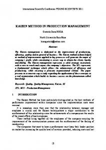
3 SAMPLE APPLICATIONS AND CONCLUSIONS In this chapter a number of sample applications will be shown to demonstrate the features and applicability of the proposed approach. In all the examples a two-dimensional shallow water flow model, and for simplicity the constant dispersion coefficient version of a depthintegrated transport model is used, in which advection is discretised via a robust upwind scheme. The first example is steady-state flow in a wide shallow channel of parabolic cross-section, with two groins and a schematised aquatic vegetation patch. Figure 1 and 2 show the velocity 3
field along with the steady-state residence time distribution displayed in grey-scale top-view and in axonometry, respectively. In fact, both of them are very unusual looking compared to other, more conventional scalar fields. In contrast to the gradual variation in the main stream, the slowly rotating recirculation zones are characterised by significantly higher residence time values. An exchange of water masses occurs then due to dispersion, first of all to its transversal component, as a result of which the water mixture in the left-hand side near-shore zone has very long volume-averaged residence time compared to the rest of the cross-section. The effect of the vegetation on the velocity field, and consequently on the residence time distribution can also be seen. The high hydraulic resistance of the vegetation results in reduced through-flow and partial diversion, making the residence time gradient locally steeper. The fact that water masses may spend some time in the recirculation zones reduces the conveyance efficiency of the studied reach, consequently at the downstream boundary the cross-sectional averaged residence time is longer than in the case without the groins. The second example is a shallow dish-shaped reservoir first with steady-state through-flow, then with superimposed wind stress pointing to the south, strong enough to induce significant changes with local gyres in the through-flow field. As can be seen in Figure 3a, the throughflow in itself produces a rather smooth residence time distribution with monotonic streamwise increase except for the low velocity near-shore zones downstream, where some slight peaks seem to develop. In the case of superimposed wind shear the changes in the flow pattern result in significant modification of the residence time field. Two large recirculation zones appear due to which the residence time of water masses increases a lot there. Water masses entrained from those zones can then increase the residence time values on their way to the outlet, as indicated in Figure 3b. The last example is a rectangular flat bottom bay with a spur dike, in which periodical flow is generated by cyclic discharge boundary condition applied at the entrance (Figure 4). Calculation over several periods was needed to reach fully time periodic system behaviour. Snapshots showing the variation of the residence time of incoming water masses over a complete cycle can be seen in Figure 5. For simplicity, the return of water masses once leaving the domain is omitted, which is in fact unlikely for such a wide entrance. In order to give some more insight into the transient space-time irregularities, the variation of the residence times is shown in Figure 6 for six representative points (indicated in Figure 4). Note the significant differences both in space and time. As to further developments, from the physical point of view advanced turbulence models can of course improve the capability to simulate the residence time evolution as much as they can the transport of water itself. The extension of the approach to other theoretical and practical cases, moreover, comparisons with Monte-Carlo-type particle tracking models are underway.
4 ACKNOWLEDGEMENTS This work was part of the project “Measurement and parameterisation of free surface flows” No. T030792 supported by the National Scientific Research Fund of Hungary.
5 REFERENCES Arnold, L., “Stochastic Differential Equations: Theory and Applications,” John Wiley and Sons, 1974.
4
Glasgow, C., A.K. Parrott, and D.C. Handscomb, “Particle Tracking Methods for Residence Time Calculations in Incompressible flow,” Oxford University Computing Laboratory, Numerical Analysis Group, Report No. 96/05, 1996. Hilton, A.B.C., D.L. McGillivary, and E.E. Adams, “Residence Time of Freshwater in Boston’s Inner Harbor,” Journal of Waterway, Port, Coastal and Ocean Engineering, ASCE, 124(2), pp. 82-89, 1998. Józsa, J., “2-D particle model for predicting depth-integrated pollutant and surface oil slick transport in rivers,” Proc. International Conference on Hydraulic and Environmental Modelling of Coastal, Estuarine and River Waters, Bradford, U.K., Gower, pp. 332-340, 1989. van Kampen, N.G., “Stochastic Processes in Physics and Chemistry,” North-Holland, Amsterdam, 1981. Koren, B., “A robust upwind discretisation method for advection, diffusion and source terms,” in Vreugdenhil, C.B., and B. Koren (eds), Numerical methods for advection diffusion problems, Vieweg, pp. 117-137, 1993. Pollock, D.W., “Semi-analytical Computation of Path Lines for Finite-Difference Models,” Ground Water, 26(6), pp. 743-750, 1988. Schafer-Perini, A.L., and J.L. Wilson, “Efficient and Accurate Front Tracking for TwoDimensional Groundwater Flow Models,” Water Resources Research, 27 (7), pp. 1471-1485, 1991. Uffink, G.J.M, “Application of the Kolmogorov’s backward equation in random walk simulations of groundwater contaminant transport,” in Kobus, W., and W. Kinzelbach (eds), Contaminant Transport in Groundwater, Balkema, 1989.
6 FIGURES
Figure 1: Residence times and velocity field in a 500 m wide channel with two groins and one vegetation patch (marked with a black frame), Q = 1000 m3/s.
5
R esidence tim e, [hours]
Figure 2: Axonometric plot of the residence times in the same channel as in Figure 1.
(a)
(b)
Figure 3: Residence times and velocity field in a dish-shaped reservoir with west-to-east through-flow only (a) and with superimposed northern wind of 15 m/s (b). P2 P1
P3
P5
Í Bay entrance P4
P6
Figure 4: Sketch of the bay with spur dike
6
Residence times, [hours]
Figure 5: Consecutive stages showing the residence times and velocity field over a complete cycle of 12 h. From top to bottom: situation at 0, 3, 6 and 9 h. 100 P1
80
P2
60
P3
40
P4 P5
20 0 0:00
P6 3:00
6:00
9:00
12:00
Cycle time
Figure 6: Residence times in six representative points during a complete discharge cycle.
7