1
Croatian Operational Research Review CRORR 5(2014), 1–13
Modelling with twice continuously differentiable functions∗ Sanjo Zlobec1,† 1
Department of Mathematics and Statistics, McGill University Burnside Hall, 805 Sherbrooke Street West, Montreal, Quebec, Canada H3A 2K6 E-mail: ⟨
[email protected]⟩ Abstract. Many real life situations can be described using twice continuously differentiable functions over convex sets with interior points. Such functions have an interesting separation property: At every interior point of the set they separate particular classes of quadratic convex functions from classes of quadratic concave functions. Using this property we introduce new characterizations of the derivative and its zero points. The results are applied to the study of sensitivity of the Cobb-Douglas production function. They are also used to describe the least squares solutions in linear and nonlinear regression. Key words: twice continuously differentiable function, zero derivative point, separation property of functions, Cobb-Douglas production function, least squares solution, Newton’s second law Invited paper, available online: March 4, 2014
1. Introduction Operations research is the study of improvable real life situations using mathematical models [11]. One of its basic topics is the identification of extreme values of functions and their corresponding optimal solutions. The classic extreme value theorem of Fermat is still widely used in various frameworks in the study of extreme points. The theorem says that a locally optimal solution can occur only at a zero-derivative point, also called a “stationary point”, e.g., [6, 11, 12]. These points have been recently characterized for continuously differentiable functions with a Lipschitz derivative and, in particular, for twice continuously differentiable functions in several variables [17, 18, 19]. The characterizations are based on the quadratic envelope property of functions introduced in [17] and they do not require infinitesimal calculus. They provide an alternative approach to the study of optimality. Let us loosely illustrate these ideas for a twice continuously differentiable function f (x) of the single variable x on an interval I = [a, b] around an interior point x∗ of I. Since f (x) is assumed to be twice continuously differentiable we know that its second derivative assumes its extreme values on I. In particular, there exists a number ρ = max |f ′′ (x)|. x∈I
∗ This
research is partly supported by NSERC of Canada. author.
† Corresponding
http://www.hdoi.hr/crorr-journal
c ⃝2014 Croatian Operational Research Society
2
Sanjo Zlobec
Following [17, 18, 19] (and Theorems 3 and 4 below) we know that an arbitrary number g = g(x∗ ) is the derivative of f at x∗ if, and only if, the ratio function |f (x) − f (x∗ ) − g · (x − x∗ )| (x − x∗ )2
(1)
is bounded on the set I \ {x∗ } = {x ∈ I, x ̸= x∗ } with an upper bound 21 ρ. For the purpose of studying sensitivity of the function we can state this result differently: An arbitrary number g = g(x∗ ) is the derivative of f at x∗ if, and only if, there exists Λ ≥ ρ (in fact, for every Λ “sufficiently large”) such that |f (x) − f (x∗ ) − g · (x − x∗ )| ≤
1 Λ(x − x∗ )2 2
(2)
for every x ∈ I. Example 1 (Verification of Derivative). Consider f (x) = x5 − x2 on I = [−1, 2] and x∗ = 0. We would like to know whether f ′ (x∗ ) = 0. Since the ratio function (1), with g = 0, is |x5 − x2 | = |x3 | x2 and it is bounded on I \ {0}, we conclude that g = f ′ (0) = 0. How about, say, x∗ = 1? Since |x5 − x2 |/(x − 1)2 → ∞ as x → 1 we conclude that at this point f ′ (x∗ ) ̸= 0. Example 2 (Sensitivity). Let us approximate f (x) = x5 − x2 on I = [−1, 2] around x∗ = 0. We know by (2) that, for a given tolerance ε > 0 1 Λ(x − x∗ )2 ≤ ε 2 implies
|f (x) − f (x∗ ) − g · (x − x∗ )| ≤ ε
for x ∈ I. One can specify Λ = ρ = 158. Therefore, since we already know that g = f ′ (0) = 0, for every x satisfying 79x2 ≤ ε we have |f (x)| ≤ ε. In particular, for the choice ε = 1, we know that |f (x)| ≤ 1| for every x such that 79x2 ≤ 1. There are real life situations which possibly cannot be improved, such as situations described by the classical laws of physics. The above results may provide different mathematical descriptions of these situations. Example 3. Consider an object of mass m moving in time along a twice continuously differentiable trajectory f (x) governed by Newton’s second law. If F (x) denotes some “force” acting on the object then on a time interval I = [a, b] the law says that F (x) = mf ′′ (x). When the force is explicitly known, one can obtain the object’s trajectory by finding a solution of this differential equation. Suppose that we do not necessarily know the force. Nevertheless, using (1) we know that for the trajectory f (x) on I and the instantaneous velocity v(x∗ ), at every moment x∗ , a < x∗ < b the ratio function |f (x) − f (x∗ ) − v(x∗ ) · (x − x∗ )| (x − x∗ )2
Modelling with twice continuously differentiable functions
3
is bounded on the set I \ {x∗ }. After specifying Λ = ρ in (2), a bound is 1 1 1 1 Λ = ρ = max |f ′′ (x)| = max |F (x)|. 2 2 2 x∈I 2m x∈I In particular, if the object is moving with a constant velocity, then ρ = 0 and we conclude that its position is f (x) = f (x∗ ) + v(x∗ ) · (x − x∗ ) at every x ∈ I. It is easy to verify these properties for the trajectory of an object during its free fall. The preceding examples show that the new characterizations of the derivative may not always be suitable for calculating the derivative but they have three applications. They can be used to verify (rather than calculate) the derivative, determine a region around a given x∗ where all values of the function fall within a specified tolerance, and one can possibly use them to learn more about the model. The objective of this paper is to extend some of the recent results for functions of the single variable to functions in several variables. The extensions will be illustrated on the Cobb-Douglas production function in economics and also in regression. In particular, we obtain new characterizations of partial derivatives of the production function, which are important to study sensitivity of the model, and new characterizations of the best least squares solutions. These illustrations have different mathematical properties. The Cobb-Douglas function is studied around non-zero derivative points and therefore the related problems are well posed [13, 14]. In contrast, the least squares problems generally are ill posed and they are also known to be notoriously ill conditioned [2]. We will not study numerical topics. In optimization these are studied in, e.g., [4] and [7]. Mathematical background of the paper is set at the level of intermediate calculus and linear algebra. The most recent material related to this paper can be found in [19].
2. Separation of functions Consider a twice continuously differentiable (abbreviated: C 2 ) function f in n variables on a closed and bounded (abbreviated: compact) convex set K with interior points. Denote by H = ∇2 f (x) the Hessian matrix of f at x and by λi = λi (x) its i-th eigenvalue, i = 1, . . . , n. Since the eigenvalues of H are real numbers we can introduce the “global” spectral radius of H on K, denoted by ρ = max max |λi |. x∈K i=1,...,n
This is a non-negative number which depends on H and K. It makes the function f (x) + 21 ρ||x2 || convex. Here ||x|| denotes the Euclidean norm of a column n-tuple x. In fact, one has a more general claim. Theorem 1. Consider a C 2 function f in n variables on a compact convex set K in its open domain and the global spectral radius ρ of its Hessian matrix on K. Then for every number Λ ≥ ρ, the function f (x) + 12 Λ||x2 || is convex on K and the function f (x) − 21 Λ||x2 || is concave on K.
4
Sanjo Zlobec
Proof. The function f (x) + 12 Λ||x2 || is convex on K if, and only if, the matrix ∇2 f (x) + ΛI, where I is the n × n unit matrix, is positive semi-definite for every x ∈ K. Using the transpose uT of u, and matrix multiplication, this is equivalent to uT ∇2 f (x)u + Λ ≥ 0, ||u2 || for every u ̸= 0. Since Λ ≥ ρ, we have λi (x) + ρ ≥ 0, and it follows that λi (x) + Λ ≥ 0, i = 1, . . . , n. Hence we conclude that f (x) + 12 Λ||x2 || is convex. Similarly one can prove the concavity part. Example 4. If f is a C 2 function of the single variable on an interval I = [a, b], then ρ = max |f ′′ (x)|. x∈I
This number was introduced in Section 1. For f (x) = sin x on I = [−π, π], it is ρ = 1. For the product function f (x) = x1 x2 , the eigenvalues of the Hessian matrix on any compact convex set K are λ1 = −1 and λ2 = 1, hence ρ = 1. We use ρ to describe a separation property of C 2 functions. Theorem 2 (Separation property of C 2 functions). Consider a C 2 function f (x) in n variables defined on an open set of Rn containing a compact convex set K. Denote by ρ the global spectral radius of the Hessian matrix of f on K. Take an arbitrary interior point x∗ of K and denote by G = ∇f (x∗ ) the gradient of f at x∗ . Then for every number Λ such that Λ ≥ ρ, we have 1 1 − Λ||x − x∗ ||2 +f (x∗ )+G·(x − x∗ ) ≤ f (x) ≤ f (x∗ )+G·(x − x∗ )+ Λ||x − x∗ ||2 (3) 2 2 for every x ∈ K. Proof. We know, forΛ ≥ ρ, that C(x, Λ) = f (x) + 21 Λ||x||2 is a convex function on K, by Theorem 1. Therefore, for x and x∗ in K, we have C(λx + (1 − λ)x∗ , Λ) ≤ λC(x, Λ) + (1 − λ)C(x∗ , Λ) for every 0 ≤ λ ≤ 1. Hence f (λx + (1 − λ)x∗ ) ≤
1 1 Λ||λx + (1 − λ)x∗ ||2 + λf (x) − Λλ||x||2 2 2 1 +(1 − λ)f (x∗ ) + Λ(1 − λ)||x∗ ||2 . 2
Using properties of the norm, and after division by λ > 0, this yields 1 f (x∗ + λ(x − x∗ )) − f (x∗ ) ≤ f (x) − f (x∗ ) + Λ(1 − λ)||x − x∗ ||2 . λ 2 On the left-hand side we have a quotient of functions in the single variable λ of the type 00 . Using L’Hopital’s rule, in the limit λ → 0 this becomes 1 ∇f (x∗ ) · (x − x∗ ) ≤ f (x) − f (x∗ ) + Λ||x − x∗ ||2 . 2
5
Modelling with twice continuously differentiable functions
˜ Λ) = f (x) − 1 Λ||x||2 is a concave function, it follows that Similarly, since C(x, 2 1 ∇f (x∗ ) · (x − x∗ ) ≥ f (x) − f (x∗ ) − Λ||x − x∗ ||2 . 2
Theorem 2 gives relationships between a C 2 function and its first and second derivatives. The second derivative enters the inequalities indirectly through ρ. Example 5. Consider f (x) = sin x on a compact interval and its interior point x∗ . The separation property, after specifying Λ = ρ and ρ = 1, says that 1 1 − (x − x∗ )2 + sin x∗ + cos x∗ · (x − x∗ ) ≤ sin x ≤ sin x∗ + cos x∗ · (x − x∗ ) + (x − x∗ )2 2 2 for every x ∈ I. At x∗ = 0 this yields 1 1 x − x2 ≤ sin x ≤ x + x2 2 2
for
− π ≤ x ≤ π.
The choice of a smaller interval, e.g., I = [− π4 , π4 ] and ρ = 12 maxx∈I |f ′′ (x)| = yields √ √ 2 2 2 2 π π x− x ≤ sin x ≤ x + x for − ≤ x ≤ . 4 4 4 4
√
2 4
The separation is depicted in Figure 1 on the region − π2 ≤ x, x∗ ≤ π2 by an “extended graph” of f (x) in the space with coordinates (x, x∗ ); function sin x is represented in that space as sin x + 0 · x∗ .
Figure 1: Separating property of sine function
6
Sanjo Zlobec
The inequalities (3) can be written in a more concise form using the absolute value function. For f (x) on K we introduce its “extension function” around an interior point x∗ of K as E(x, x∗ ) =
|f (x) − f (x∗ ) − ∇f (x∗ ) · (x − x∗ )| , ||x − x∗ ||2
x ∈ K \ {x∗ } = {x ∈ K, x ̸= x∗ }.
Theorem 2 says that E(x, x∗ ) is bounded on the set K \ {x∗ } by 12 ρ. Example 6. Consider f (x) = x1 x2 on K = {(x1 , x2 )T : −1 ≤ x1 , x2 ≤ 1}. Its extension function around x∗ = 0 is E(x, x∗ ) =
|x1 x2 | . x21 + x22
Since ρ = 1, by Example 4, an upper bound of E(x, x∗ ) on K \ {x∗ } is 12 . The graph of this function is depicted in a different context in [19]. Theorem 2 can also be used to find lower bounds of the global spectral radius. Example 7. Consider the product function f (x) = x1 x2 · · · xn in n ≥ 2 variables on a compact convex set K in Rn containing x∗ = 0 in its interior. Since G = ∇f (x∗ ) = 0, (3) gives a lower bound of the global spectral radius ρ of the Hessian matrix of f on K 2x1 x2 · · · xn ≤ ρ for every x = (xi ) ̸= 0. 2 x1 + x22 + · · · + x2n In particular, for n = 2, the inequality is obvious. But it is not obvious for n ≥ 3.
3. Characterizations of the gradient and its zero points The well-known geometric property of the gradient of f (x) at x∗ is that it is an ntuple in Rn orthogonal to the level set {x : f (x) = f (x∗ )} at x∗ and pointing in the direction of steepest ascent of f from x∗ . This property is used in the classic steepest ascent method of Cauchy and in its many variations and numerical improvements. In mathematical modelling it is used to describe many interesting situations such as flight of insects toward a light source, trajectory of a heat-seeking missile and movements of sharks in water towards higher blood concentration [1]. In this section we will use Theorem 2 to give an essentially different property of the gradient. In fact, we will characterize the gradient. Theorem 3 (Global characterization of the gradient). Consider a C 2 function f (x) in n variables defined on an open set of Rn containing a compact convex set K with a nonempty interior. Also consider the global spectral radius ρ of the Hessian matrix of f on K and a number Λ, Λ ≥ ρ. A row n-tuple G = G(x∗ ) is the gradient of f at an interior point x∗ of K if, and only if, the inequalities (3) hold for every x ∈ K. Proof. In view of Theorem 2, we only have to show that G in (3), is represented by an n-tuple of partial derivatives. This can be seen after dividing (3) by ||x − x∗ || = ̸ 0 where x ̸= x∗ is chosen on the i-th coordinate axis. The i-th component of G = (Gi ),
Modelling with twice continuously differentiable functions
in the limit x → x∗ , is the partial derivative gradient of f at x∗ .
∂f ∗ ∂xi (x ), i
7
= 1, . . . , n. Hence G is the
Theorem 3 can be formulated differently using the extension function of f . Theorem 4 (Uniform bound characterization of the gradient). Consider a C 2 function f (x) in n variables defined on an open set of Rn containing a compact convex set K with a nonempty interior. Also consider the global spectral radius ρ of the Hessian matrix of f on K and a number Λ, Λ ≥ ρ. A row n-tuple G = G(x∗ ) is the gradient of f at an interior point x∗ of K if, and only if |f (x) − f (x∗ ) − G · (x − x∗ )| 1 ≤ Λ ∗ 2 ||x − x || 2
(4)
for every x ∈ K \ {x∗ }. Let us illustrate Theorem 4. Example 8. Consider f (x) = x0.4 on the interval I = [2, 4]. Take x∗ = 3. Is f ′ (3) = 0.2? Since the left-hand side in (4), with G = 0.2, is not bounded on the set I \ {3} because |x0.4 − 30.4 − 0.2(x − 3)| → ∞ as x → 3 (x − 3)2 we conclude that f ′ (3) ̸= 0.2. This situation is depicted in Figure 2.
Figure 2: Incorrect derivative
Is f ′ (3) = 0.4? Since the ratio function |x0.4 − 30.4 − 0.4(x − 3)| (x − 3)2
8
Sanjo Zlobec
Figure 3: Correct derivative
is bounded on I \ {3} we conclude that f ′ (3) = 0.4. This situation is depicted in Figure 3. Warning. Theorems 3 and 4 do not generally hold for continuously differentiable functions. A counter example is f (x) = |x|3/2 on I = [−1, 1] considered around x∗ = 0, [17]. Theorem 3 can also be used to estimate values of functions around a given point x∗ falling within a prescribed tolerance ε ≥ 0. Let us follow-up on Example 2 for functions in several variables. Theorem 5. Consider a C 2 function f (x) in n variables defined on an open set of Rn containing a compact convex set K with nonempty interior. Let ρ > 0 be the global spectral radius of the Hessian matrix of f on K and take Λ ≥ ρ. Consider an interior point x∗ of K. Then for a given ε ≥ 0 |f (x) − f (x∗ ) − ∇f (x∗ ) · (x − x∗ )| ≤ ε
whenever
||x − x∗ ||2 ≤
2ε , x ∈ K. Λ
Example 9. Consider f (x) = cos x around x∗ = 0. Here ρ = 1 and we can take Λ = 1. Therefore for any tolerance ε ≥ 0, we know that |1 − cos x| ≤ ε, for every x which satisfies x2 ≤ 2ε. In general, the bigger choice of Λ, the smaller interval for estimation. Theorems 3 and 4 yield, in particular, characterizations of zero-derivative points ∇f (x∗ ) = 0. One only specifies G = 0 in the theorems. One can find illustrations of this special case in, e.g., [12, 17, 18, 19].
Modelling with twice continuously differentiable functions
9
4. Cobb-Douglas production models The Cobb-Douglas models are formulated as products of several functions each of the single variable xi raised to some constant powers ai , i = 1, . . . , k. In economics, they might represent the technological relationships between k different inputs such as capital and labour and the amount of output that is produced by these inputs. The results from the preceding sections are directly applicable to these models to verify derivatives and study sensitivity under input perturbations. Let us outline how this can be done on an example borrowed from [12, p. 291] with the original notation. Example 10. Consider the Cobb-Douglas production model Q(L, K) = 100L0.4 K 0.6 studied around L∗ = 1024 and K ∗ = 32768. Here Q denotes total production (the real value of all goods produced in, say, a year, L denotes labour input (the total number of person hours worked in a year), K denotes capital input (the real value of all machinery, equipment, and buildings), 0.4 and 0.6 are the output elasticities of capital and labour respectively. Constant A = 100 is total factor productivity. ∗ ∗ ∗ ,K ∗ ) The partial derivatives are found to be ∂Q(L∂L,K ) ≈ 320 and ∂Q(L ≈ 15. This ∂K means that, at K ∗ , if L∗ is increased from 1024 to 1025, Q is roughly estimated to increase by 320. Similarly, at the fixed L∗ , if K is increased from 32768 to 32769, Q is estimated to increase by 15. The extended function of Q(L, K) around L∗ and Q∗ is the ratio function E(L, K, L∗ , K ∗ ) =
|Q(L, K) − Q(L∗ , K ∗ ) − (320, 15)(L − L∗ , K − K ∗ )T | (L − L∗ )2 + (K − K ∗ )2
where (L, K) ̸= (L∗ , K ∗ ) in a compact convex set containing (L∗ , K ∗ ) in its interior. Its graph is depicted by Figure 4.
Figure 4: Extended Cobb-Douglas function around fixed inputs
10
Sanjo Zlobec
For the results to be meaningful, the function E(L, K, L∗ , K ∗ ) should be bounded on every compact convex set around (L∗ , K ∗ ). From the graph (done in MATLAB) we see that the bound has the value about 200. This implies that the global spectral radius ρ of the Hessian matrix on the chosen region in (L, K) around (L∗ , K ∗ ) is about 400. One can use this information for a more refined sensitivity analysis using Theorem 5. Finer the grid in the (L, K) plane, smoother is the shape of the graph and more accurate are the estimates of ρ and perturbed values of the function. Partial derivatives of a general Cobb-Douglas function f (x1 , . . . , xk ), at a given ∂f (x∗ ) input x∗i are Gi = ∂xii , i = 1, . . . , k. They can be verified directly using Theorems 3 and 4 if we study the k “coordinate-wise” functions of the single variable: f (x1 , x∗2 , . . . , x∗k ), . . . , f (x∗1 , . . . , x∗k−1 , xk ). Since the model is stated in terms of C 2 functions and studied around non-zero inputs, the verifications of the derivatives and study of sensitivity are well posed problems according to the general results given in [13] and [14].
5. Regression Theorems 3 and 4 can be used in linear regression to characterize least squares solutions of possibly inconsistent systems of linear algebraic equations Ax = b. For a given m × n matrix A and an m-tuple b, consider the function F (x) = ||Ax − b||2 . The Hessian matrix of F (x) is ∇2 F (x) = 2AT A which is positive semi definite. Therefore F (x) is a convex function regardless of the choice of A and b. Its optimal solution x∗ is called a least squares solution. It is a zero-derivative point of F (x) so let us use, e.g., Theorem 4 for its characterization. Denote by σ the largest eigenvalue of AT A. Theorem 6 (Characterization of least squares solutions). An n-tuple x∗ is a least squares solution of Ax = b if, and only if | ||Ax − b||2 − ||Ax∗ − b||2 | ≤σ ||x − x∗ ||2
(5)
on the set K \ {x∗ }, where K is an arbitrary compact convex set containing x∗ in its interior. Example 11 (Trivial example). Consider Ax = b where A = 0 is the m × n zero matrix. Any n-tuple x∗ is its least squares solution. Remark 1. Theorem 6 can be formulated using properties of generalized inverses of matrices, e.g., [2, 8, 15]. In particular, the term Ax∗ − b is the orthogonal projection of b on the null space of AT . Example 12 (Estimating number of divorces in Canada in 1890). The number of registered divorces in Canada from 1880 to 1889 is given by the following data according to the “Statistical Year-book of Canada 1902”: Year (ti ) 1880 1881 1882 1883 1884 1885 1886 1887 1888 1889 . Divorces (di ) 5 7 6 13 10 12 11 10 9 15
Modelling with twice continuously differentiable functions
11
Using linear regression we wish to estimate the number of divorces in 1890. The ten years can be ordered from, say, 1 to 10 instead of 1880 to 1889. The linear regression line can be assumed to be of the form d = x1 t + x2 . Passing this line through the ten points gives a system Ax = b of 10 equations in 2 unknowns where [ ] 1 2 3 4 5 6 7 8 9 10 T , A = 111111111 1 [ ] bT = 5 7 6 13 10 12 11 10 9 15 . The least squares solution x∗ = (x∗1 , x∗2 ) is calculated to be x∗1 = 0.73, x∗2 = 5.8. Hence the regression line is d = 0.73t + 5.8 and the estimated number of divorces in 1890 is d = 0.73 · 11 + 5.8 = 13.83 ≈ 14. The result can be verified using Theorem 6. An upper bound of the ratio function in (5) on any compact convex set containing x∗ in its interior is σ = 392.90. In general, the “error function” F (x) can be any C 2 function. If data (di , ti ), i = 1, . . . , N in the (d, t) plane are approximated by, say, the exponential function d = x 1 · ex 2 t describing, e.g., radioactive decay, then passing this function through the N points yields a generally inconsistent system of N equations in two variables. The error function could be of the form ∑ F (x) = (di − x1 · ex2 ti )2 . i=1,...,N
The nonlinear least squares problem here is to find minimizing points x∗ = (x∗1 , x∗2 ) of F (x). At these points the derivative of F (x) must be equal to zero. One can use Theorems 3 and 4 with G = 0 to characterize zero-derivative points. Interesting approximations of data by exponential functions were described in [9] and [10]. The measurements were done in vivo on patients using positron emission tomography after radioactive tissue tracer was administered into the patients’ “vascular space”. Also the influence of scan intervals on improvement of “parameter estimates” (x∗ in minimization of the error function) was studied. In the context of input optimization [16] the problem of finding “best scanning intervals” can be identified as a problem of finding “optimal inputs”. Indeed, in input optimization some or all data are identified as a vector input θ. The error function is thus formulated in terms of x and θ, i.e., as some F = F (x, θ). The problem is to find a particular θ∗ which minimizes the optimal value function F ◦ (θ) = F (x∗ (θ), θ) subject to constraints imposed on x and θ. Here x∗ (θ) is an optimal solution of F (x, θ) for a given θ. This x∗ (θ) can be calculated by a method of “robust optimization” [3], which may take into consideration stochastic nature of data. Characterizations of “optimal inputs” θ∗ over “regions of stability” for convex parametric models are formulated in [16] using suitable Lagrange functions. The study of optimal inputs is important in many applied areas including designs of experiments [5].
12
Sanjo Zlobec
6. Conclusion We have studied some of the basic problems in mathematical modeling using twice continuously differentiable functions. One of these problems is how to characterize the derivative and its zero points. We have found these characterizations using a separating property of functions. The new results are based on the global quadratic envelope property of functions and they do not explicitly require infinitesimal calculus. One can use them to verify solutions of mathematical models which use derivatives. They can also be used to study the model’s sensitivity to data and, in some cases, to reformulate the model. The results are applied to the Cobb-Douglas production model and to linear and nonlinear regression. In these applications we have obtained equivalent, but geometrically different, characterizations of partial derivatives of the Cobb-Douglas function and we have characterized least squares solutions in linear regression.
Acknowledgement The author is indebted to his colleagues for their constructive comments. In particular, Adi Ben-Israel made valuable remarks on Theorem 6 which clarified and improved its presentation. The author is indebted to Mirko Dikˇsi´c for many discussions of the research topics related to regression which were implemented at Brain Imaging Center at McGill University. He has also provided the author with related references. Biagio Ricceri has communicated to the author his latest research on well-posed problems. Also many thanks go to Ivan Soldo for his patience and technical support.
References [1] Barkey, D. D. (1984). Calculus. Saunders College Publishing. Philadelphia. [2] Ben-Israel, A and Greville T. N. (2013). Generalized Inverses: Theory and Applications. CMS Books in Mathematics. Second edition. Springer. [3] Ben-Tal, A. and Nemirovski A. (1998). Robust convex optimization. Math. Oper. Res., 23, 769–805. [4] Bertsekas, D. P. (1979). Convexification procedures and decomposition methods for nonconvex optimization problems. J. Optim. Theory Appl., 29, 169–197. [5] Box, G. E. P. and Lucas H. L. (1959). Design of experiments in nonlinear situations. Biometrica, 46, 77–99. [6] Crnjac, M., Juki´c, D. and Scitovski, R. (1994). Matematika. Faculty of Economics. University of Osijek. [7] Floudas, C. A. and Gounaris, C. E. (2009). An overview of advances in global optimization during 2003-2008. A chapter in the book Lectures on Global Optimization. Pardalos, P. M. and Coleman, T. F. (Eds.). Fields Institute Communications. Vol. 55, 105–154. [8] Golan, J. S. (2011). The Linear Algebra a Beginning Graduate Student Ought to Know. Third edition. Springer. [9] Jovkar, S., Evans, A. C., Dikˇsi´c, M., Nakai, H., and Yamamoto, Y. L. (1989). Minimisation of parameter estimation errors in dynamic PET: choice of scanning schedules. Phys. Med. Biol., 34, 895–908.
Modelling with twice continuously differentiable functions
13
[10] Kato, A., Dikˇsi´c, M., Yamamoto, Y. L., Strother, S. C. and Feindel, W. (1984). An improved approach for measurement of regional celebral rate constants in the deoxy glucose method with positron emission tomography. J. Celebral Blood Flow and Metabolism, 4, 555–563. [11] Lukaˇc, Z. and Nerali´c, L. (2012). Operacijska Istraˇzivanja. Zagreb: Element. ˇ [12] Nerali´c, L. and Sego, B. (2013). Matematika. Second edition. Zagreb: Element. [13] Ricceri, B. (2007). The problem of minimizing locally a C 2 functional around noncritical points is well posed. Proceedings of the American Mathematical Society, 135, 2187–2191. [14] Ricceri, B. (2012). A strict minimax inequality criterion and some of its consequences. Positivity, 16, 455–470. [15] Zlobec, S. (1970). An explicit form of the Moore-Penrose inverse of an arbitrary complex matrix. SIAM Review, 12, 132–134. [16] Zlobec, S. (2001). Stable Parametric Programming. Boston: Kluwer. [17] Zlobec, S. (2010). Characterizing zero-derivative points. J. Global Optim., 46, 155– 161. [18] Zlobec, S. (2011). Alternative formulations of the gradient. J. Global Optim., 46, 549–553. [19] Zlobec, S. (2014). Separating property of continuously differentiable functions. To appear in Math. Commun.