Models and Algorithms for Railway Line Planning

2

MODELS AND ALGORITHMS FOR RAILWAY LINE PLANNING PROBLEMS Jan-Willem Goossens

Models and Algorithms for Railway Line Planning Problems

Jan-Willem Goossens

Models and Algorithms for Railway Line Planning Problems Proefschrift

ter verkrijging van de graad van doctor aan de Universiteit Maastricht, op gezag van de Rector Magnificus, Prof. mr. G.P.M.F. Mols volgens het besluit van het College van Decanen, in het openbaar te verdedigen op woensdag 24 november 2004 om 16.00 uur

door

Jan-Willem Henricus Mathijs Goossens

Promotoren: Prof. dr. ir. C.P.M. van Hoesel Prof. dr. L.G. Kroon (Erasmus Universiteit Rotterdam)

Beoordelingscommissie: Prof. dr. ir. A.W.J. Kolen (voorzitter) Dr. J.J. van de Klundert Prof. dr. A.P.M. Wagelmans (Erasmus Universiteit Rotterdam) Prof. dr. D. Wagner (Universit¨ at Karlsruhe)

Models and Algorithms for Railway Line Planning Problems c

2004, Jan-Willem H.M. Goossens Proefschrift Universiteit Maastricht ISBN 90-9018605-0 Het in dit proefschrift beschreven onderzoek werd mede mogelijk gemaakt door NS Reizigers B.V. en het onderzoeksnetwerk AMORE van de Europese Unie.

Acknowledgements On the first of November 1998, now almost six years ago, I started my research as a PhD candidate at the University of Maastricht. Within these very interesting six years I presented at a range of international conferences, taught courses for students, obtained my LNMB diploma, moved to Konstanz in Germany—and back again—and, of course, spent a lot of time doing research, and writing this thesis. My position was made possible by a research agreement between the Dutch passenger railway operator NS Reizigers and the University of Maastricht. This agreement was the brainchild of my supervisors Stan van Hoesel and Leo Kroon. In the first place, I would like to express my gratitude to them for making all of this possible. Through Leo’s involvement in the EU project for Algorithmic Methods for Optimizing the Railways in Europe, I came into contact with a number of other participating groups, and visited several of their workshops. On one of these meetings, after a nice evening with pizzas, good wines and a discussion with Dorothea Wagner of the Universit¨at Konstanz, Leon Peeters and I reached the conclusion that a long visit to the group in Konstanz would be a good opportunity to do research, work on our theses, learn to speak German, and, on the side, go snowboarding on winter weekends. On April 1st 2002 this plan came into realisation when, with an eleven months leave from the University of Maastricht, I moved to the beautifully small city of Konstanz. I would like to thank Dorothea for giving me this opportunity. In addition, I wish to thank all the members of the Algorithms and Datastructures Group for their warm welcome and the interesting time I spent there. Furthermore, I am grateful to all of those who took the time to proofread different parts of my thesis over and over again. For this I would particularly like to thank Leo Kroon, Stan van Hoesel, Leon Peeters and Anton van der Kraaij. I am also grateful to all the members of the Department of Quantitative Economics. With the numerous questions that I’ve had over the last six years, the mix of colleagues within the department proved to be very valuable. Finally, I would like to express a lot of thanks to my family and friends, in particular to my parents and to Nathalie for their unconditional and generous support. Maastricht, September 2004 Jan-Willem Goossens

i

Contents Acknowledgements

i

Contents

iii

List of Tables

vii

List of Figures

ix

1 Introduction 1.1 Past to present situation in the Netherlands 1.2 Future developments . . . . . . . . . . . . . 1.2.1 Increasing reliability . . . . . . . . . 1.2.2 Increasing capacity . . . . . . . . . . 1.3 Planning problems for passenger railways . 1.3.1 Estimating passenger demand . . . . 1.3.2 Line planning . . . . . . . . . . . . . 1.3.3 Timetabling . . . . . . . . . . . . . . 1.3.4 Platform and track assignment . . . 1.3.5 Rolling stock planning . . . . . . . . 1.3.6 Crew scheduling . . . . . . . . . . . 1.3.7 Shunting and maintenance planning 1.4 The overall planning process at NSR . . . . 1.4.1 Current planning stages . . . . . . . 1.4.2 Proposed planning process . . . . . . 1.5 An introduction to line planning . . . . . . 1.6 Research objective . . . . . . . . . . . . . . 1.7 Outline of this thesis . . . . . . . . . . . . .

I

Foundations

. . . . . . . . . . . . . . . . . .

. . . . . . . . . . . . . . . . . .

. . . . . . . . . . . . . . . . . .

. . . . . . . . . . . . . . . . . .

. . . . . . . . . . . . . . . . . .

. . . . . . . . . . . . . . . . . .

. . . . . . . . . . . . . . . . . .

. . . . . . . . . . . . . . . . . .

. . . . . . . . . . . . . . . . . .

. . . . . . . . . . . . . . . . . .

. . . . . . . . . . . . . . . . . .

. . . . . . . . . . . . . . . . . .

. . . . . . . . . . . . . . . . . .

. . . . . . . . . . . . . . . . . .

. . . . . . . . . . . . . . . . . .

1 1 2 3 3 4 5 5 5 6 7 9 10 11 11 12 14 15 17

19

2 Combinatorial foundations 21 2.1 Polyhedral combinatorial optimisation . . . . . . . . . . . . . . . . . . 21 2.1.1 Combinatorial optimisation problems . . . . . . . . . . . . . . . 21 iii

iv

CONTENTS . . . . .

. . . . .

. . . . .

. . . . .

. . . . .

. . . . .

. . . . .

. . . . .

. . . . .

. . . . .

. . . . .

. . . . .

. . . . .

22 23 24 29 31

3 Foundations in line planning modelling 3.1 Line plans and cyclic timetables . . . . . . . . . . 3.2 Rolling stock . . . . . . . . . . . . . . . . . . . . 3.3 Passenger demand . . . . . . . . . . . . . . . . . 3.3.1 Passenger demand and capacity planning 3.3.2 Passenger demand across the network . . 3.3.3 Passenger demand variations over time . . 3.4 Infrastructure . . . . . . . . . . . . . . . . . . . . 3.4.1 Station capacity . . . . . . . . . . . . . . 3.4.2 Homogenising the train system . . . . . . 3.4.3 New railway safety systems . . . . . . . . 3.5 Modelling the railway system . . . . . . . . . . . 3.5.1 Infrastructure . . . . . . . . . . . . . . . . 3.5.2 Lines . . . . . . . . . . . . . . . . . . . . . 3.5.3 Rolling stock . . . . . . . . . . . . . . . .

. . . . . . . . . . . . . .

. . . . . . . . . . . . . .

. . . . . . . . . . . . . .

. . . . . . . . . . . . . .

. . . . . . . . . . . . . .

. . . . . . . . . . . . . .

. . . . . . . . . . . . . .

. . . . . . . . . . . . . .

. . . . . . . . . . . . . .

. . . . . . . . . . . . . .

. . . . . . . . . . . . . .

. . . . . . . . . . . . . .

33 33 34 35 35 39 39 40 40 41 42 44 44 44 46

2.2 2.3

II

2.1.2 Polyhedral theory . . . . . . . . . . . 2.1.3 Integer linear programming problems . 2.1.4 Solution approaches . . . . . . . . . . Multi-commodity flows . . . . . . . . . . . . . Theoretical overview . . . . . . . . . . . . . .

. . . . .

Applications

4 Branch-and-cut for line planning problems 4.1 Introduction . . . . . . . . . . . . . . . . . . 4.2 Model formulation . . . . . . . . . . . . . . 4.2.1 Formulation . . . . . . . . . . . . . . 4.3 Branch-and-cut method for CLP . . . . . . 4.3.1 Preprocessing . . . . . . . . . . . . . 4.3.2 Cutting planes . . . . . . . . . . . . 4.3.3 Tree search . . . . . . . . . . . . . . 4.4 Implementation issues . . . . . . . . . . . . 4.4.1 Preprocessing implementation . . . . 4.4.2 Cutting planes implementation . . . 4.4.3 Branching rules implementation . . . 4.5 Computational results . . . . . . . . . . . . 4.5.1 Unbounded computation times . . . 4.6 Summary and conclusions . . . . . . . . . .

49 . . . . . . . . . . . . . .

. . . . . . . . . . . . . .

. . . . . . . . . . . . . .

. . . . . . . . . . . . . .

. . . . . . . . . . . . . .

. . . . . . . . . . . . . .

. . . . . . . . . . . . . .

. . . . . . . . . . . . . .

. . . . . . . . . . . . . .

. . . . . . . . . . . . . .

. . . . . . . . . . . . . .

. . . . . . . . . . . . . .

51 51 52 53 54 55 60 65 67 67 68 70 71 76 76

5 The multiple-type line planning problem 5.1 Modelling . . . . . . . . . . . . . . . . . . . . . . . 5.1.1 Definitions and notation . . . . . . . . . . . 5.2 Formulating the multi-type line planning problem . 5.3 Formulations for the edge capacity problem . . . .

. . . .

. . . .

. . . .

. . . .

. . . .

. . . .

. . . .

. . . .

. . . .

. . . .

. . . .

79 79 80 82 83

. . . . . . . . . . . . . .

. . . . . . . . . . . . . .

. . . . . . . . . . . . . .

CONTENTS

5.4 5.5

v

5.3.1 The multi-commodity flow formulation . . . . 5.3.2 The mixed integer programming formulation 5.3.3 The integer programming formulation . . . . Computational results . . . . . . . . . . . . . . . . . Summary and conclusions . . . . . . . . . . . . . . .

6 The station type optimisation problem 6.1 Introduction . . . . . . . . . . . . . . . . . . 6.2 Modelling . . . . . . . . . . . . . . . . . . . 6.2.1 The line-event graph . . . . . . . . . 6.2.2 Valid paths in the line-event graph . 6.3 Problem formulation . . . . . . . . . . . . . 6.3.1 Extending the STOP(t¯) formulation 6.4 Lagrangian relaxation . . . . . . . . . . . . 6.5 The branch-and-bound algorithm . . . . . . 6.5.1 Preprocessing . . . . . . . . . . . . . 6.5.2 Bounding methods . . . . . . . . . . 6.5.3 Tree search . . . . . . . . . . . . . . 6.6 Computational results . . . . . . . . . . . . 6.6.1 Comparing line plans . . . . . . . . 6.7 Summary and conclusions . . . . . . . . . .

. . . . . . . . . . . . . .

. . . . . . . . . . . . . .

. . . . . . . . . . . . . .

. . . . . . . . . . . . . .

. . . . . . . . . . . . . .

. . . . .

. . . . .

. . . . .

. . . . .

. . . . .

. . . . .

. . . . .

. . . . .

. . . . .

. . . . .

83 88 92 97 100

. . . . . . . . . . . . . .

. . . . . . . . . . . . . .

. . . . . . . . . . . . . .

. . . . . . . . . . . . . .

. . . . . . . . . . . . . .

. . . . . . . . . . . . . .

. . . . . . . . . . . . . .

. . . . . . . . . . . . . .

. . . . . . . . . . . . . .

. . . . . . . . . . . . . .

103 103 104 104 108 109 111 112 114 114 119 122 123 130 130

A Appendix for Chapter 1

133

B Appendix for Chapter 4

135

C Appendix for Chapter 5

137

D Appendix for Chapter 6

139

Bibliography

149

Index

157

Samenvatting (Summary in Dutch)

161

Curriculum Vitæ

165

List of Tables 4.1 4.2 4.3 4.4 4.5 4.6

Characteristics of the instances. . . . . . . . . . . . . . . . . Preprocessing results for variable and constraint reduction. Statistics for the individual classes of cutting planes. . . . . Statistics for the branching rules. . . . . . . . . . . . . . . . Computational results. . . . . . . . . . . . . . . . . . . . . . Cut-and-branch without time restrictions. . . . . . . . . . .

. . . . . .

. . . . . .

. . . . . .

. . . . . .

. . . . . .

. . . . . .

71 72 72 72 75 76

5.1 5.2 5.3 5.4 5.5

Variable and constraint statistics per formulation. . . Characteristics of the instances. . . . . . . . . . . . . . Statistics for the different instances and formulations. Computational results. . . . . . . . . . . . . . . . . . . Comparing CLP and MCLP solutions. . . . . . . . . .

. . . . .

. . . . .

. . . . .

. . . . .

. . . . .

. . . . .

97 98 98 100 100

6.1 6.2 6.3 6.4 6.5 6.6 6.7 6.8

Characteristics of the instances. . . . . . . . . . . . . . . . . . . . Initial statistics before preprocessing. . . . . . . . . . . . . . . . . Statistics after preprocessing. . . . . . . . . . . . . . . . . . . . . Statistics for the root node of the branch-and-bound tree. . . . . Branch-and-bound statistics for the branching rules. . . . . . . . Results of applying the MAA and RVA techniques at every node. Comparing the current and new total travel times. . . . . . . . . Statistics for the MCLP line plans. . . . . . . . . . . . . . . . . .

. . . . . . . .

. . . . . . . .

. . . . . . . .

123 125 125 126 128 129 129 130

. . . . .

. . . . .

. . . . .

D.1 Statistics for the original STOP formulation. . . . . . . . . . . . . . . 142 D.2 Solution statistics. . . . . . . . . . . . . . . . . . . . . . . . . . . . . . 145

vii

List of Figures 1.1 1.2 1.3 1.4 1.5 1.6 1.7 1.8 1.9 1.10

Planning problems. . . . . . . . . . . . . . . . . . . . . . . . . . . . . Time-space diagram for the tracks between Rotterdam and Utrecht. An example of a platform assignment for the station Utrecht. . . . . An example of a rolling stock assignment. . . . . . . . . . . . . . . . A Gannt chart with duties. . . . . . . . . . . . . . . . . . . . . . . . An example of a station layout of the station Zwolle. . . . . . . . . . The current planning process. . . . . . . . . . . . . . . . . . . . . . . The new planning process concept. . . . . . . . . . . . . . . . . . . . Line plan of the underground system in London. . . . . . . . . . . . How to get from Gloucester Road to Westbourne Park. . . . . . . .

2.1 2.2

Two types of hulls for the two points x1 = (1, 2) and x2 = (3, 1) from R2 . 22 The feasible points, their convex hull, and the LP polytope. . . . . . . 25

3.1 3.2 3.3 3.4 3.5 3.6 3.7 3.8

Different types of rolling stock. . . . . . . . . . . . . . . . . An example origin-destination matrix. . . . . . . . . . . . . The percentage of all travellers grouped by travel distance. The number of travellers at different points in time. . . . . The current situation and four proposed modifications. . . . The current situation and the moving block safety system. . The Dutch and German railway networks. . . . . . . . . . . Trains versus frequency. . . . . . . . . . . . . . . . . . . . .

4.1 4.2 4.3 4.4 4.5 4.6

The Dutch network, and the network Example of a CLP instance. . . . . . Example of constraint dominance. . Example of a flow cover. . . . . . . . Example instance of 2-Cover cuts. . The network graphs for the instances

5.1 5.2 5.3 5.4

The network graph G and three train lines. . . . . . . . . . . The type graph, based on the network graph from Figure 5.1. The directed graph DT based on the network in Figure 5.2. Travellers are possibly assigned to underlying type edges. . . ix

. . . . . . . .

. . . . . . . . . .

4 6 7 8 9 10 11 13 14 15

. . . . . . . .

. . . . . . . .

. . . . . . . .

. . . . . . . .

. . . . . . . .

36 38 40 41 43 44 45 46

graph for the IC instance. . . . . . . . . . . . . . . . . . . . . . . . . . . . . . . . . . . . . . . . . . . . . . . . . . . . . . . . . . . . . SP97AR and SP97IC. . . .

. . . . . .

. . . . . .

. . . . . .

. . . . . .

53 55 61 64 69 73

. . . .

. . . .

. . . .

. . . .

81 81 85 89

. . . .

x

LIST OF FIGURES 5.5 5.6

The network graph (5.5(a)) and the type graph (5.5(b)). . . . . . . . . 92 The type graphs for the instances. . . . . . . . . . . . . . . . . . . . . 99

6.1 6.2 6.3 6.4 6.5 6.6 6.7 6.8

The network graph and two lines. . . . . . . . . . . . . . . . The line-event graph. . . . . . . . . . . . . . . . . . . . . . . The line-event graph, given that station v is of type 1. . . . The highlighted path is not valid. . . . . . . . . . . . . . . . Setting station b to type 1 causes line l2 not to halt at b. . . The shortest path from a to d can contain two non-halt arcs The network graphs for the instances. . . . . . . . . . . . . The improvement of the lower bound zLR (λ) over time. . .

. . . . . . . . . . . . . . . at b. . . . . . .

. . . . .

. . . . . . . . . .

. . . . . . . .

106 106 106 108 116 117 124 127

A.1 The station layout of Utrecht. . . . . . . . . . . . . . . . . . . . . . . . 133 B.1 The graphs for the instances SP98AR, SP98IR and SP98IC. . . . . . . . 135 B.2 Nodes in the enumeration tree of SP98IC. . . . . . . . . . . . . . . . . 136 C.1 The instances placed in a map of the Netherlands. . . . . . . . . . . . 137 C.2 Example instance of a type graph. . . . . . . . . . . . . . . . . . . . . 138 C.3 The layered, directed in-tree T (e) for the edge e of type 1. . . . . . . . 138 D.1 D.2 D.3 D.4 D.5 D.6 D.7

The line-event graph of NS3600. . . . . . . . . . . . . . . . Performance at the root node of combinations of RVA and Example of an enumeration tree. . . . . . . . . . . . . . . Visualisation of the passenger flows around station Dvd. . Nodes in the enumeration tree of NS3600. . . . . . . . . . Nodes in the enumeration tree of NSNH. . . . . . . . . . . Nodes in the enumeration tree of NSRandstad. . . . . . .

. . . . MAA. . . . . . . . . . . . . . . . . . . . .

. . . . . . .

. . . . . . .

. . . . . . .

142 143 144 145 146 147 147

Chapter 1

Introduction The growing demand for mobility, together with the change from state owned to privately owned railways has led to an increase in research on railway planning problems. This thesis studies mathematical models and solution methods for railway line planning problems. The line planning problem of a railway operator is to decide between which pairs of stations to operate train lines, and where the lines should halt along their routes. This chapter provides some background information on past, current and future developments in public rail transportation in the Netherlands.

1.1

Past to present situation in the Netherlands

In the early 1990s, the first steps were made by the European Community to introduce the regulated opening-up of the European rail transport markets. With the European Council’s directive 91/440/EEC in 1991, the foundation was laid for separating the provision of railway transport services from infrastructure management. This opened the way for future competition between railway operators. Now, more than a decade later, the European railways still face big challenges before the liberalisation is fully completed (see EC [22]). With the first steps taken in 1992, the privatisation of the main Dutch railway operator Nederlandse Spoorwegen1 (NS) was well under way by 1995, when the infrastructure management division was split from the core of NS. As of January 2003, all infrastructure in the Netherlands is managed by ProRail, a governmental organisation that is responsible for issues ranging from the building and maintaining of new infrastructure and stations, to the assignment of rail infrastructure capacity to the operators, and traffic control (see ProRail [71]). The competition on the railway tracks in the Netherlands has led to around fifteen railway operators that are currently conducting services on the Dutch network. Of these fifteen operators, five are authorised for passenger transport (see EC [23]). The passenger railway operator 1 In

English Netherlands Railways.

1

2

CHAPTER 1. INTRODUCTION

NS Reizigers2 (NSR) is the main operator on the Dutch network. Over the last two decades, public transportation in the Netherlands has taken up around 10-13% of the total number of passenger kilometers travelled per year. Around two thirds of this is done by train. The market share of public transportation is positively correlated with the travelled distance. In V&W [83], it is reported that public transportation takes only 1% of the share of distances below 5 kilometers, yet this share grows to 20% for 50 kilometers or more. The average distance travelled by Dutch railway passengers is around 35–40 kilometers per trip. For more information on passenger demand for railway transportation, see §3.3. One of the largest criticisms of the railways in the Netherlands in recent years has been the reliability of the train services. The lowest punctuality was reached in 2001, with an average of 79.9% of trains arriving on time. Partly, the disruptions in the train services were due to failures in the infrastructure. Serious cutbacks in the governmental investments in the 1970s and 1980s led to a buildup of delayed maintenance. It took until the early 1990s for the investments to pick up, but by then the problems had already started (see NRC [58]). The problems with the infrastructure led to many disruptions, caused by problems with power lines, railway junctions, signposts, etc. The infrastructure was not the only source of problems. A postponement of investments at NSR decreased their expenses, but it also led to shortages in rolling stock. Maintenance was postponed in order to make more train units available to meet the increased demand. Nevertheless, the train capacities were often exceeded. Inevitably, this in turn led to more breakdowns of trains, and thus to more delays. Delayed trains may also cause indirect delays for other trains. Not only can a delayed train cause its passengers to miss their connections, also the crew and the rolling stock may be too late for their next trip. Therefore, tight crew schedules— due to a general shortage in personnel—can propagate delays indirectly. Combined, these indirect, or secondary delays make up around 80% of all delays, as mentioned by Project B&B [70]. Increasing the reliability of the train services is one of the issues discussed in the next section.

1.2

Future developments

The outlook for the Dutch public transport sector is good. Public transport, and railway transport in particular is expected to grow significantly over the next two decades. The main growth markets are those where the travel times for public transport can compete with those of car travel, and where the facilities for getting to and from railway stations are good, e.g., by car parks or good connections with public transport to and from the stations (see V&W [82]). As a result, a high growth for public transportation is expected for both the short range trips of less than 10 kilometers within cities, and for medium range distances between city centers. Forecasts predict that for future travels this could lead to a growth of almost 100% of railway travel among, and to and from the city centers of the four agglomerations Amster2 In

English Netherlands Railways Travellers.

1.2. FUTURE DEVELOPMENTS

3

dam, The Hague, Rotterdam, and Utrecht by 2020. The market share of public transportation within the cities is expected to grow by around 20%. High reliability is a necessary condition for realising further growth of the capacity of the railway system to accommodate the increasing demand. However, as mentioned previously, over the last decade the reliability of the infrastructure and rolling stock has proven to be a problem.

1.2.1

Increasing reliability

Secondary delays form the majority of the delays in railway transport in the Netherlands. One of the proposed solutions to prevent secondary delays are process simplifications. One element of the process simplifications concerns the operated train services. In the long run, to reduce the interdependencies among train lines, the number of scheduled transfer connections is reduced, and compensated for by more frequent train lines. In addition, the number of direct connections is reduced, and focussed more on connections with large passenger flows. Another element of the simplifications is the binding of both the crew and the rolling stock to specific train lines. To realise this, several recruitment campaigns and investments were made to assure the additional necessary personnel and rolling stock. The introduction in 2001 of an initial version of this system for the operating crew—the infamous so-called Rondje om de Kerk 3 —caused much protest from the crew unions. The process simplifications are aimed at creating conflict-free and dependencyfree corridors within the railway network, thereby limiting the impact of disturbances (see Project B&B [70]). The punctuality data made available by railway operators in other countries is limited. Nevertheless, as mentioned in NYFER [61], the recent 2001 low of 79.9% of trains on time is not too bad when compared internationally. The definition of “on time” varies per operator. In the Netherlands a train is considered on time if it is delayed by no more than 3 minutes. Many other operators, however, apply a less strict 5 minute rule. This latter definition would imply that over the last years more than 90% of the trains were on time, putting the Netherlands at the top of the European railways, together with Switzerland.

1.2.2

Increasing capacity

Recent studies by V&W [84] and Project B&B [70] argue that the increasing demand for mobility in general can be met by more efficiently utilising the current infrastructure, and, if necessary, by investing in new infrastructure at bottlenecks. Building new infrastructure on a large scale is, however, not considered to be a plausible solution. Not only would this take too much time; it would also require high investments. Therefore, for all transport methods (see V&W [84]), and for the railway system in particular (see NS [59], Project B&B [70], Railforum [72]), it is necessary to achieve a 3 In

English Trip around the church.

4

CHAPTER 1. INTRODUCTION

Demand estimation

Line plan

Timetable

Platform & track assignment

Rolling stock plan

Crew schedule

Shunting +maint. plan

Figure 1.1: Planning problems.

higher utilisation rate of the current infrastructure. According to the latter studies, to achieve this it is necessary to homogenise the operated train services per track. By not operating train services with very different halting patterns, such as intercity trains and local trains, but instead deploying train lines with more similar patterns, the throughput capacity of the tracks can be increased. The introduction of a new safety system for trains based on high-tech ICT is expected to further increase the number of trains that can be operated per hour on a track. For more details, see §3.4.2 and §3.4.3. Other studies, such as NYFER [61], argue that further increasing the train kilometers per network kilometer will not be cost-efficient. This alternative conclusion is founded on the observation that, with a yearly average of 50,000 passing trains per network kilometer, the Dutch railway network is the most intensively operated network in the world. This is almost 10% more than for Switzerland and Japan, the numbers two and three on this list. A further increase in this utilisation rate does not necessarily lead to a decrease in the total cost per train kilometer. The current utilisation rate is already 10% above the cost optimum. When using the currently available types of rolling stock, a further increase of the utilisation will not only lead to higher net cost, but may also jeopardise the safety on the tracks. Therefore, according to NYFER [61], meeting the higher passenger demand should not be achieved by increasing the utilisation of the infrastructure, but by operating the available rolling stock more efficiently.

1.3

Planning problems for passenger railways

A large range of planning problems needs to be solved before railway travellers can come to a railway station and take a train to their destination. An overview of these problems is given in Figure 1.1. Due to the complexity of the various problems, we consider these problems to be solved sequentially, in coherence with many other authors, such as Bussieck et al. [14], Lindner [48], Zwaneveld [88], and Peeters [66]. In practice, there are many feedback loops between the different planning stages. If, for example, the chosen line plan does not allow for a feasible timetable, then the line plan is adjusted. After reviewing these problems, we consider the overall planning process. The next sections describe the various planning problems and briefly discuss some recent work.

1.3. PLANNING PROBLEMS FOR PASSENGER RAILWAYS

1.3.1

5

Estimating passenger demand

At the basis of customer oriented planning problems lies the problem of estimating the passenger demand. This demand data is usually given for pairs of origins and destinations in a so-called origin-destination matrix. In this matrix, every row refers to an origin station, and every column to a destination station. More on the problem of describing the passenger demand can be found in §3.3. Another problem is how to estimate future demand. Studies of the development of transportation demand are published in many countries. For example, in Germany this is done by the Bundesministerium f¨ ur Verkehr, Bau- und Wohnungswesen which publishes the Bundesverkehrswegeplan (see BMVBW [10]), or in the Netherlands by the Ministerie van Verkeer en Waterstaat 4 (V&W) publishing the Nationaal Verkeers- en Vervoersplan (see V&W [84]). Both use sophisticated econometric models that estimate the developments of passenger mobility in the near future, e.g., for 2010 or 2020.

1.3.2

Line planning

The line planning problem is the main topic of this thesis. The problem will be introduced in more detail in §1.5 and Chapter 3. In short, it involves the selection of paths in the railway network on which train lines are operated. Besides the paths, a line plan also specifies the stops and hourly frequencies of the chosen lines. The problem of choosing such a set of lines is called the line planning problem.

1.3.3

Timetabling

After the line plan has been built, a schedule for arrival and departure times for all trains at every station—the timetable—can be constructed. Timetables can be divided into cyclic (or periodic) timetables and noncyclic timetables. A cyclic timetable describes departure and arrival events of trains that are repeated every cycle time, which is often one hour. One of the advantages of a cyclic timetable is that it is transparent to the traveller, and easy to memorise. For a literature review on cyclic timetables see Peeters [66], Odijk [62], Schrijver and Steenbeek [78] and Nachtigall [54]. A noncyclic timetable, on the other hand, can be adjusted more to the variations in demand during the day. For a survey on noncyclic timetables, see Cordeau et al. [19] and Caprara et al. [15]. The constructed timetable must meet many requirements. Most importantly, the safety regulations on the tracks and stations must be respected. Also, the driving and dwelling behaviour of trains, connections between trains, and, to a lesser extent, circulation of rolling stock and operating crews are taken into account. Objectives typically consider the travel time or waiting time, delay sensitivity, and cost efficiency, i.e., the required rolling stock or workforce to operate the timetable. Although the developed mathematical models and techniques are in principle generally applicable for various planning horizons, they are mostly used for medium 4 The

Dutch Ministry of Traffic

6

CHAPTER 1. INTRODUCTION

Rotterdam

Utrecht

50

217

9700

970

2050

0

20500

140

00

00

60

2000

0 280

50

8800 880 0

0

40

14

00

170

0

30

0

500 40

20

Vtn

Hmla

Wd

Gdg

Gd

Mda

Nwk

Cps

Rta

Rtn

60

97 00

9700

0 217

880 880 0 40

00

0

40

30

0 280

0

10

280

0

2000

00

0

2170

200

500

200

20

0

280 0

0

10 0

0

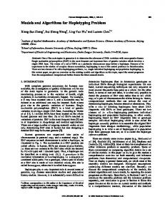
Figure 1.2: Time-space diagram for the tracks between Rotterdam and Utrecht. and long term planning purposes. In practice, most of the planning of operational timetables is still done manually. Figure 1.2 shows an example of one cycle time of a cyclic timetable in the form of a time-space diagram. The horizontal axis shows the stations that are passed on the route from Rotterdam on the left, to Utrecht on the right. The vertical axis shows the time, in this case for one cycle time of sixty minutes. The lines in the diagram show the various locations of trains on this track at a given point in time; the numbers correspond to particular trains. For example, consider train 21700 represented by the dashed lines. Within the displayed time frame this train travels once from Utrecht to Rotterdam, and back. At eight minutes past the hour it leaves Rotterdam, as can be seen in the lower left part of the diagram. The train arrives in Utrecht at forty-two minutes past the hour.

1.3.4

Platform and track assignment

Not all the infrastructure details are taken into account in the construction of the timetable. The exact routing of trains at junctions for example, or the routes through stations are not considered. In particular, the routing of the in-station traffic can be a complex problem (see Zwaneveld [88] and Zwaneveld et al. [89]). Here, the problem is to find routes for trains to pass through a station, given the layout of the station, and a timetable. Similar to the timetabling problem, there is a set of hard safety constraints on, for example, the train movements and the distances between trains. Additionally, the routing should retain as much of the service issues of the timetable

1.3. PLANNING PROBLEMS FOR PASSENGER RAILWAYS 0

10

20

7500

Ehv 3500

Ah

50

60

Asd

Zl

Ehv 3500

Ah

Zl 7500

Ah

Hdr

Gvc 2000 Nm

7a 7b

Hdr

2000 Nm

Gvc Rtd

3000 Nm

Es

Hlm 900 Mt

500

Rtd

Ah

Gvc

3000 Nm

Gn

Hlm

Rtd

Gvc Rtd 1700

Ehv

Asd

14000

8a 8b

Rhn Gvc

11a 11b

40

Zl 5600

4a 4b 5a 5b

30

Asd

Zl

7

2000

Koln100

Gn

500

Nm

Gvc

20

Rhn Es

1700

Nm

Hdr

900 Ehv

30

5900

Rtd Gvc

Hlm

3000Nm

10

Rhn

2000

Hdr

800 Mt

0

Rhn

Rtd Gvc

Hlm

12a 12b

5900

3000 Nm

40

50

60

Figure 1.3: An example of a platform assignment for the station Utrecht.

as possible, such as connections and preferred dwell times. The platform assignment of trains to platforms follows from the routes assigned to the trains. Figure 1.3 shows some of the available platforms at Utrecht along the left vertical axis, while the horizontal axis shows the times at which a platform is used. The lines in the figure indicate trains that are halting for specified periods of time at available platforms. The schematic station layout of the station Utrecht can be seen in Figure A.1 on page 133. We consider the platform and track assignment as a separate problem from the timetable construction. In practice, however, one is not considered without the other, and thus a timetable is also assumed to describe a platform and track assignment.

1.3.5

Rolling stock planning

Although the platform and track assignments take the infrastructure details into account, an accurate assignment of rolling stock to the train lines is not made. The type and quantity of the engines and carriages to be used, and the more detailed routing of these units is made in the rolling stock planning. The efficient use of the rolling stock is important, especially for commercially oriented railway operators, since it is one of their largest cost sources. The rolling stock planning can be divided into two phases. First, the total amount of available rolling stock is distributed over the operated train lines (see Abbink et al. [3]), without making a detailed circulation plan. Second, a detailed rolling stock circulation is constructed for every line, given the total number of units assigned to this line in the first phase (see Alfieri et al.

8

CHAPTER 1. INTRODUCTION

9:00 Gvc

9:30

10:00

10:30

173 1

533

173 5

537

21 73 1

20 53 3

21

20 53 7

11:00

11:30

173 9

12:00

541

5

39

17

17 34

20 54 1

7 53

53 2

21 73 9

3 17

3 53

9

31 17

52

4 52

5

73 0

Ut

73

52 8

Rtd

17 26

Ut

Amf

17 2

16 29

7

17 31

17

16 33

16 37

35

Dv

0

3 17

2

3 16

34 17

6 63

0 64

8 73

Es 9:00

9:30

10:00

10:30

11:00

11:30

12:00

Figure 1.4: An example of a rolling stock assignment.

[6], Schrijver [76] and Peeters and Kroon [67]). The circulation describes the routes of anonymous units of rolling stock. Which physical units will be used is not yet known. Current research in both assignment phases is directed to the handling of capacity shortages. If there does not exist a feasible assignment such that all passengers can be seated, then the overutilisation is minimised. Figure 1.4 shows an example of a rolling stock assignment for the train units operated on the railway tracks between Gvc (Den Haag) and Ut (Utrecht), Rtd (Rotterdam) and Utrecht, and Utrecht and Es (Enschede). This time-space diagram is similar to Figure 1.2, but with the space and time axes interchanged. Instead of showing the positions of trains, it shows the positions of rolling stock units. For readability, only the start and end segments of the diagonal lines are drawn. The line colours indicate the kind of rolling stock to be operated. Consider, for example, the two trains 1731 and 21731. Train 1731 leaves Den Haag a few minutes after 9:00 with three train units headed for station Utrecht, as shown in the upper left corner of Figure 1.4. Around the same time, train 21731 departs from Rotterdam, also with three units, and also heading towards Utrecht.

1.3. PLANNING PROBLEMS FOR PASSENGER RAILWAYS 05.00

06.00

Es 1616

07.00

08.00

Amf

Asd

1616

1625

Amf

Es 1616

1620

Es

1629

Amf

Asd

1620

1629

Amf 1620

10.00

Es

1624

15.00

16.00

17.00

1637

Shl

Amf 1628

Amf Hgl

Hgl 1641

Asd Amf

1632

1641

Es Hgl

1633

Hgl

1641

Amf 1640

Asd Amf 1633

Amf

1641

1629

Amf 1624

14.00

1629

Amf 1624

13.00

Hgl

Hgl

1633

Es

12.00

Amf

1637

Amf

Shl

1620

11.00

Shl

1624

Shl

1616

Es

09.00

Amf

9

Asd Amf

1640

Amf 1640

1640

Hgl

1649

Amf

Es 1644

Es

1649

Hgl

1649

Shl 1653

Amf

Hgl

1653

Figure 1.5: A Gannt chart with duties.

Both trains arrive in Utrecht at approximately 9:45. The three units of the 1731 train are coupled with two of the three units of the 21731 train. The combination continues as train 1731 to Dv (Deventer), where two units are decoupled and transferred to train 636. The coupling and decoupling of train units is also referred to as combining and splitting.

1.3.6

Crew scheduling

The journeys of the trains, also of the empty trains or equipment between stations, are split into sequences of trips. A trip is a segment of a train journey that must be serviced by the same crew, without rest periods. The problem of crew scheduling deals with the construction of duties from a given collection of trips. Each duty has to satisfy several constraints, such as a maximum length of 9:30 hours. An example of seven duties is given in Figure 1.5. The trips are represented by the boxes in the chart. The numbers in the boxes correspond to the trains of which the according trip is part. Due to the large number of trips—around 10,000 for some instances reported in Kroon and Fischetti [43]—and side constraints on the duties, practical crew scheduling problems are highly complex to solve. The general approach for making a crew schedule is, therefore, not based on the individual members of the workforce, but on these generic duties. The duties are later assigned to the actual crew members in the crew rostering phase. For more information on crew rostering and scheduling, see Caprara et al. [16] and Kroon and Fischetti [43]. It is clear that the crew scheduling/rostering problem and the earlier planning problems such as rolling stock planning are correlated. However, due to the complexity, these problems are mostly considered separately, although some researchers considers an integrated approach (see Freling [31], Freling et al. [32] and Wren and Fares Gualda [87]).

10

CHAPTER 1. INTRODUCTION Kampen

Zwolle

Amersfoort

Meppel Almelo

Deventer

Figure 1.6: An example of a station layout of the station Zwolle.

1.3.7

Shunting and maintenance planning

At the end of the planning process, after the timetable and rolling stock circulation are known, comes the problem of finding suitable shunting and maintenance plans. Let us first consider the shunting plan. During the rush hours, most of the rolling stock is in use. At other times of the day, and especially during the night, not all train units are needed, and, therefore, they have to be parked. The processes involved with moving the rolling stock units to and from their parked positions are called shunting, or dispatching (see Gallo and Di Miele [34], Winter and Zimmermann [86] and Freling et al. [33]). The shunting movements are restricted by the available railway infrastructure, and by time and safety constraints. The available shunt tracks are not all identical. While some can be approached from both sides, others must be called in a last-in, first-out fashion. This is especially a complicating factor if the rolling stock units are also not all identical. The shunting problem is not only the problem of matching incoming and outgoing rolling stock units, and parking them on available shunt tracks, but also to schedule the routing on the station infrastructure, and for cleaning and short term maintenance. For an example of the available tracks around a station—the station layout—see Figure 1.6. Maintenance planning is generally done when the rolling stock circulation is known. It considers the deviations from the circulation that are necessary to carry out the maintenance of the individual carriages. The rolling stock schedule, as discussed in §1.3.5, only contains information about anonymous units. Not only would a more detailed planning make the scheduling problem much more difficult to solve, but due to possible disturbances the location of rolling stock is uncertain long before the date of operation. Several days before the maintenance of units is due, their location is known and the operated detailed circulation is altered to allow these units to visit one of the available maintenance facilities in the network. This may have consequences for the shunting plans. For recent research on this topic, see Kroon et al. [44]. As mentioned before, the input/output relations between the problems described above are not as strictly sequential as shown in Figure 1.1. Through feedback loops in the overall planning process, the occurrence of a critical problem at one stage can

Local Planning

11

Evaluate Basic One-hour Timetable

1

Standard Week Plan

Daily Plan

(Year Planning)

(Day Planning)

Central Planning

1.4. THE OVERALL PLANNING PROCESS AT NSR

Basic One-hour Timetable

1

Standard Week Plan

(BOP/BPA)

2

Daily Plan

(Year Planning)

(Day Planning)

12 Months

2

9 Months

3

Operational control

(BOP/BPA)

3

8 Weeks

3 Days

Figure 1.7: The current planning process. call for a replanning at another, earlier stage. The overall planning process specifies the general structure and order in which the different problems are tackled. In the next section we review two overall planning processes: first with an emphasis on early detailed planning, and second a structure in which the planning of details is postponed as much as possible.

1.4

The overall planning process at NSR

The planning process at NSR can be divided into several chronological stages and into several organisational structures. Every stage deals with a subset of the planning problems of §1.3. Though possibly with some differences, the planning process at NSR exists also for other railway operators. Let us consider both the current planning process, and a conceptual planning process to be used in the near future.

1.4.1

Current planning stages

The current planning stages are schematically shown in Figure 1.7. These processes are described in detail in Prins [69] and Peeters [66]. The stages differ in two dimensions. First, the three stages are ordered chronologically, and differ moderately in the level of detail. Second, there is the distinction between how the chronological stages are treated by both the central and local planning departments. At the most abstract level in the planning process lies the construction of the basic one-hour timetable (BOT), consisting of the basic one-hour pattern (BOP), and the basic platform assignment (BPA). The BOP gives a cyclic one-hour time-space

12

CHAPTER 1. INTRODUCTION

diagram for every track in the network (see also §1.3.3). The BPA adds in-station details such as the platform assignments of the various trains in the BOT. The BOT is constructed centrally at NSR, but is checked at the different local planning departments. There is a feedback loop between the central and local planning departments to arrive at a feasible BOP and BPA. For railway operators such as NSR, that operate a cyclic timetable, this is the main step in the overall planning process. In order to complete the other planning stages, the BOP and BPA must be ready approximately nine months before the new timetable is scheduled to begin. At the next stage, the one-hour timetable is extended to a timetable for one standard week by the central planners. This stage takes roughly seven months, and ends a few months prior to operations. It incorporates most of the planning details. Both the rolling stock and crews are planned centrally (see also §1.3.5 and §1.3.6). In addition, the detailed shunting plans are constructed. These plans are tested locally for their feasibility. If changes to the standard week plan are necessary, then this is reported to the central planning department, which proposes modifications and restarts the feedback cycle. The standard week plans are adjusted several times per year, using so-called adjustment sheets5 . Ultimately, daily plans are constructed throughout the year to fill in the details of the standard week plan. For individual days of the year, the daily plans take into account the planned maintenance of the infrastructure, but also, for example, extra train services offered at large events such as soccer matches. Note that this also requires altering the timetable. The daily plans are designed in the same way as the standard week plan. Again, the central planners plan the rolling stock and crew, and the local planners test the feasibility of the necessary shunting operations. If the constructors of the daily plans identify structural problems in the standard week plan, then the standard week plan is adjusted by the central planners. As can be seen on the time line of Figure 1.7, most of the time is used at the second stage, the planning for one standard week. Due to the high level of detail in the standard week plan, the necessary correction cycles between central and local planners often take significant time. To reduce the overall makespan, NSR has launched a large-scale redesign project for the planning process. These proposals are discussed in the next section.

1.4.2

Proposed planning process

To identify possible capacity problems with the daily planning and scheduling, the original standard week plan of Figure 1.7 describes many details, such as the rolling stock schedules and the shunting plans. However, the share of these details that are critical for the feasibility of the standard week plan is only small. In addition, the usefulness of these details is limited in the construction of the daily plans. For example, due to maintenance of the infrastructure, the planned rolling stock schedules need to be altered, which in turn influence the shunting plans, etc. Thus, much of the time spent on making the detailed plans can be saved. The main goal for redesign is 5 In

Dutch Wijzigingsbladen

1.4. THE OVERALL PLANNING PROCESS AT NSR

13

Basic One-hour Timetable

Operational control

Process coordination

1 2 3 Basic Days

Specific Days

(BOP/BPA)

9 Months

3 Months

4 Weeks

3 Days

Figure 1.8: The new planning process concept.

to reduce the makespan of the planning process. The proposed planning process is described in Figure 1.8. Note the absence of separate local and central planning departments. By investing in information and communication technology, these planning departments are virtually integrated to decrease the time lag caused by feedback loops. Still, any request or demand for changes in the plans is coordinated between the involved planning stages. Similar to the first stage in Figure 1.7, the process starts with the construction of the BOT. Now, however, the planning of infrastructure details is advanced to this first phase, but only for so-called critical shunting and train activities. For a discussion on how to recognise a priori whether the required shunting movements for a train line will be critical, see Reinartz and Fassaert [73] and Van Eck van der Sluijs et al. [24]. Other preliminary studies, aimed at making rough capacity estimates, are also made for the rolling stock and crew plans. This causes the first planning stage to be longer than the original three months. At the second stage, the BOT is used to construct the complete timetable for a set of basic days. Although the planning for the basic days is comparable to the current planning of a standard week, the makespan is considerably shorter. This is achieved by delaying the planning of uncritical details. Especially by the elimination of several correcting feedback cycles between local and central planning, this could considerably shorten the lag times and thus the makespan. At the final stage, all the detailed plans for several weeks are made in parallel. These plans are made a number of weeks ahead of operation, using a rolling horizon. Thus, for example, in week 33, the new rolling stock circulation and crew schedule are made for the weeks 38-43, while in week 34 the planners are constructing the schedules for the weeks 39-44. This is represented in Figure 1.8 by the stacked Specific Days.

14

CHAPTER 1. INTRODUCTION 1

2

3

4

5

6

7

8

9

A

A

B

B

C

Westbourne Park

C

Hammersmith D

D

Gloucester Road E

E

F

F

2

3

4

5

6

7

8

9

Figure 1.9: Line plan of the underground system in London (see London Underground [49]).

1.5

An introduction to line planning

A line plan lies at the heart of almost all scheduled public transport, whether it concerns bus or subway systems, regular trains, high speed trains, or airline services. All of these line plans specify a list of operated services between pairs of locations that are operated at a given frequency. This frequency can range from several times per hour for subways, to bimonthly services for a stagecoach line from the mid eighteen hundreds. An example of a modern day line plan is given in Figure 1.9. The underground system in London dates back to 1863, when the world’s first underground railway opened. The fourteen lines in this system have all been given names, such as the Hammersmith & City Line, the Picadilly Line, and the Victoria Line. A line plan lies at the basis of the operated timetable. While for the stagecoach example at best a specific day was known, a timetable in general specifies the times at which the operated means of transport calls at a station. On the other hand, for a system with high frequency connections, such as the London Underground, a detailed timetable is—at least for the passengers—no longer necessary. Instead, the fastest way by underground for an example trip from Gloucester Road to Westbourne Park is described as “At Gloucester Road, wait for Picadilly Line train. At Hammersmith, wait for Hammersmith & City Line train. At Westbourne Park, arrival” (see Figure 1.10). For the public railway service in the Netherlands, a growing political interest in

1.6. RESEARCH OBJECTIVE From: GLOUCESTER ROAD To: WESTBOURNE PARK Station Duration Gloucester Road … Hammersmith 15 mins. … Westbourne Park 29 mins. Journey Duration:

15

Action Wait for PICCADILLY LINE train Wait for HAMMERSMITH & CITY LINE train Arrival

29 mins.

Figure 1.10: How to get from Gloucester Road to Westbourne Park (see London Underground [49]). spatial planning contributed in the 1970s to the introduction of a three train system of regional, interregional and intercity trains, and several new railway lines, such as the Schiphol line and the Flevo line (see NRC [57]). Further large-scale changes in the line plan and timetables were made in the beginning of 1998, when the frequencies of many intercity and interregional trains were increased. These changes turned the Dutch railway network into the busiest network in Europe. Recently, several large infrastructure projects have been put forward, such as the high-speed passenger lines HSL Zuid, HSL Oost and the Hanze line, but also freight lines such as the Betuwe line or the IJzeren Rijn line. The fate of some of these projects is not yet known. They were designed to increase the accessibility of the Randstad from the rest of northern Europe, and to and from the northern provinces of the Netherlands. On a smaller scale, though far from marginal, are infrastructural projects such as the Hemboog, and Gooiboog that offer shorter connections through new railway tracks. For more information, see ProRail [71]. The privatisation of NS also caused an opposing development. The reduced governmental interest for the operated services nearly resulted in the discontinuation of several unprofitable lines. However, in 1999, the Dutch Ministry of Traffic and NSR signed a performance contract6 that linked the right of NSR to be the single operator on the main part of the Dutch railway network, to a list of performance guarantees on their services. These guarantees covered both lower bounds on the punctuality of trains, and minimum operated frequencies between stations (see NRC [56]). As a result, the continuation of services on the unprofitable lines was ensured. This clarity also led to the founding of several regional operators, such as Syntus, Noordned, and Oostnet. Several unprofitable lines will be contracted by other operators in the near future.

1.6

Research objective

The aim of this thesis is to explore mathematical models and solution techniques for aiding the construction of railway line plans, with an emphasis on the efficient use of the available resources. This research topic is of high importance both for the service 6 In

Dutch Prestatiecontract

16

CHAPTER 1. INTRODUCTION

to the traveller, as well as for cost efficiency of the railway operator. The lag time of investments for expanding the railway infrastructure or the rolling stock is too long to handle the growing passenger demand in the short run. Therefore, to meet the service standards and the traveller’s growing mobility requirements, the currently available capacity must be used at high efficiency. This efficient use of resources is in line with the objectives of modern railway operators, as a consequence of the privatisation and the resulting competition on the tracks. The line plan holds a pinnacle position within the planning process of railway operators. Reasons for adding or altering lines in the existing system vary. For the customer, the addition of new lines can directly decrease the travel time. Additionally, increasing the line frequencies may be preferable since it increases the traveller’s planning freedom, and may reduce the expected travel time. The introduction of new lines can also reduce the system’s vulnerability to delays. As an example, consider introducing a combination of short lines to replace a geographically long train line. A delay in the service of a long line can easily propagate through the network, since the long route has many blocking opportunities for other train lines. For the railway operator, focussing on the design of the line plan is important for the efficient use of the available resources—both of the infrastructure, and of the rolling stock and personnel. Efficient use of the rolling stock, especially at times of capacity shortages, cuts both ways. It is not only of value to the operator, but also increases the service to the passengers. The efficient use of the infrastructure and personnel, even though not directly interesting for the customer, can influence the level of service through, for example, lower operating costs and thus lower ticket prices. The importance of research into the efficient use of resources, starting with line planning, has also been recognised by several independent studies, such as Project B&B [70], V&W [84] and NYFER [61]. For an overview of early literature on line planning, consider Bussieck [11]. The main objective in early work was to construct line plans that provide a high number of direct train connections for the travellers. A drawback of the direct travellers approach is that it often yields lines with geographically long routes. Besides the delay sensitivity of long lines mentioned before, there are also capacity related implications. A train line covering a geographically long route often has a significant variation in the number of passengers along its route. Depending on the available capacity, this leads to underutilisation or overutilisation, both of which are undesirable. After the first steps in the mid 1990s by the European Union to come to privately owned railway operators, the research trend has moved to cost efficiency objectives. This lead to publications such as Claessens et al. [18], Zwaneveld [88] and Bussieck [11]. Of course, focussing on minimising the operating costs can also have negative effects. The most important disadvantage is that it can go at the expense of the service to the customer, e.g., by causing an increase in the number of passenger transfers.

1.7. OUTLINE OF THIS THESIS

1.7

17

Outline of this thesis

This thesis is structured as follows. First, the two chapters of Part I address various foundations. Chapter 2 gives an introduction into combinatorial optimisation problems and techniques. Chapter 3, on the other hand, focusses on issues in line planning modelling. We address topics ranging from the estimation of demand data, to topics involved with the throughput capacity of the railway network. In the second part of this thesis we discuss three applications of mathematical models for railway line planning problems. In Chapter 4 we develop and analyse a branch-and-cut algorithm for solving cost-minimising line planning problems. We discuss new preprocessing techniques for these problems in §4.3, and also discuss a range of cutting plane classes and tree search issues such as branching rules and primal heuristics. Then, in §4.4, the implementational details of these techniques are discussed. For example, in §4.4.2 we describe the algorithms that are used to find violated cutting planes of the various classes that were introduced before. The proposed methods are then put to the test using a number of real-life line planning problems in §4.5. The line planning model of Chapter 4 considers a separate line planning problem for each of the different types of trains, such as regional trains and intercity trains. Chapter 5 introduces the multi-type line planning problem. We develop three model formulations for this problem in §5.3 using a simplified sub-problem called the edge capacity problem. Equivalence proofs for these formulations are given. Yet, their performance in solving practical instances differs significantly. This is tested in §5.4. The line planning models that were described in Chapter 4 and Chapter 5 design a new line plan. For every proposed line the halting stations are dictated by the type of the line, and the types of the stations along its route. However, these station types are part of the input of the line planning problem. Alternatively, Chapter 6 presents a model that reconsiders the stations at which the trains stop for a given line plan. This model is then used to determine the halting stations in such a way that the total travel time of passengers is minimised. First, in §6.2, we introduce new concepts, such as the line-event graph. Then, in §6.3 we show how to formulate this problem as a multi-commodity network flow problem with additional constraints and variables. Using Lagrangian relaxation, we show in §6.4 how to find lower bounds for this problem. To effectively use these bounds in a branch-and-bound framework, we introduce a number of preprocessing and tree search techniques, together with a problem-specific multiplier adjustment algorithm. This is discussed in §6.5. In §6.6 we, once again, describe a computational study based on instances of the Dutch passenger railway operator NSR.

Part I

Foundations

19

Chapter 2

Combinatorial foundations The results in the following chapters build on well-known foundations of combinatorial optimisation. In this chapter we recall the basics of such topics as (multicommodity) network flows, integer programming and branch-and-bound. In the discussion of these topics, some familiarity with the basic notation and definitions of graph theory is assumed. For a general introduction into combinatorial optimisation, see Nemhauser and Wolsey [55], Papadimitriou and Steiglitz [65] and Schrijver [75, 77].

2.1

Polyhedral combinatorial optimisation

This section gives a short introduction into the field of combinatorial optimisation, and in particular to polyhedral methods.

2.1.1

Combinatorial optimisation problems

A typical description of a combinatorial problem is given using a finite ground set E and a family F of subsets of E called the feasible sets. Now, given a cost ce for every element e of E, a combinatorial optimisation problem can in general be written as max

X

subject to F ∈ F

ce

(2.1)

e∈F

An example of a classical combinatorial optimisation problem is the maximum cardinality matching (MCM) problem: Given a graph with a set of vertices and edges connecting them, what is the largest subset of edges such that every vertex is part of at most one of the edges in this subset. For the MCM problem, an edge in the graph represents a matching between its two vertices. The ground set is built up out of all the edges, while the feasible sets consist of all feasible matchings. Since the MCM problem is concerned with finding the largest number of edges, all the weights of elements of the ground set are equal to one. A variation of this problem is the 21

22

CHAPTER 2. COMBINATORIAL FOUNDATIONS

(a) affine hull

(b) convex hull

Figure 2.1: Two types of hulls for the two points x1 = (1, 2) and x2 = (3, 1) from R2 . maximum weighted matching problem, where every edge is given a specific weight to indicate how valuable the edge is. A relaxation of a maximisation problem is a problem max cR (F )

subject to F ∈ FR

(2.2)

where the feasible set FR contains F, and for which every solution PF of the original problem yields at least the same objective function value, i.e., e∈F ce ≤ cR (F ). Even though maximisation problems are considered here, these ideas carry over to minimisation problems with only minor changes. For example, relaxations of maximisation problems yield upper bounds, while for minimisation problems, they result in lower bounds. We will refer to the objective function value of a relaxation as a dual bound , and call a feasible solution to the original problem a primal bound .

2.1.2

Polyhedral theory

Polyhedral theory links combinatorial optimisation to integer and linear programming, discussed in the next section. Therefore, let us first give a short theoretical introduction. Fundamental in polyhedral theory are the concepts of linear combinations and convex combinations. We denote the Euclidean linear space of dimension n by Rn . Consider a set of k > 0 points S = {x1 , . . . , xk } ⊆ Rn . Some point y ∈ Rn is called a linear combination of the points in S, if for Pk Pk some scalars λ1 , . . . , λk ∈ R it holds that y = i=1 λi xi . If it also holds that i=1 λi = 1, then y is called an affine combination of the points in S. An affine combination with λi ≥ 0 for all i ∈ 1, . . . , k is referred to as a convex combination. The set of convex (affine) combinations of all points of S is called its convex (affine) hull. The convex hull of some set S is often written as conv(S). See also the examples in Figure 2.1 for n = 2. A hyperplane in Rn is defined as the set of points {x ∈ Rn } that satisfy the nontrivial equation ax = b, where a ∈ Rn \ {0} and b ∈ R. Alternatively, the set {x ∈ Rn : ax ≤ b} is called a halfspace. A polyhedron is the intersection of a finite

2.1. POLYHEDRAL COMBINATORIAL OPTIMISATION

23

set of halfspaces. It is a well-known result in combinatorial theory that a bounded polyhedron in n-dimensional real space is structurally equivalent to the convex hull of a finite set of points in Rn (see Minkowski [51] and Weyl [85]). Therefore, not all the definitions of a polytope in the literature are the same; some define it as simply a bounded polyhedron, while others use the convex hull description. An inequality ax ≤ b is said to be valid for a set S ⊆ Rn if S ⊆ {x ∈ Rn : ax ≤ b}, i.e., if S is contained within the halfspace defined by ax ≤ b. Alternatively, a point x∗ ∈ Rn violates the inequality if ax∗ > b.

2.1.3

Integer linear programming problems

The link between combinatorial optimisation problems and polyhedra can be made, for example, by introducing variables xe that take the value 1 if e belongs to a feasible set F , and 0 otherwise. These variables thus describe a feasible set F ∈ F as a point in Rn , where n is the size of the ground set. Using these variables, the optimisation problem of (2.1) can also be described as X max ce xe subject to x ∈ S (2.3) e∈E

where the set S is defined as the union of all feasible incidence vectors ( 1 if e ∈ F F xe = 0 otherwise which make up the feasible set S = {xF ∈ Rn : F ∈ F}. If this set is not empty, then there always exists an optimal vertex solution to X max ce xe subject to x ∈ conv(S) (2.4) e∈E

that is also in S. Following the equivalence between polytopes and bounded polyhedra, there exists a finite set of inequalities for which the intersection of the defined halfspaces is equal to conv(S). Therefore, the optimisation problem given above can be solved using linear programming (LP) techniques. Finding the convex hull of a set of feasible solutions is, however, often not trivial, since the number of necessary linear constraints may be very large. The feasible sets of combinatorial optimisation problems are frequently defined using integer linear descriptions, such as S = {x ∈ Zn : Ax ≤ b}

(2.5)

where b is a vector, and A is a matrix of appropriate dimensions. Note that this integer linear description can easily be extended to also incorporate continuous variables. Consider again the maximum cardinality matching problem on a graph with m vertices and n edges. The constraints Ax ≤ b and x ∈ Zn must enforce that every

24

CHAPTER 2. COMBINATORIAL FOUNDATIONS

vector x ∈ Rn that satisfies them is an incidence vector of a matching, and vice versa. This can be achieved by using Ax ≤ b to enforce that every vertex is incident to at most one of the edges in the matching: X xe ≤ 1 for all vertices v. (2.6) e∈E:v∈e

Combined with the integrality restriction x ∈ Zn , the restrictions 0 ≤ xe ≤ 1

for all edges e

(2.7)

complete the integer programming formulation of the feasible set of MCM. For proving the correctness of this integer programming formulation, first consider a feasible matching F , and the solution xe = 1 if e ∈ F , and xe = 0 otherwise. Clearly, since every vertex is part of at most one edge, the first class of constraints is satisfied. By construction the solution is integer and all xe are between 0 and 1. Second, consider a feasible integer solution xe . From 0 ≤ xe ≤ 1 it follows that xe ∈ {0, 1}. By contradiction, if the solution F = {e ∈ E : xe = 1} is not a feasible matching, then apparently there exists a vertex v that is part of two edges e and e0 in the matching F . This, in turn, implies xe = xe0 = 1, and thus that the constraint of the class (2.6) for vertex v is violated, since it has a left-hand side value of at least 2. The vector x can therefore not be a feasible solution, which contradicts our initial assumption.

2.1.4

Solution approaches

There are no known methods for solving general integer linear programming problems efficiently. Moreover, many core combinatorial problems, including general integer linear programming, belong to the class of N P-hard problems (see Garey and Johnson [35]). For this class of problems it is strongly believed that no algorithm exists with a worst-case running time that is bounded by a polynomial in the size of the input. Cutting plane method For linear programming problems, on the other hand, there exist polynomial time algorithms. A well-known property of linear programs is that for every problem that is defined over a bounded polyhedron and for which an optimal solution exists, there also exists an optimal solution that is a vertex of the associated polyhedron. Consider solving the linear programming relaxation of (2.3) for S defined as in (2.5) X max ce xe subject to x ∈ PLP , e∈E

where PLP = {x ∈ Rn : Ax ≤ b}. In case this linear program results in an optimal solution that is integer, then this solution is also optimal for the problem defined on (2.5) since S ⊆ PLP . Notably, if conv(S) = PLP , then every optimal solution to

2.1. POLYHEDRAL COMBINATORIAL OPTIMISATION

25

3x1 + 4x2 £ 5

x1 + x2 £ 1 Figure 2.2: The feasible points, their convex hull, and the LP polytope. the LP relaxation is also feasible, and thus optimal for the original problem on S. However, in general the convex hull of S and the LP relaxation polytope are not equal. This is illustrated in the following example. Consider the feasible region in Figure 2.2. The feasible set S is defined as S = {x ∈ Z2 : 0 ≤ x1 ≤ 1, 0 ≤ x2 ≤ 1, 3x1 + 4x2 ≤ 5}, or equivalently, S = {(0, 0), (1, 0), (0, 1)}. Since the convex hull of S is strictly contained within the LP polytope PLP = {x ∈ R2 : 0 ≤ x1 ≤ 1, 0 ≤ x2 ≤ 1, 3x1 + 4x2 ≤ 5}, the LP relaxation can yield solutions that are not part of conv(S). However, consider the inequality x1 + x2 ≤ 1. This restriction is valid for conv(S), because conv(S) is contained in the halfspace defined by this inequality, i.e., x1 + x2 ≤ 1 is satisfied by all solutions of S. Yet, adding this constraint to the problem formulation will cut off part of the original PLP polytope. Therefore, it is also referred to as a cutting plane, i.e., a valid inequality ax ≤ b for which PLP * {x ∈ Rn : ax ≤ b}. Adding x1 + x2 ≤ 1 to the description of the problem makes the linear programming relaxation coincide with conv(S). Thus, the original problem can be solved using this new linear programming relaxation. This method is also known as the cutting plane method. It was first introduced by Dantzig et al. [20], and is outlined below. (1) Given are a feasible set S = {x ∈ Zn : Ax ≤ b} and its linear programming relaxation PLP = {x ∈ Rn : Ax ≤ b} (2) Solve the LP relaxation, and let x∗ be the optimal solution. (3) If x∗ ∈ S, then x∗ is optimal for S. Hence, stop. (4) Otherwise, identify a cutting plane ax ≤ b that is violated by x∗ . (5) Add the inequality to PLP , and goto step (2). Step (4) is the most important step of the method. The problem of identifying whether a solution x∗ is feasible, or else to find a violated valid inequality—a cutting

26

CHAPTER 2. COMBINATORIAL FOUNDATIONS

plane—is also known as the separation problem. Gr¨otschel et al. [40] showed that in general, the separation problem is polynomially solvable if and only if the original optimisation problem is polynomially solvable. Note, however, that this does not exclude the existence of polynomial time separation algorithms for specific classes of valid inequalities. Over the last decades, many classes of valid inequalities, and separation algorithms have been found for a wide range of combinatorial problems (see Nemhauser and Wolsey [55] and Aardal and Van Hoesel [1]). We also refer to §4.3.2 and §4.4.2 for classes of cutting planes and separation algorithms specifically for line planning problems. For the maximum cardinality matching problem, Edmonds [25] showed that the two classes of inequalities given before, together with the class of odd-set constraints   X |U | xe ≤ for all odd-sized subsets U ⊆ E 2 e∈E(U )

describe the complete convex hull of matchings. Even though there is an exponential number of odd-set inequalities, the separation problem can be solved in polynomial time (see Padberg and Rao [64]). This is in line with the existence of a polynomial time combinatorial algorithm for MCM described in Edmonds [26]. In general, however, the cutting plane method can fail in step (4), ending with a solution that is not in S, e.g., a solution that is fractional. In such cases, an enumerative algorithm such as branch-and-bound can be used. Branch-and-bound-and-cut The classical principal of branch-and-bound is best described as divide and conquer. The principle is that, if optimising over S is too difficult, perhaps the problem can be solved by optimising over subsets of S, and then taking the best of these solutions. For the MCM problem, for example, the set S can be split into two subproblems S|xe =0 and S|xe =1 for some edge e. Obviously, this division can also be done recursively, e.g., for various edges. The subproblems are also called the nodes of the branch-and-bound enumeration tree. To prevent complete enumeration, a dual bound is computed at every node of the branch-and-bound tree. The value of this relaxation is a bound on the best solution of the subproblem associated with the current node. At this point, there are four possible outcomes: (1) The relaxation is infeasible. (2) The optimal solution to the relaxation is feasible for the original problem. (3) The optimal solution to the relaxation is worse than the best-known primal bound. (4) None of the above. Clearly, the value of a feasible solution for the original problem is a primal bound on its optimal value. Throughout the search process, the best feasible solution is

2.1. POLYHEDRAL COMBINATORIAL OPTIMISATION

27

stored in memory. In the first three cases, further investigation of the current node can be stopped. Otherwise, the problem at the current node is split into subproblems for new child nodes. All the nodes are stored in a list of active nodes. When a node has been evaluated, it is removed from this list. Thus, as soon as the list of active nodes is empty, the original problem is solved. In most branch-and-bound implementations, the dual bound on the subproblems is calculated by solving the LP relaxation. In addition, to implement the branch-andbound algorithm, we have to solve the problem of how to select the next subproblem (node selection strategy), and how to create new subproblems (branching rule). For a comprehensive study of these topics, see Linderoth and Savelsbergh [47]. We also refer to §4.3.3 and §6.5.3 for specific node selection and branching rules for line planning problems. As can be seen, the quality of the derived bounds influences the size of the enumeration tree. The integration of the cutting plane method in the branch-and-bound algorithm is an obvious next step. In early work, the branch-and-bound algorithm was used after no more cutting planes could be found by the cutting plane algorithm. This is also called cut-and-branch. The alternative is to apply the cutting plane algorithm at every branch-and-bound node to improve the value of the LP relaxation. This is referred to as branch-and-cut. Several branch-and-cut software libraries have been developed in recent years. For a short overview, see Lad´anyi et al. [46]. Lagrangian relaxation The idea to use a relaxation of the original problem to obtain a dual bound on the objective value can be taken further than the linear programming relaxation. The observation that relaxing some of the constraints, e.g., the integrality restrictions, makes the underlying problem easier to solve, is also used in a technique called Lagrangian relaxation (LR). For two classical studies of the use of Lagrangian relaxation for integer programming, see Geoffrion [36] and Fisher [29]. In addition, Ahuja et al. [5] gives a good overview of the Lagrangian relaxation technique, and several applications in network optimisation. As an example, consider the integer linear problem IP zIP = max cx s.t. A1 x ≤ b1 2

A x≤b x ∈ Zn+ .

2

(complicating constraints) (nice special structure)

where n = m1 +m2 , and m1 and m2 are the number of rows of A1 and A2 respectively. For notational purposes, let us combine the integrality restrictions and the class of nice constraints in the feasible set Q = {x ∈ Zn+ : A2 x ≤ b2 }. The idea is now that the problem of optimising solely over Q is much easier to solve than IP. Therefore, by dualising the complicating constraints, we obtain a problem that is easier to solve, and whose optimal value is a dual bound on the optimal value of the original problem. This is explained in the next paragraphs.

28

CHAPTER 2. COMBINATORIAL FOUNDATIONS

For the problem IP, as defined above, the Lagrangian relaxation LR(λ) for any 1 vector λ ∈ Rm + , is defined as zLR (λ) = max cx + λ(b1 − A1 x) s.t. x ∈ Q. The complicating constraints A1 x ≤ b1 are not part of the feasible set Q. These constraints have been replaced by a penalty term λ(b1 −A1 x) in the objective function. Thus, since the element λi for every relaxed constraint i in 1, . . . , m1 is nonnegative, any violation of these constraints A1 x ≤ b1 worsens the objective function value. The vector λ is referred to as the vector of Lagrangian multipliers. 1 The Lagrangian relaxation LR(λ) is a relaxation of IP for any λ ∈ Rm + . Any feasible solution x of IP clearly satisfies x ∈ Q, and is therefore also feasible for LR(λ). For the objective function value of LR(λ) it is easy to see that cx + λ(b1 − A1 x) ≥ cx holds for any feasible solution x of IP, since λ ≥ 0 and A1 x ≤ b1 . Thus, zLR (λ) ≥ zIP for any λ ≥ 0. The Lagrangian dual problem LD is the problem of finding the vector λ that results in the tightest (lowest) upper bound, i.e., zLD = minλ∈Rm 1 zLR (λ). +

(2.8)

The vector of multipliers at which this minimum is attained, is denoted by λ∗ . There are several reasons for considering Lagrangian relaxation techniques. A first reason is found in the following theorem. Theorem 2.1. If, for a given vector λ, the solution vector x satisfies the three conditions 1. x is optimal for LR(λ) 2. A1 x ≤ b1 3. λ(b1 − A1 x) = 0 then the vector x is also optimal for the original problem IP. If only the last condition is not satisfied, then x is at most  away from the optimal solution of IP, with  = λ(A1 x − b1 ). These are the well-known conditions under which a solution of a Lagrangian relaxation is also optimal for IP (see Geoffrion [36]). The condition λ(b1 −A1 x) = 0 is also called the complementary slackness condition. Note that, since all elements of λ are nonnegative, these conditions thus state that for every element i ∈ {1, . . . , m1 } either λi is zero, or (b1 − A1 x)i is zero (or both). Also note that  is nonnegative, since the solution vector x satisfies A1 x ≤ b1 by the second assumption. The optimality conditions given in Theorem 2.1 show that Lagrangian relaxation is not only useful for obtaining dual bounds, but may also yield optimal solutions to the underlying problem IP.

2.2. MULTI-COMMODITY FLOWS

29

Another reason for considering Lagrangian relaxation is the quality of the Lagrangian dual, as compared to the linear programming relaxation of IP. As was shown in Geoffrion [36] zLP ≤ zLD (2.9) for a general maximisation problem like IP, where zLP is the optimal value of the linear programming relaxation of IP. In other words, the optimal Lagrangian bound LR(λ∗ ) is at least as good as the bound obtained from the linear programming relaxation. However, Geoffrion [36] also gives conditions under which the two bounds are equal. This is stated in Nemhauser and Wolsey [55] as follows. Theorem 2.2. If all the extreme points of {x ∈ Rn+ : A2 x ≤ b2 } are integral, then zLP = zLD for any cost vector c. Thus, under the mentioned conditions, the Lagrangian bound is not better than the LP bound. In such cases, it can still be preferable to use Lagrangian relaxation for dual bounding, if the Lagrangian bound is easier to compute (see also §6.4). So far, we have not considered the problem of optimising the Lagrangian dual in (2.8). It is essential that for a given vector λ, the problem structure of the relaxed problem LR(λ) is easy to solve. Now, first observe that zLR (λ) is piecewise linear and convex (see, for example, Geoffrion [36] and Nemhauser and Wolsey [55]). The methods used to solve the problems of the Lagrangian dual can be divided into two categories. The most widely used methods use subgradient optimisation algorithms. Even though many versions of such algorithms exist, the property that is used is that for some vector λ and the according optimal solution x ¯ of LR(λ), the vector b1 − A1 x ¯ is a subgradient of zLR at λ. The idea in these algorithms is that the optimal vector λ∗ for LD can be found by sequentially updating λ ← λ + s(b1 − A1 x) with a decreasing step size s. For examples of generic subgradient optimisation algorithms, see Ahuja et al. [5], Bazaraa et al. [8] and Nemhauser and Wolsey [55]. Alternatives to subgradient optimisation are multiplier adjustment methods. Here, the combinatorial structure of the particular problem is used to find the optimal multiplier vector. Several examples in the literature are known where this method outperforms generic subgradient based algorithms. Fisher [29] presents a small overview and some empirical data for these methods. For an example of multiplier adjustment methods for the generalised assignment problem, see Fisher et al. [30]. In Volgenant and Jonker [81], a detailed description is given of adjustment techniques for the symmetric travelling salesman problem, based on the 1-tree relaxation. Again, more information on Lagrangian relaxation can be found in §6.4.

2.2

Multi-commodity flows

A basic problem in the class of network flow problems is the minimum cost (“mincost”) flow problem. For an in-depth coverage of network flow problems, see Ahuja et al. [5]. In min-cost flow problems, the question is how to transport a commodity through a network as cheaply as possible, while satisfying demand at certain nodes

30

CHAPTER 2. COMBINATORIAL FOUNDATIONS

from available supplies at other nodes. Most instances also take into account the limited availability of capacity on the links (arcs) between the nodes. Consider a directed graph D = (V, A) with vertices V , and directed arcs A connecting the vertices. The demand or supply at a vertex i ∈ V is given by b(i). The quantity b(i) is also called the net supply of vertex i. If b(i) is negative, then b(i) is considered a demand vertex, whereas b(i) > 0 implies that i is a supply vertex. On every arc (i, j) between two vertices i and j, an upper bound uij and lower bound lij is given on the total amount of flow across arc (i, j). Now, given a cost cij per unit of flow for all arcs (i, j) ∈ A, the min-cost flow problem can be formulated as X min cij xij (2.10a) (i,j)∈A

s.t.

X j:(i,j)∈A

X

xij −

xji = b(i)

for all i ∈ V

(2.10b)

for all (i, j) ∈ A

(2.10c)

j:(j,i)∈A

lij ≤ xij ≤ uij

where a variable xij represents the amount of flow on an arc (i, j). The objective function (2.10a) sums up the total cost of the flow vector x. The constraints (2.10b) are referred to as the mass balance constraints. These restrictions enforce that for every node i, the total flow leaving i, minus the total flow entering i, is equal to the net supply of i. For example, for nodes with a net supply of zero, i.e., with b(i) = 0, the constraints (2.10b) ensure that the total amount of inflow equals the total amount of outflow. Very often, these restrictions are also stated in matrix notation as N x = b, where N is the node-arc incidence matrix, and x and b represent the flow vector and net supply vector. The constraints (2.10c) reflect the lower and upper bounds on the amount of flow on the arc from i to j. The min-cost flow problem is well-known to be polynomially solvable. This accounts for why, as was mentioned in §2.1.4, Lagrangian relaxation techniques have many applications in network optimisation. One of the properties of min-cost flow problems is the integrality property: If all arc capacities, supplies, and demands of nodes are integer, then there always exists an integer minimum cost flow, if the instance is feasible. If there is only one vertex i with b(i) > 0, then the problem is called a single source problem. Observation 2.3. The single source min-cost flow problem without capacity restrictions can be solved by finding a shortest path tree rooted at the source vertex. Because the problem is uncapacitated, every unit of flow that is sent from the source vertex s to some target vertex t can follow a shortest (cheapest) path through the network. Multi-commodity flow (MCF) problems arise when several distinct commodities use the same underlying network. The ways in which the commodities differ can be, e.g., their physical characteristics, or simply their origin and destination in the network. Since they use the same network, the commodities compete for the available capacity on the arcs. These capacity restrictions bind the commodities together.

2.3. THEORETICAL OVERVIEW

31

For an MCF problem, let xkij and ckij denote, respectively, the amount of flow of commodity k on arc (i, j), and its cost per unit. Similar to the linear programming formulation of the single-commodity flow problem, the MCF problem can be formulated as X min ck xk k

s.t. N xk = bk X xkij ≤ uij

for all (i, j) ∈ A

k

where xk and ck are the flow vector and per unit cost vectors. Note that the objective function allows for different costs per arc for units of different commodities. The restrictions in N xk = bk are the mass balance constraints for every commodity. The second class introduces for every arc (i, j) in the network an upper bound uij on the total flow of all commodities using (i, j). If the flows through the network are allowed to take non-integral values, then the min-cost multi-commodity flow problem is polynomially equivalent to linear programming, and thus solvable in polynomial time (see Itai [42] and Gr¨otschel et al. [40]). However, the integrality property of single-commodity flows does not hold for multi-commodity flows. The MCF problem with integral flows is N P-hard, even in the case of only two commodities (see Even et al. [28]). Observation 2.4. If there are no capacity restrictions on the arcs in an MCF problem, then the MCF problem can be solved by considering a separate single-commodity flow problem for every commodity. This observation is also used in the application of Lagrangian relaxation to MCF problems. By dualising the capacity restrictions, the LR problem for a given value of the multiplier vector λ does not involve capacity restrictions and can thus be solved efficiently. For a complete example, see Ahuja et al. [5].

2.3

Theoretical overview

The techniques and models discussed in the previous sections are used in various chapters throughout this manuscript. Chapter 4 presents an integer programming formulation for modelling the line planning problem. For this formulation, we describe in detail a branch-and-cut algorithm. This includes several new classes of cutting planes, and accompanying separation techniques. Using a set of practical instances, it is shown that the use of branch-and-cut for this problem can yield optimal, or at least very good, primal and dual bounds in short time. The results in Chapter 5 depend to a large extent on multi-commodity flow models. By considering passengers as commodities that want to be transported through the railway network, an MCF model is used to prove the validity of a number of alternative formulations by showing their equivalence. These (mixed) integer linear formulations, presented in §5.3.2 and §5.3.3, are used for solving three real-life instances.

32

CHAPTER 2. COMBINATORIAL FOUNDATIONS

Chapter 6 combines multi-commodity flow models with the theory of Lagrangian relaxation. The problem at hand is modelled as an MCF problem with additional restrictions. However, for real-world instances, the resulting problems are too large to handle. Therefore, using Lagrangian relaxation techniques on the additional constraints, the overall problem is split into a series of subproblems that can each be solved efficiently.

Chapter 3

Foundations in line planning modelling This chapter bridges the gap between the real-world environment described in the introduction, and the models discussed in the next chapters. Here, we focus on practical aspects of line planning, and on how they are modelled, or left out. This chapter also introduces the notation and mathematical concepts that are specific for the railway models presented in later chapters.

3.1

Line plans and cyclic timetables

The line planning problem, as presented in §1.5, is concerned with determining on which routes to operate trains, and at what hourly frequencies. This definition implies the construction of cyclic timetables. Such timetables are repeated, more or less identically, every hour of the day (see also Peeters [66] and §1.3.3). The passenger demands, however, vary significantly throughout the different hours of the day. The morning and afternoon rush hours, for example, are the busiest parts of the day (more on this topic in §3.3.3). The alternative, an a-cyclic timetable, offers more opportunities to the railway operator to fine-tune the timetable to match these demand fluctuations. Such a line plan could contain many trains during the rush hours, but only few trains during the rest of the day. A line plan and cyclic timetable can only adapt to the fluctuating market demand by adjusting the operated capacity of the train lines. Typically, during rush hours, high capacity trains are used, such as longer and/or double-deck trains. In off-peak hours, trains may consist of less carriages. In practise, a hybrid concept is possible, based on a cyclic core timetable. This allows extra trains to be operated during rush hours that are not available during low-traffic hours. However, the amount of available infrastructure and rolling stock is often a binding factor in railway services during peak hours. 33

34

3.2

CHAPTER 3. FOUNDATIONS IN LINE PLANNING MODELLING

Rolling stock

The main cost factors that determine the operating costs of a line plan are the costs of using the infrastructure, and the costs of the required personnel and rolling stock. Both the number of trains needed to operate the lines at given frequencies, as well as the necessary number of conductors and drivers, depend on the circulation of the rolling stock, and therefore on the timetable. For this reason, some authors consider an integrated approach to construct a timetable and a rolling stock circulation (see Nachtigall [52, 53] and Lindner [48]). However, neither the timetable, nor the rolling stock circulation are known when the line plan is constructed. Therefore, to estimate the amount of necessary rolling stock, we assume a circulation schedule in which all rolling stock is dedicated to specific lines. So, the switching of rolling stock between lines is kept to a minimum, and thus the interdependencies among the train lines are reduced (see also the reliability issues in §1.2.1). We assume that every train line is operated in both directions. This is standard policy for most railway operators, since it offers a more transparent service to the passenger. We also suppose that the composition of rolling stock units of trains is the same in each direction. In addition, the trains used to operate a single line are assumed to be identical, i.e., pulling the same number of carriages. Now, given the line’s hourly frequency and the number of carriages per train, the costs of operating a specific line can be determined using the circulation time (see also §3.5.3). Splitting and combining of trains during their trips is assumed to be not allowed. In practise this splitting and combining is sometimes done for two lines that have a significant part of their route in common: two trains can be combined at the station where their routes meet, and split where the trains leave the common route. An example of this is given in §1.3.5. Although the splitting and combining of trains may have a negative impact on the punctuality, it also allows for more direct connections for passengers. At the same time, the capacity on the tracks taken up by the combined trains is less than for the two separate trains. This is, for example, due to minimum safety distances between trains (see also Peeters [66]). Other restrictions are not due to the availability of the rolling stock, but because of the rolling stock itself. In particular, consider the combining of train units to build trains. The train units of NSR are classified according to classes and subclasses1 . Figure 3.1 shows units of three different classes, and for every class two subclasses. The class Koploper consists of two subclasses: a subclass with three carriages called Koploper 3, and a subclass with four carriages referred to as Koploper 4. Such units cannot be split into smaller parts. Trains can only consist of units of one class, although possibly of different subclasses. For example, a Koploper train combines units of 3 and 4 carriages. As a consequence, it is not possible to make a Koploper train with 5 carriages in total. Similarly, the Regiorunner class has units of 4 and 6 carriages, while the Mat’64 class can combine units of 2 and 4 carriages. In general, all these train units can move in two directions by themselves, and, thus, do not need 1 To avoid confusion with the types that are used to define the halting patterns of lines, we do not use the common types and subtypes here.

3.3. PASSENGER DEMAND

35

additional locomotives. Note that the bottleneck for the maximum number of rolling stock units of a train is often the platform length of the visited stations, rather than the physical and technical limitations of the units.

3.3

Passenger demand

In this section, we discuss passenger demand and service to the passengers in connection with line planning. The topic of estimating the demand was already briefly discussed in §1.3.1. We also address issues concerning cost-oriented line planning and the service to passengers, as mentioned before in §1.6. Most railway operators offer their travellers a number of differently priced comfort alternatives. Similar to airline companies, two such levels are often used: first class and second class. As mentioned by NS [59], next to short travel times, passengers value a high level of service and comfort. By offering, e.g., more comfortable seats in much less crowded carriages, a modest percentage of the travellers is willing to pay around 60% more, compared to the price of a second class ticket (see NS [60]). With insufficient train capacity, some travellers—often those who travel second class— question whether the two-class system should remain. Throughout this thesis we do not make a distinction between classes, and consider only aggregated data. This is, however, merely a strategic modelling decision.

3.3.1

Passenger demand and capacity planning

There are many different alternatives for representing the passenger demand. Consider, for example, cross-section data. In railway transport terms, the cross-section data describes the numbers of passengers in the trains that run in parallel at a particular moment in time. In the time-space diagram of Figure 1.2 on page 6, the lines in the figure mark the positions of trains at different points in time. This time-space diagram describes the basic one-hour timetable for a specific part of the network, but in general such a schedule is available for a complete day, and for every part of the network. Now, the trains in the eight o’clock cross-section, for example, are those trains that cross the imaginary horizontal line of eight o’clock. Cross-section data is often used in the allocation of rolling stock. It is clear that, at least from a service perspective, the number of units that is assigned to every train in the timetable must meet the demand of passengers as well as possible at every moment of the day—in particular for the 8 a.m. cross-section (see Abbink et al. [3]). This is an example of bottleneck planning, since the morning rush-hour is usually the busiest time of the day. More on the variation of demand over time can be found in §3.3.3. The problem with using cross-section data for line planning is obvious: the data is defined on an existing set of lines, and thus not suitable for designing a new line plan. An example of a method that can describe the passenger demand without using a line plan or timetable, is the origin-destination (OD) matrix. The rows and columns of this matrix represent the different stations in the network. Thus, a cell

CHAPTER 3. FOUNDATIONS IN LINE PLANNING MODELLING 36

(a) Koploper 3 (ICM-1, ICM-2)

(b) Koploper 4 (ICM-3, ICM-4)

(c) Regiorunner 4 (VIRM-IV)

(d) Regiorunner 6 (VIRM-VI)

(e) Mat’64 2 (Plan V)

(f) Mat’64 4 (Plan T2)

Figure 3.1: Different types of rolling stock (Pijpers [68]).

3.3. PASSENGER DEMAND

37

of the matrix refers to a particular OD pair, and contains the total number of people that, within a given time period, want to make this trip. The problem of estimating OD matrices, for example as part of overall traffic modelling, has received a lot of attention in the last fifty years (see, e.g., Abrahamsson [4], Bierlaire [9] and Sherali and Park [79]). The OD matrix, in general, refers to the number of trips between any two geographic locations. The splitting of all trips over the available travel modes, such as car, bus, train, underground or on foot, is called a modal split. An example of an origin-destination matrix between a set of railway stations is shown in Figure 3.2. The origin stations are given on the vertical axis. The size of the bubble for a pair of stations (v, w) represents the number of travellers from v to w, within a period of one hour. Train travellers often have a number of combinations of train lines and connections available to take them from their origin to their destination. These connections may even involve several geographically different routes. As mentioned before, a passenger’s choice is influenced by the different travel times, ticket prices, necessary train changes, and comfort and service levels. The problem of estimating how users travel through the network is known as the traffic assignment problem. The traffic assignment problem is another important step in the analyses of transportation demand, besides the estimation of the OD matrix (see Safwat and Magnanti [74]). A traffic assignment simulation model specific for railway systems is described by Oltrogge [63]. In order to make capacity assignments to lines in a proposed line plan, we have to be able to estimate, or to make assumptions on, how passengers will traverse the network and which train lines they will take. Since finding such a traffic assignment is not trivial, we make assumptions on the route choices of passengers through the network. One possibility is to let the line planning model determine a traffic assignment, that is ideal for minimising the operating costs of the line plan. Since the model thus dictates the trips of passengers, this solution can be far from the true traffic assignment made by passengers themselves. In particular, it can involve excessively large travel times for certain travellers, if this would have a positive effect on the total amount of assigned capacity. A first alternative is to assume an a priori assignment of passengers to geographical routes through the network. From the passenger’s perspective, this is comparable to the restrictions enforced by the ticket regulations. The freedom of the line planning model is now restricted to assigning the passengers to train lines along the prescribed route. This assumption has two important implications. Firstly, it can be used to exclude unrealistic traffic assignments in which some travellers are expected to use unnecessarily long routes. Secondly, this assumption on the routes of passengers can be used to simplify the line planning models considerably (see Chapter 5). The prescribed routes could be the shortest routes in the network, or the observed routes taken by travellers according to the currently operated timetable. The essence is that the route is known for every traveller. The above approach is used in the models that are presented in Chapter 4 and Chapter 5. The capacity that is allocated to the lines of the new line plan must suffice to transport all passengers. The difference in the assumptions in this respect,

38

CHAPTER 3. FOUNDATIONS IN LINE PLANNING MODELLING

Rsd

Etn Bd Gz Tbwt Tb Ht Hto Rs Ow O Rvs Wc Nmd Nm Est Ah Ahp Ahpr Vp Rh Dr Bmn Zp Dv Ost Wh Zl

Rsd

Etn Bd Gz Tbwt Tb Ht Hto Rs Ow O Rvs Wc Nmd Nm Est Ah Ahp Ahpr Vp Rh Dr Bmn Zp Dv Ost Wh Zl

Figure 3.2: An example origin-destination matrix.

3.3. PASSENGER DEMAND

39

between Chapter 4 and Chapter 5, is that in the former we assume that the traffic assignment has been split into assignments for the different train systems, such as intercity trains and regional trains. Such a system split is used by many authors (see Bussieck et al. [12], Claessens et al. [18]). Another alternative is the traffic assignment model used in Chapter 6. Here we use, e.g., estimates of the amount of time needed to change from one train to the next to predict the shortest path of passengers with respect to travel time. Different from the first traffic assignment, this assignment therefore depends on the operated line plan. Such an assignment model can be used since Chapter 6 is involved with determining halting patterns of trains given a line plan. This model is then used in §6.6 for an analysis of the line plans that were proposed in Chapter 5. The problem with all these approaches is clear: the assumed traffic assignment— split or not—and the OD matrix need not be realistic when the new line plan is put into operation. The newly-determined line plan can in turn influence the behaviour of potential travellers. For example, a line plan that offers more frequent and direct connections between stations might well encourage travellers currently using their car to switch to using the train. For a more detailed discussion on the substitution effect between public transportation and car travel, see V&W [82, 83]. The approach applied in practice is to evaluate the resulting line plan using detailed traffic assignment models. The resulting demand data is used to generate a new line plan, and so on, hopefully obtaining a consistent passenger allocation within a small number of iterations.

3.3.2

Passenger demand across the network

The concern of §1.6 is that a line plan that aims to minimise the operating costs could have a negative impact on the service to the customer, if the new line plan results in an increase in the travel times or the necessary number of train changes. This effect depends on the structure of the passenger demand across the network. If, for example, the length of the trip of a passenger is small compared to the lengths of the tracks in the network, then the number of necessary train changes will also be low. An example distribution of the trip lengths of passengers is visualised in Figure 3.3. This figure is based on morning rush-hour data from NSR. The recorded distances are the lengths of the shortest paths in the railway network. As mentioned in §1.1, the average trip length in the Dutch network is around 35–40 kilometers, while nearly 50% of the passengers travel less than 25 kilometers. However, the average distance between consecutive intercity stations is 27.3 kilometers, and 19.0 and 6.5 kilometers between interregional and regional stations respectively.

3.3.3

Passenger demand variations over time

The passenger demand varies over time from one hour to the next, and from day to day. This behaviour is illustrated in Figure 3.4, which shows the total number of travellers in the system at different points in time. The distribution peaks at the morning rush hour around eight o’clock and in the afternoon at roughly half past

40

CHAPTER 3. FOUNDATIONS IN LINE PLANNING MODELLING 100%

15%

90% 80%

12%

% of travellers

70% 60%

9% %Cum.

50%

%Trav.

40%

6%

30% 20%

3%

10% 0%

0% 0

10

20

30

40

50

60

70

80

90

100

Travelled distance (km)

Figure 3.3: The (cumulative) percentage of travellers grouped by travel distance. Distance group 0 includes all trips with a length of [0, 5) kilometers, etc. five. The morning rush hour is generally busier, while the evening rush hour is spread over a larger time interval. The trips in the evening are often the return trips of the morning journeys. The line plan is by definition a plan for one standard hour. Thus, we assume that the OD matrix on which the line plan is based portrays a steady state situation. An alternative would be to determine a core line plan, including a subset of lines that are not operated in off-peak hours, similar to the hybrid timetable concept discussed in §3.1.

3.4

Infrastructure

In this section we discuss issues in line planning related to the stations and the tracks in the network.

3.4.1

Station capacity

The number of trains a station can handle per hour depends, among other things, on the available platforms and the lengths of the platforms, the possible simultaneous routes through the station, and the available tracks and crew for shunting movements. Every train that visits a station, whether it halts there or passes through without stopping, occupies the tracks and platforms at that station for a certain amount of time. The necessary amount of time depends on the type of the train and on the type of rolling stock. Turning a train around can take, e.g., between 10 and 30 minutes.

3.4. INFRASTRUCTURE

41

100%

Percentage of peak flow

90% 80% 70% 60% 50%

%Trav.

40% 30% 20% 10% 2:00

0:00

22:00

20:00

18:00

16:00

14:00

12:00

10:00

8:00

6:00

4:00

0%

Time

Figure 3.4: The number of travellers at different points in time. In addition, there are also service aspects, such as a preference for cross-platform connections, that influence the utilisation of platforms. The number of routes through a station can, in a similar way, be a binding factor in the throughput capacity of a station (see also §1.3.4). Another important restrictive factor is concerned with the parking of train units and related processes, i.e., the shunting. As mentioned in §1.3.7, the shunting of trains is restricted by the available railway infrastructure, available personnel, and by time and safety constraints. When more and more trains visit a station, any of these three factors can become critical in the operational process. Therefore, the station utilisation is an important factor in the investigation of how to increase the throughput capacity of the railway network.

3.4.2

Homogenising the train system

As mentioned in §1.2.2, several recent studies propose a homogenisation of the train system to create more throughput capacity on the railway network (see NS [59], Railforum [72] and Project B&B [70]). There are several approaches for doing so, as shown in Figure 3.5. The current timetable is shown in Figure 3.5(a). There are two lines being operated: an intercity line departing every 15 minutes from station a and going directly to station g, and a regional line, stopping at every station, and also leaving a every 15 minutes, but three minutes after the intercity line. Given that the trains have no opportunity to pass each other on the tracks and that there must always be a minimum distance of three minutes between subsequent trains, the maximum number of connections between a and g in this instance is 8 connections

42

CHAPTER 3. FOUNDATIONS IN LINE PLANNING MODELLING

per hour. A first alternative approach considers shortening the lengths of the train lines. An example is shown in Figure 3.5(b). By splitting the regional line into three separate lines, and letting one depart before the feeder line arrives, the travel times of the two original lines become more homogenous. Therefore, the throughput capacity can increase. This option would, however, be inconvenient for the travellers that enter and leave the system in the regional stations. These passengers have to change trains more often. Another option, debated in NS [59], Railforum [72] and Project B&B [70], is to abandon the strict hierarchical pattern of ordered station and line types. Figure 3.5(c) demonstrates the effect of introducing a system where one line halts at a, c, e and g, and the other at a, b, d, f and g. Similar to the first approach, this also homogenises the travel times of both lines, thereby creating the possibility to stack the lines closer together in the timetable. Again, the number of lines per hour can increase. As a third approach, consider clustering the intercity trains and regional trains. This option is discussed in Peeters [66]. By homogenising the traffic order and velocity, a higher number of connections per hour can be achieved. However, this setting is not likely to be implemented, since it is not attractive for travellers. A last option—that requires additional investments—is the building of new tracks to increase the possibilities for faster trains to overtake slower ones. This alternative is visualised in Figure 3.5(e). By using a combination of building new tracks for overtaking, and by relaxing the halting patterns, NS [59], Railforum [72] and Project B&B [70] conclude that the throughput capacity can be increased by roughly 30% to 40%. However, this would be achieved at the expense of an increase in the delay sensitivity of the timetable. This is also emphasised in NYFER [61].

3.4.3

New railway safety systems

Supported by the European Commission, a new European railway traffic management system (ERTMS) has been designed to increase the track capacity, and to improve the safety and the interoperability between railway operators internationally. This system consists of two parts: the European Train Control System (ETCS) and the Global System for Mobile communications - Railways (GSM-R). ETCS is the new automatic control system for which the communication requirements, including voice and data communication, are provided by GSM-R (see ERTMS [27]). The ETCS includes a new train safety system by means of moving safety blocks. The current safety system, called a fixed block system, divides every track into a number of fixed blocks (see Figure 3.6). If, for example, one block is occupied by a train, then any oncoming train is given a red signal before entering this block, or even one block before. The sizes of the blocks are such that even the longest and heaviest train can stop within one block. With the new moving block system that is part of ETCS, these fixed blocks are replaced by safety blocks that move with the trains. The sizes of such blocks are based on the individual speeds, sizes and breaking powers of the trains. Using the

3.4. INFRASTRUCTURE

43

12:00

12:00

12:00

11:50

11:50

11:50

11:40

11:40

11:40

11:30

11:30

11:30

11:20

11:20

11:20

11:10

11:10

11:10

11:00

11:00

11:00 a

b

c

d

e

f

a

g

(a) Current situation

b

c

d

f

e

a

g

(b) Shorter lines

12:00

12:00

11:50

11:50

11:40

11:40

11:30

11:30

11:20

11:20

11:10

11:10

11:00

b

c

d

e

f

g

(c) Altered stops

11:00 a

b

c

d

e

f

(d) Clustered order

g

a

b

c

d

e

f

g

(e) Extra overtaking

Figure 3.5: The current situation with alternating intercity and regional trains (left), and four proposed modifications.

44

CHAPTER 3. FOUNDATIONS IN LINE PLANNING MODELLING

Red

Green

Yellow

40 kph

Red

Green

140 kph

Figure 3.6: The current situation with fixed safety blocks (top) and the moving block safety system (bottom).

GSM-R system, the drivers of the trains can now be given specific information on how to alter their driving speeds. Thus, the moving block system can allow trains to drive closer together, thereby increasing the throughput capacity of the infrastructure.

3.5 3.5.1

Modelling the railway system Infrastructure

The railway infrastructure of the stations and tracks is modelled as an undirected graph G = (V, E) of stations (vertices) and tracks (edges). This graph is also called the network graph. Every track e = {v, w} ∈ E, by definition represents the track connecting stations v and w of V . As an example, two network graphs are shown in Figure 3.7.

3.5.2

Lines

A line is described by a path in the railway network along which trains are operated at a given hourly frequency (see §1.3.2). The route that a line l follows through the network graph is given by a simple path of edges. For ease of notation, we define this route simply as l ⊆ E. The line planning problems discussed here are all based on selecting a set of operated lines from a large set of candidates. Therefore, an important part of the input consists of the set of candidate lines. Not every route between a pair of stations is a feasible candidate. Many infrastructural and operational restrictions have to be taken into account, such as the shunting possibilities for turning at the end stations and the maximum distance covered by a line. For every feasible pair of end stations, at most three possible connecting paths, i.e., candidate lines, are considered. These paths are, in general, the three shortest paths for the combination of begin and end

3.5. MODELLING THE RAILWAY SYSTEM

Figure 3.7: The Dutch and German (Bussieck [11]) railway networks.

45

46

CHAPTER 3. FOUNDATIONS IN LINE PLANNING MODELLING

60' 15'

15'

60' 135'

120'

105'

90'

75'

135'

0'

15'

30'

45'

60'

0'

(a) Once per hour

120'

105'

90'

75'

15'

30'

45'

60'

(b) Twice per hour

Figure 3.8: Trains versus frequency. station, where the length of the longest of these paths is not allowed to be more than twice the length of the shortest (see also Claessens et al. [18], H¨arte [41]). The stations at which a line stops, also called the line’s halts or dwells, are given by the type of the line. This type comes from a set of types T = {1, . . . , Tmax }. Not only is every line l associated with a type t(l), also every station v ∈ V is of a type tv from T . The halting pattern of l, i.e., the stations at which l halts, are defined by the line type t(l), and the types of the stations along the line’s route. The types often reflect the sizes of the stations: type 1 for stations in villages, up to type Tmax for stations serving large metropolitan areas. Most real-life railway instances consider three types of stations and lines. These are referred to as regional (R) for type 1, interregional (IR) for type 2, and intercity (IC) for type 3. Note that some authors refer to regional lines and stations as “aggloregional”. As is common in the Netherlands, but also in most other countries, the halting patterns of train lines follow a simple ordering. Train lines of type 1 halt at all stations they pass. Lines of type 2 skip the small stations of type 1, but halt at all stations of type 2 and higher, etc. Throughout this thesis we assume that the halting stations of lines follow this strict hierarchical pattern in which a line of type t halts at all stations along its route that are of type t, or higher. In practise, however, exceptions are sometimes made (see §3.4.2).

3.5.3

Rolling stock

It takes a number of trains to operate a line at a given frequency. To estimate the necessary number of trains without a timetable or a rolling stock schedule, we use the total time needed to operate the line in both directions and the time needed at both end stations to prepare the train for the reverse journey. Consider a line with a travel time of 60 minutes from the line’s origin to its destination station, as shown in Figure 3.8. At either end station, at least 15 minutes are needed to prepare the train for the reverse journey. This amounts to a total circulation time of 150 minutes. If the line is operated once per hour, this would require (at least) d150/60e = 3 trains (Figure 3.8(a)). However, operating the line at a frequency of two (Figure 3.8(b)), departing every 30 minutes, will call for d150/30e = 5 trains. In general, we let cpl denote the fractional number of necessary trains per

3.5. MODELLING THE RAILWAY SYSTEM

47

hour for some line l. The rolling stock is one of the largest cost drivers of a railway operator. The hourly costs of operating a line plan can be described by a function of fixed and variable costs per used train and per carriage (see also Claessens et al. [18]). The fixed costs are incurred for the availability of the individual trains and carriages and involve, for example, depreciation costs and fixed maintenance costs. Examples of variable costs per kilometer are cost sources such as ticket collectors costs, energy costs and maintenance costs. Now, the total cost of operating a line l at frequency f , and with c carriages per train can be calculated as tr car tr car dcpl · f e · (wfix + c · wfix ) + d · f · (wvar + c · wvar ).

(3.1)

This formulation thus incorporates four classes of resource costs: tr wfix

the hourly costs per train.

car wfix

the hourly costs per carriage.

tr wvar

the hourly costs per train per kilometer.

car wvar

the hourly costs per carriage per kilometer.

The distance in kilometers covered by l is given by the parameter d. Note that the total number of kilometers that is progressed in one hour by the trains of a line does not depend on the number of trains, but only on the frequency f and the distance d. To estimate the required amount of rolling stock and the involved costs, the line planning models of Chapter 4 and Chapter 5 not only decide on which lines to operate, and at what frequency, but they also assign a number of rolling stock units to every train line. The costs described above are for a period of one hour. As mentioned, this planning period is often taken to be the morning rush-hour, the busiest part of the day. However, the costs of one hour at peak-time are not representative for the costs at other hours, or at different days. Therefore, as proposed by Claessens [17], scaled estimates are used that reflect the total annual cost of operating a train for one hour during rush-hour. This concludes this introduction chapter on the railway related issues. The next part of this thesis considers three line planning applications.

Part II

Applications

49

Chapter 4

A branch-and-cut approach for solving railway line planning problems This chapter considers the problem of determining a cost-optimal line plan for a single train type. We present an integer linear programming model, and solve it using branch-and-cut. For this, we give a variety of valid inequalities and reduction methods. A computational study of five real-life problems based on instances of NSR is included. The results in this chapter are based on Goossens et al. [38].

4.1

Introduction

Traditionally, the objective when constructing a line plan has been to find a set of lines that maximises the number of direct travellers, i.e., the number of travellers that do not have to change trains during their journey (see also §1.6). This is an obvious target from a customer service point of view. However, it ignores important issues, such as the involved operating costs and the efficient use of the rolling stock. As an alternative objective, similar to Claessens et al. [18] and Bussieck [11], this chapter focusses on the problem of minimising the operating costs of a line plan. There are several approaches for formulating the cost-optimising line planning problem (CLP). In Claessens et al. [18], an integer nonlinear programming model is presented as a natural model for CLP. They transform this model into a linear programming problem on binary variables (BLP), and attempt to solve it using branch-and-bound. In Bussieck [11], an alternative formulation using general integer variables (ILP) is presented. In recent work, Bussieck et al. [13] reconsider the original nonlinear model. They study a relaxation of the nonlinear formulation to obtain good primal solutions of the original problem. Besides presenting the ILP formulation, Bussieck [11] also compares the BLP and ILP formulations using a cutting plane algorithm with cut-and-branch. He concludes 51

52

CHAPTER 4. BRANCH-AND-CUT FOR LINE PLANNING PROBLEMS

that the more compact ILP formulation is preferable for generating good feasible solutions. However, the lower bounds provided by BLP are superior to the lower bounds of ILP, therefore the BLP formulation is more suitable for proving optimality of a feasible solution. By extending the known reduction methods and classes of cutting planes presented, this chapter shows that the BLP formulation can be used to solve large instances of the problem using branch-and-cut, or at least to obtain excellent upper bounds and lower bounds in reasonable time. The model formulation is presented in the next section, recalling some of the details about line planning from Chapter 3. In §4.3 we describes the solution methodology. The implementational issues are described in §4.4. Finally, §4.5 presents a computational study based on instances of the Dutch passenger railway operator NSR.

4.2

Model formulation

A line specifies a route between an origin and a destination station and the subsequent stops, combined with the operated hourly frequency. The line plan is the set of operated lines. It does not incorporate any timetable information for the operated lines, though we assume that the timetable is cyclic with a cycle time of one hour, i.e., that the line plan is repeated every hour. This reflects the situation in the Netherlands, as well as in many other European countries. The model described here focusses on finding a line plan that minimises the induced operating costs, given the railway infrastructure with the accompanying stations and the number of travellers between stations. For a given network graph G = (V, E), as defined in §3.5.1, the travellers determine their route through the network based on the associated travel time. In general, this implies that they prefer to switch to lines of higher types at the earliest opportunity. As described in Oltrogge [63], this idea can be used to decompose the overall problem into separate line planning problems for the different types. Throughout this chapter, we therefore assume that the line planning problem considers exactly one type of lines. Such a system split is used by many authors (consider Bussieck et al. [12] and Claessens et al. [18]). Line planning models with multiple line and station types are discussed in Chapter 5. For an instance of type t, the network graph can be simplified in a straightforward way by removing all the stations at which lines of type t do not halt. The edges in G are modified accordingly. For an example, consider Figure 4.1. As discussed in §3.3, the demand data for the line planning problem are given by an OD matrix for which the route through the network is known for every traveller. Moreover, we assume that the flow of passengers is symmetric. Therefore, for every edge we can calculate the number of passengers traversing it. As a service to the passengers, we assume that each line is always operated in both directions. Thus, as in Claessens et al. [18], we can regard lines as being undirected. The level of service that the proposed line plan offers to the passenger is ensured by two conditions. The capacities of the lines should suffice to transport all passengers, and the line plan is enforced to guarantee a high number of connections between

4.2. MODEL FORMULATION

53

Figure 4.1: The Dutch network, and the network graph for the according IC instance (SP97IC).

every pair of consecutive stations in the network. We consider this issue in more detail in the next section.

4.2.1

Formulation

Our formulation of CLP is similar to the formulation used by Claessens et al. [18], and later in Bussieck [11]. Given is the undirected network graph G = (V, E) with vertex set V , edges E and a set of potential lines L. Every line l ∈ L corresponds to a set of edges that make up a simple path between the end vertices of l. The consecutive stops of line l are given by the stations corresponding to the vertices along its path, i.e., the stations v for which there is an edge {v, w} ∈ l. Recall that we consider only line planning problems with exactly one type of lines. For every line we have to decide whether to deploy it, and, if so, at what hourly frequency and with how many carriages. The set of possible frequencies for the lines is denoted by F ⊂ N, the possible number of carriages by C ⊂ N. As mentioned before, the resulting line plan must meet two types of service restrictions. For every edge e in the network, we are given a minimum number f e of passing trains per hour, and a necessary number of carriages he needed to meet the demand of all passengers who want to traverse e per hour. For formulating the line planning problem as an integer linear programming problem, we introduce a binary variable for every (l, f, c) ∈ N , with the set of triples as N = L × F × C. Every i ∈ N is used for referring to a particular (li , fi , ci ) combination. For convenience, we also introduce the set N (e) ⊆ N for every edge e as N (e) = {i ∈ N : e ∈ li }. The line planning problem CLP can now be formulated

54

CHAPTER 4. BRANCH-AND-CUT FOR LINE PLANNING PROBLEMS

as follows. zCLP = min

X

wi xi

(4.1a)

i∈N

s.t.

X

fi xi ≥ f e

for all e ∈ E

(4.1b)

fi ci xi ≥ he

for all e ∈ E

(4.1c)

for all l ∈ L

(4.1d)

for all i ∈ N

(4.1e)

i∈N (e)

X i∈N (e)

X

xi ≤ 1

i∈N |li =l

xi ∈ {0, 1}

where the decision variables xi for i = (li , fi , ci ) ∈ N are used to model ( 1 if line li is operated at frequency fi , with ci carriages per train xi = 0 otherwise The objective function coefficients wi represent the costs of operating the line associated with variable xi , as discussed in more detail in equation (3.1) in §3.5. The constraints (4.1b) enforce the minimum number of passing trains per hour on every edge e ∈ E. Restrictions (4.1c) impose the lower bound he on the number of carriages crossing edge e in one hour. Typically, he is the smallest number of carriages necessary for transporting all passengers across edge e. Note again that we consider all units of rolling stock to be identical. The third group of constraints ensures that every line is operated in at most one configuration. Contrary to Claessens et al. [18] and Bussieck [11], we have no upper bound restriction on the number of passing trains per hour for every track. Including these restrictions to account for possible bottlenecks in the infrastructure would be part of a more operational study. Claessens et al. [18] prove that finding a cost-optimal allocation of trains using only capacity restrictions is N P-hard. Since in general, that problem is a special case of CLP, it follows that CLP is also N P-hard. Before describing our branch-and-cut method, we first introduce some general notation and visualisation of CLP instances throughout the remainder of this chapter. Consider Figure 4.2. The instance consists of three stations, V = {u, v, w}, and two tracks, E = {e = {u, v}, f = {v, w}}. The pairs of numbers in brackets above the edges show the frequency and capacity lower bounds f e and he respectively. The overall set of candidate lines L for this network consists of three lines L = {l1 , l2 , l3 }. We refer to an individual variable xi as being of line li with a frequency of fi trains per hour, consisting of ci carriages, and therefore with an hourly capacity of fi · ci carriages.

4.3

Branch-and-cut method for CLP

The branch-and-cut techniques are divided into three sections: preprocessing (§4.3.1), cutting planes (§4.3.2) and tree search (§4.3.3). The preprocessing section focusses

4.3. BRANCH-AND-CUT METHOD FOR CLP

55

l1 l2 u

(f e,h e)

e = {u,v}

v

(2,7)

f = {v,w}

l3 w

Figure 4.2: Example of a CLP instance. on reducing the initial size of the problem. This is done by removing superfluous variables and constraints, and by tightening the model restrictions. Next, we discuss a variety of classes of cutting planes, both generally applicable, and cutting planes specifically derived for CLP. Finally, the tree search section covers branching rules and primal heuristics.

4.3.1

Preprocessing

The preprocessing techniques described in this section are designed to strengthen the initial formulation of the problem. Strengthening, in this context, covers both coefficient reduction techniques, and methods for reducing the number of variables and constraints used to model a given CLP instance. Claessens et al. [18] and Bussieck [11] describe several preprocessing techniques, specifically for CLP. We briefly recall these techniques and then review them in a more general context. Coefficient reduction The main constraints of the model—the capacity constraints (4.1c) and the frequency constraints (4.1b)—are strengthened using the methods described below. The coefficient strengthening or reduction techniques used here are extensions of ideas and techniques described in Dietrich and Escudero [21]. The coefficient strengthening techniques are described using a generalised line planning problem GLP with only two types of constraints. X zGLP = min wi xi subject to x ∈ S. (4.2) i∈N

The feasible set S is defined as all x for which Ax ≥ b Cx ≤ 1 x ∈ {0, 1}n

(4.3) (4.4) (4.5)

where N is the set of variables with n = |N |. The matrix A is an m × n matrix with nonnegative integer entries aij , and b is an m-dimensional vector of positive integers. Every variable xi is P associated with a unique line l ∈ L, denoted li . For every l ∈ L, there is a constraint i|li =l xi ≤ 1 in the second constraint matrix C. Note that CLP is contained in this class, where the constraints (4.3) contain the service constraints on the tracks.

56

CHAPTER 4. BRANCH-AND-CUT FOR LINE PLANNING PROBLEMS

We derive several methods for strengthening problems of this form. Using notation similar to Dietrich and Escudero [21], the coefficient akj of row k and column j can in general be strengthened to a ¯kj ← max{0, akj − ∆kj } = max{0, bk − Qkj }

(4.6)

where ∆kj = akj −bk +Qkj ≥ 0. Here, Qkj represents a lower bound on the left-hand side value of constraint k in any feasible solution x ¯ ∈ S with x ¯j = 1. To maintain the nonnegativity property for akj , we have added the lower bound on a ¯kj . Note that an initial strengthening can be obtained by setting a ¯kj = bk for all akj ≥ bk since we have assumed akj ≥ 0 and all variables are binary. This reasoning also implies Qkj ≥ 0. Next, we present two techniques for determining valid values for Qkj . Both techniques use an additional row from the constraint matrix A to strengthen its ˆ kj ≤ Qkj is valid. coefficients. Note that if Qkj is valid for S, then also any Q Alternatively, for any valid, though non-integer Qkj , it follows that also dQkj e is valid. Both techniques give lower bounds for the value of the following minimisation problem. Theorem 4.1. Consider an instance of GLP as defined by (4.2)-(4.5). Strengthening the coefficient akj of the constraint matrix A according to (4.6) with X X Qkj (h) = min aki xi subject to ahj + ahi xi ≥ bh , Cx ≤ 1, x ∈ {0, 1}n i6=j

i|li 6=lj

(4.7) if ahj < bh , and Qkj (h) = 0 otherwise, is valid for S for any constraint h. P Proof. We prove that for all x ∈ S it holds that (bk − Qkj (h))xj + i6=j aki xi ≥ bk . This is obviously true for all x ∈ S for which xj = 0, since then the new coefficientPof xj is unimportant. For all x ∈ S for which xj = 1 we have to show that i6=j aki xP i ≥ bk − (bk − Qkj (h)) = Qkj P(h). Clearly, any x ∈ S with xj = 1 satisfies ahj + i|i6=j ahi xi ≥ bh and xj + i6=j|li =lj xi ≤ 1, making x a feasible solution to the minimisation problem in (4.7). Solving the integer covering problem in (4.7) is in general too complex to use it for coefficient strengthening. We discuss two relaxations of this problem that give good bounds for Qkj (h). Example 4.2. Consider the set S of integer points x ∈ {0, 1}5 for which 3x1 + 4x2 + 7x3 + 4x4 + 6x5 ≥ 7 x1 + x2 + x3 + x4 + 2x5 ≥ 2 x1 + x2 + x3 ≤1 x4 + x5 ≤ 1 . Consider strengthening the coefficient of x3 in the first constraint. Although it is equal to the right-hand side, any feasible solution x ∈ S with x3 = 1 must still

4.3. BRANCH-AND-CUT METHOD FOR CLP

57

have at least one of the variables x4 or x5 set to 1 for the second constraint to be satisfied. Meeting the second constraint would therefore imply an additional left-hand side of Q13 = min{4, 6} = 4 units in the first constraint and therefore 3x1 + 4x2 + (7 − 4)x3 + 4x4 + 6x5 ≥ 7 is valid for S. Note that for instance the fractional solution {0, 0, 14 , 0, 87 } to the LP relaxation of S is cut off by the strengthened constraint. The following corollary generalises the idea of the previous example. Corollary 4.3. Consider an instance of GLP as defined by (4.2)-(4.5). Take two not necessarily distinct rows from the constraint matrix A, say rows h and k. Strengthening the coefficient akj according to (4.6) with ( akr if ahj < bh , 0 Qkj (h) = (4.8) 0 otherwise where r = argmini|li 6=lj ,ahi >0 aki , is valid for S. Proof. We prove the validity of Q0kj (h) by showing that it is the solution P to a relaxation of the optimisation problem in (4.7). Given that ahj < bh , then i|li 6=lj ahi xi > 0 is a relaxation of the restriction in (4.7). Now, for binary x, this new constraint is satisfied only if at least one xi with li 6= lj and ahi > 0 has value 1, and thus X X ahi xi > 0, x ∈ {0, 1}n . akr = min aki xi subject to i|li 6=lj

i6=j

Note that rows h and k need not be different. This method for finding valid Qkj works well on constraints with moderately sized bh − ahj . If this number is larger, we may consider another relaxation of (4.7), where we drop the integrality constraints imposed on the variables in the covering problem. As described later, the resulting continuous covering problem can be solved to optimality using a greedy algorithm. Example 4.4. Consider the feasible set S as introduced in Example 4.2. We again strengthen the coefficient of x3 in the first constraint. In any feasible solution x with x3 = 1, equation (4.7) tells us that strengthening a13 with Q13 = min 4x4 + 6x5

subject to x4 + 2x5 ≥ 1, x4 + x5 ≤ 1, x4 , x5 ∈ {0, 1}

is valid for S. If we drop the integrality restrictions on x4 and x5 , we can solve the remaining problem using a greedy algorithm. The optimal solution is x4 = 0, x5 = 0.5, which shows us that Q13 ≥ 3. From this it follows that 3x1 + 4x2 + (7 − 3)x3 + 4x4 + 6x5 ≥ 7 is valid for S.

58

CHAPTER 4. BRANCH-AND-CUT FOR LINE PLANNING PROBLEMS The following corollary generalises this idea.

Corollary 4.5. Consider GLP, taking two rows from the constraint matrix A, say rows h and k. Strengthening the coefficient akj of column j in row k according to (4.6) is valid for S, with X X Q00kj (h) = min aki xi subject to ahj + ahi xi ≥ bh , Cx ≤ 1, x ∈ [0, 1]n (4.9) i|li 6=lj

i6=j

if ahj < bh , and Q00kj (h) = 0 otherwise. Proof. Clearly, (4.9) is a relaxation of the optimisation problem in Theorem 4.1 and thus Q00kj (h) ≤ Qkj (h). The continuous covering problem with non-overlapping constraints (4.4) is closely related to the multiple-choice knapsack problem (see Martello and Toth [50]). It can be solved using a greedy algorithm similar to the one for continuous knapsack problems. Consider finding the optimal solution to min

n X

wi yi

subject to

i=1

n X

ai yi ≥ b, Cy ≤ 1, y ∈ [0, 1]n

i=1

in which w, a ∈ Zn+ and b ∈ Z+ . The constraint matrix C describes the nonoverlapping group constraints of (4.4) over all y variables. Without loss of generality, assume the variables are ordered so that w1 /a1 ≤ . . . ≤ wn /an . Now construct an optimal solution y ∗ as follows. Consider all variables in the given order, starting at y1 , and skip the P variable yj if it is in the same group as an already selected variable. Otherwise, if iakj

+

X

aki xi .

i|li 6=lj

Since the inequality (4.11) is valid for the original problem, it is also possible to recursively apply this technique for a set of variables. Note that the resulting inequality is order independent as long as at most one variable per line is used for probing, since the new coefficient ajk = 0. 2-Cover cuts This class of cutting planes, called 2-cover (2C) cuts, is based on the covering constraints in the CLP for a given track e. If variable xi alone does not satisfy both service constraints, then every feasible solution with xi = 1 will contain at least one more line across e. This observation is made in the following example. Example 4.13. Consider the following polytope S of a CLP instance S = {x ∈ {0, 1}5 : x1 + x2 + x3 + 2x4 + 2x5 ≥ 3}. Since at least two of these variables have a nonzero value in any feasible solution x1 + x2 + x3 + x4 + x5 ≥ 2 is valid for S. Lemma 4.14. Let the set C and its complement C¯ be defined as C¯ = {{i ∈ N (e)|fi ≥ f e , fi ci ≥ he } ¯ For any instance of CLP, the inequality and C = N (e) \ C. X X xi + 2xi ≥ 2 i∈C

(4.12)

¯ i∈C

is a valid inequality for every e ∈ E. Proof. Clearly, every feasible solution x ¯ for which x ¯i = 1 for i ∈ C¯ satisfies (4.12). ¯ by definition there must exist Alternatively, for any solution with x ¯i = 0 for all C, at least two distinct variables i, j in C with x ¯i = x ¯j = 1 for x ¯ to be feasible.

4.3. BRANCH-AND-CUT METHOD FOR CLP

63

The next corollary describes an extension of Lemma 4.14 in which the variables are divided into two or more parts. In particular, the resulting so-called multi-cover (MC) cuts consider n + 1 subsets. Corollary 4.15. Consider an arbitrary instance of CLP. Given a track e, and a positive integer n for which 2 ≤ n + 1 < he , then the inequality n X X s=1 i∈C s

sxi +

X

(n + 1)xi ≥ n + 1

(4.13)

¯ i∈C

is valid for CLP,Swith C s and C¯ given as C s = {i ∈ N (e)|he (s − 1) ≤ fi ci n < he s}, and C¯ = N (e) \ s C s . Proof. First, let us denote fi ci by ai and he by b. Note that all numbers are integers. Thus, si = min{s ∈ N|b(s − 1) ≤ ai n < bs} is equal to si = min{s ∈ N|(b − )(s − 1) < ai n < (b − )s} for suitably small  > 0. To prove that (4.13) is valid, we show that it is a Gomory cut (see Dietrich and Escudero [21]) obtained from (4.1c) with multiplication factor n/(b − ). This is clear for the left-hand side coefficients. It remains to be shown that dbn/(b − )e = n + 1 for all applicable values of b and n. Clearly, dnb/(b − )e ≥ n + 1. It is also easy to show that dnb/(b − )e ≤ dnb/(b − 1)e ≤ n + 1: dnb/(b − 1)e − (n + 1) = dnb/(b − 1) − (n + 1)e ≤ dn/(b − 1)e − 1 ≤ 1 − 1 = 0. Example 4.16. Consider the following polytope S of a CLP instance. S = {x ∈ {0, 1}5 : 3x1 + 5x2 + 7x3 + 10x4 + 14x5 ≥ 14}. If we consider n = 2, then C 1 = {1, 2}, C 2 = {3, 4} and C¯ = {5}, and thus from Corollary 4.15 it follows that the inequality x1 + x2 + 2x3 + 2x4 + 3x5 ≥ 3 is valid for S. Flow cover cuts The flow cover (FC) cuts are described in Bussieck [11]. These cuts use the line structure of CLP, in which lines typically cover more than one track. Example 4.17. Consider the CLP instance shown in Figure 4.4. Assume x ˜ is the optimal solution to the LP relaxation. If we divide the three tracks into two sets, e.g., {e0 } and C = {e1 , e2 }, then we can distinguish two types of feasible solutions: those containing at least one line using only e0 , and those in which all lines passing e0 also pass some tracks of C. Thus, either a valid line plan contains a line that uses only e0 , or validity implies that there are at least he0 carriages per hour being pulled along the tracks of C. Conversely, if we extend all lines passing some tracks of P C to also pass e0 , then lines that only pass e0 merely fill the gap between he0 and e∈C he . Since this is

64

CHAPTER 4. BRANCH-AND-CUT FOR LINE PLANNING PROBLEMS i

(li , fi , ci )

x ˜i

1 2 3 4

(l1 , 1, 6) (l2 , 1, 7) (l3 , 1, 12) (l4 , 1, 3)

1.0 1.0 0.5 0.34

l1

l2

d

l3

e0

e

(f e , he )

e0 e1 e2

(2, 19) (1, 7) (1, 8)

b

e1

e2

a

c l4 (19 − 7 − 8)˜ x3 + 1 · 6˜ x1 + 1 · 7˜ x2 + 2 · 3˜ x4 = 2 + 6 + 7 + 2 = 17 < 19 Figure 4.4: Example of a flow cover. a relaxation of the original problem, any valid inequality for this relaxation is also valid for the original problem. Therefore, we can reduce P the capacity coefficients of variables xi using e0 and not C from fi ci to he0 − e∈C he , or in this instance, to (19 − 7 − 8) = 4. P Lemma 4.18. Let C ⊂ E, e0 ∈ E \C for which he0 > e∈C he . Then, the inequality X X X X (he0 − he ) xi + fi ci xi ≥ he0 (4.14) e∈C

i∈N (e0 )|li ∩C=∅

e∈C i∈N (e)

is valid. P Proof. First, suppose i∈N (e0 )|li ∩C=∅ xi ≥ 1. Since adding the capacity constraints P P P for all tracks in C gives e∈C i∈N (e) fi ci xi ≥ e∈C he , validity is obvious. Next, P consider i∈N (e0 )|li ∩C=∅ xi = 0. This implies that all lines that pass e0 also use at least one track in C, and therefore X X X h e0 ≤ fi ci xi ≤ fi ci xi . i∈N (e0 )

e∈C i∈N (e)

Corollary 4.19 identifies redundant choices for e0 and C, which is useful for the separation algorithm, as discussed in §4.4.2. Corollary 4.19. Consider an FC inequality defined by the pair (e0 , C) with e0 ∈ E and C ⊆ E \ e0 , where the capacity constraint for e0 has been strengthened using the techniques described in §4.3.1. Flow cover inequalities without lines crossing both e and part of C, i.e., {l|e0 ∈ l, l ∩ C 6= ∅} = ∅, cannot cut off any feasible solution of the LP relaxation. Proof. Strengthening the capacity constraint for e0 implies that for all variables i P using e0 , fi ci ≤ he holds. Therefore, i∈N (e0 ) xi ≥ 1. Now, since {l ∈ L : e0 ∈ l} = P {l ∈ L : e0 ∈ l, l ∩ C = ∅}, this implies that i∈N (e0 )|li ∩C=∅ xi ≥ 1. We can thus prove this corollary along the same lines as used in the proof of Lemma 4.18.

4.3. BRANCH-AND-CUT METHOD FOR CLP

4.3.3

65

Tree search

In this section we consider several problem-specific branching rules and primal heuristics. Branching As reported in Linderoth and Savelsbergh [47], implementing problem-specific branching rules can significantly reduce the size of the branching tree and speed up the solution process. In general, the applied branching rule for binary problems is to branch on a single variable, creating two new subproblems. In this section we discuss several alternative rules. Branching rules are used to split a problem into several, usually two, new subproblems. Similar to cutting planes in a class of cuts, every class of branching rules contains many possible branching instances. For example, for the class of variable branching, a branching instance is a variable. The quality of a branching instance in our minimisation problem is measured by the lowest bound of the new subproblems. The branching instance for which this lowest bound is maximal is considered best (see §4.4.3). Variable branching Using the solution to the LP relaxation x ˜ at a subproblem, the choice of a branching variable is made by taking the variable for which x ˜j is closest to 21 . In general, ties are broken by considering the variable for which the objective coefficient is largest. Generalised upper bounds and special ordered set branching An alternative class of branching rules for problems containing generalised upper bound (GUB) constraints of the form X xi ≤ 1 (4.15) i∈C

for C ⊆ N with x ∈ {0, 1}|N | , is to branch on such a GUB constraint (see Linderoth and Savelsbergh [47]). For any feasible solution, (4.15) ensures that at most one of the variables in C can be set to 1. Therefore, in general, a valid branching scheme would be to create K branches in which subsequently for k ∈ {1, . . . , K} the variables in subsets C¯k are forced to zero, or for all i ∈ C¯k . (4.16) S The sets C¯k are subsets of C and must be chosen such that k∈K C \ C¯k ⊇ C. In most applications of GUB branching, only two new subproblems are created (K = 2). Now, instead of fixing a variable to zero in all branches, we can use (4.15) to split the problem as follows X xi = 1 versus xi = 0 for all i ∈ C¯ (4.17) xi = 0

¯ i∈C

66

CHAPTER 4. BRANCH-AND-CUT FOR LINE PLANNING PROBLEMS

This splitting for K = 2 is stronger than using (4.16) and can be used for the set C¯ ¯ The problem is to determine the set C. ¯ and C \ C. In special ordered set (SOS) branching, an ordering of the variables in C is used ¯ The variables in the GUB constraints (4.1d) for every line l can be to determine C. ordered according to their capacity. Then, a subproblem for which the LP solution x ˜ is fractional is split into two new problems as in (4.17) using C = {i|li = l} and X C¯ = {i ∈ C|fi ci ≤ δ} where δ = fi ci x ˜i . (4.18) i∈C

The value of the parameter δ is the so-called branching value of the SOS. Example 4.20. Consider a subproblem of the branching tree in which the optimal LP solution x ˜ is fractional for some variables of line l. More specifically, suppose x ˜(l,1,8) = x ˜(l,1,12) = 12 . So, the capacity of line l in this LP solution P is i|li =l fi ci x ˜i = 1 · 8 · 12 + 1 · 12 · 12 = 10 carriages per hour. Line branching Similar to generalised upper bound branching rules, the line branching rule also splits a subproblem into two new subproblems using the GUB constraints (4.1d) on the lines. In line branching, we take C¯ = C. Thus, the branching dichotomy for some line l is X X xi = 0 versus xi = 1. i|li =l

i|li =l

The effect of line branching on the new subproblems is two-sided. On one hand, the added restriction itself has a direct effect on the solution to the LP relaxation. On the other hand, the LP problem in the left subproblem becomes smaller because we can remove any variable of line l from the model. The upward branch allows us to obtain a higher P value for Qkj for strengthening the coefficients of the constraint matrix. When i|li =l xi = 1, then for all variables j that do not belong to line l Qkj = min aki i|li =l

is clearly valid. Capacity branching A subproblem is split into two new problems by taking a set of integer variables C and enforcing X X xi ≤ g versus xi ≥ g + 1 i∈C

i∈C

for some integer 0 ≤ g < |C|. The set C is constructed to contain variables with an identical capacity. For a given track e, a capacity b and an integer g, the current problem is split using C = {i ∈ N (e)|fi ci = b}. Since x is restricted to integer values, the two branches cover the complete solution space.

4.4. IMPLEMENTATION ISSUES

67

Subproblem selection For the selection of the next open subproblem to be processed we use the well-known best-first rule. Selecting the best subproblem from the list of open subproblems is done by reviewing the estimates for the objective function value of the LP relaxation. In the simplest case, these estimates are the value of the LP relaxation in the parent problem. These estimates, however, postpone the fathoming of subproblems that may turn out to have an LP lower bound above the value of the current best-known solution. To prevent this, we use the strong branching bounds calculated in the previous section for finding the best branching rule. Primal heuristic Our primal heuristic is based on the LP relaxation in a subproblem. From this LP solution x ˜, a new instance of CLP is constructed using only the lines L0 = {l ∈ P L| i|li =l x ˜i > 0}. This significantly smaller problem is given to an off-the-shelf IP solver, while bounding the available CPU time. Clearly, integer solutions to these problems are also feasible integer solutions to the original problem. The algorithm can be terminated when the lower bounds of the reduced problem are higher than the current best-known primal solution of the overall problem, since we are only interested in solutions that are better. Together with the small problem size, this causes the heuristic to terminate well before the time limit is reached in most of our experiments. Our primal heuristic is by default applied at the root node, and every tenth node with a depth in the enumeration tree of at least five.

4.4

Implementation issues

We now discuss the implementation of the preprocessing, cutting planes and branching techniques of the previous sections.

4.4.1

Preprocessing implementation

All preprocessing techniques of §4.3.1 are applied at every subproblem of the enumeration tree. The implementation of the coefficient reduction techniques is not described here, but in §4.4.2. Variable reduction The dominance rules for variable reduction are tested between all pairs of variables belonging to the same line. For identifying dominance relations, it suffices to compare the coefficients of both variables only in all (strengthened) service constraints present in the model, not the added cutting planes. By definition, this is sufficient for the validity of the reduction in any optimal integer solution. Instead of using the strengthened constraints as given by the coefficient reduction techniques to identify variable dominance, we use the following, stronger approach. Consider strengthening the coefficients for every line separately. Strengthening all

68

CHAPTER 4. BRANCH-AND-CUT FOR LINE PLANNING PROBLEMS

service constraints only for some given line will result in valid inequalities that are at least as tight as the previous restrictions. Thus, we can derive dominance relations based on these new constraints. Since removing these variables is also valid for the original system, we can repeat this individual approach for all lines, thereby circumventing the order dependence of the strengthening procedure. Constraint reduction At the root problem, the constraint reduction technique is applied to all pairs of service constraints h and k for tracks that have one vertex in common. Recall from Theorem 4.8 that constraint k is redundant for the description of GLP if bk ≤ Qk0 (h) for some constraint h. If bk < Qk0 (h), then constraint k is not removed, but bk is set to dQk0 (h)e. In all other subproblems of the enumeration tree, we only apply this technique on constraints h and k belonging to the same track.

4.4.2

Cutting planes implementation

Next, we describe the separation algorithms to find violated inequalities of the proposed classes of cutting planes. At every iteration of the cutting plane algorithm, the separation algorithms of all classes of cutting planes are called and violated inequalities are added to the LP relaxation. The LP is then re-optimised. These two steps are repeated until no more cuts are found. For all classes of cutting planes we impose a minimum violation of 1% for the valid inequality to be added to the system. Coefficient strengthening cuts The results of the coefficient strengthening techniques of §4.3.1 depend on the order of strengthening. The later a coefficient is strengthened, the smaller the effect of the strengthening. We describe a heuristic for determining a permutation of the variables. In the root problem, this order is used to alter the coefficients in the constraints. In subsequent subproblems a new cut built up from strengthened coefficients is added to the problem description, replacing the initial constraint. We refer to these cuts as coefficient strengthening (CoS) cuts. Recall that strengthening the coefficient akj of variable xj for constraint k involves finding a valid value for Qkj (h), for some constraint h. For these h-k pairs, we only consider the frequency and capacity restrictions on a track e. The reduced coefficient a ¯kj is then determined by a ¯kj ← min{akj , max{0, bk − Qkj }} where Qkj = max{Q0kj (k), Q0kj (h), Q00kj (h)}. For every track e, we first strengthen the coefficient in the frequency constraint, then in the capacity constraint. The strengthening is done in two phases. First, the coefficients of variables with nonzero values in the current solution of the LP relaxation x ˜ are strengthened. The ordering of the variables is done in blocks of the same line. These line blocks are P sorted according to i|li =l x ˜i , strengthening first those lines for which this number is high. The order of the tracks is given by the sequence of the tracks that are passed by

4.4. IMPLEMENTATION ISSUES

i

(li , fi , ci )

x ˜i

1 (l1 , 1, 5) 1 2 (l2 , 1, 10) 12

69

l2 l1 u

(1,10) e = {u,v}

v

(1,5) f = {v,w}

w

Figure 4.5: Example instance of 2-Cover cuts. the line from its origin to its destination station. In the second phase, we reuse this ordering of the lines, but now strengthen all coefficients of the remaining variables. The resulting CoS cutting planes are added to the LP of the current subproblem. Since all coefficients are either not changed, or strictly smaller than the coefficients in the original constraint, we can safely remove the original constraints from the current LP. From that point on, these new constraints are considered to be the service constraints of the various tracks. 2-Cover cuts The separation algorithm for the class of 2-cover cuts is straightforward, since there is only one 2C inequality for every track. However, substituting for fixed variables in the service constraints, gives rise to new 2C inequalities. We also use the probing techniques from §4.3.2 for finding new violated 2C inequalities. Example 4.21. Consider the instance with two tracks shown in Figure 4.5. The displayed fractional solution x ˜ has two variables at nonzero values, x ˜1 = 1 and x ˜2 = 1 . 2 The 2C inequality for track e is x1 + 2 · x2 + . . . ≥ 2. Clearly, x ˜ satisfies this 2C cut. Now consider probing on x1 . This shows that substituting for x1 in the capacity constraint results in a valid inequality with he = 10 − 5 = 5. The corresponding 2C cut 2 · x2 + . . . ≥ 2 is violated by x ˜. For every track e, we probe on a set of variables. This set is built in two steps. First, all variables j for which x ˜j = 1 and e ∈ lj are added. Second, we add one additional variable that results in the maximally violated new 2C cut by considering all i for which e ∈ li and 0 < x ˜i < 1. Multi-cover cuts The probing set {i|e ∈ li , x ˜i = 1} is used for finding violated multi-cover cuts for every track e. Furthermore, we limit the search for the number of cover intervals to 3 ≤ n + 1 ≤ min{6, he − 1}. For every track we only add the MC constraint for n for which the violation is maximal. Flow cover cuts In general, no efficient separation algorithm is known for the class of flow cover cuts (4.14) (see Bussieck [11]). Therefore, the separation problem for FC cuts is

70

CHAPTER 4. BRANCH-AND-CUT FOR LINE PLANNING PROBLEMS

solved heuristically. Corollary 4.19 shows that the edge e0 and the edges in the set C should not be too far apart in the graph G. Given the solution x ˜ to the LP relaxation, it is clear from the proof of Lemma 4.18 that violated FC cuts can P only be found for tracks e0 and C for which 0 < x ˜ < 1. Our i i∈N (e0 )|li ∩C=∅ separation algorithm considers all possible e0 and C that are subsets of δ(v) for all stations v ∈ V , where δ(v) is the set of edges for which v is one of the two endpoints. For every combination of v and e0 we add the cut that is violated most by x ˜.

4.4.3

Branching rules implementation

As mentioned in §4.3.3, we compare different branching instances by using estimates for the resulting increase of the lower bound in the new subproblems. Determining these lower bounds can be done exactly by explicitly solving the new LP relaxations, so-called strong branching, or heuristically by determining estimates for the new objective values. In our implementation we heuristically find one candidate instance for every class of rules, and then use strong branching to decide among these candidates. Special ordered set branching From all the lines in a given CLP instance, we select the line l with the largest number of fractional variables as the line to branch on. Similar to Linderoth and Savelsbergh [47], we only consider SOS branching on lines with at least three variables at a fractional value. If there is more than one line that attains the largest number of fractional variables, we break ties by choosing the line with the highest weighted P objective value i|li =l wi x ˜i . The set C¯ is set to be the largest of C¯ as in (4.18) ¯ and C \ C. Note the possibility of a branching cycle, i.e., that the current solution x ˜ remains feasible in one of the new subproblems. This would imply that for this new problem the previously chosen branching rule would again be best. The latter is prevented by ensuring that ∅ = 6 C¯ 6= {i ∈ C|˜ xi > 0}. Line branching We pick the candidate line by calculating estimates for the new LP lower bounds of the new problems arising if this line is chosen to be branched on. These degradation estimates for branching on line l are based on the objective function coefficients for a fractional solution x ˜: P X 1 − i|li =l x ˜i X − + D = wi x ˜i D = P wi x ˜i ˜i i|li =l x i|li =l

i|li =l

where D− and D+ are P the estimates for the left and right branch respectively. From the lines for which i|li =l x ˜i is fractional, we select the line with the highest value for min{D− , D+ }. This rule represents the multiple-variable variant of the standard objective function based degradation estimate.

4.5. COMPUTATIONAL RESULTS SP97AR # Stations 141 # Tracks 177 # Lines 1212 Set F {1, 2, 3, 4} Set C {1, . . . , 5}

71

SP97IC

SP98AR

SP98IR

SP98IC

40 52 831 {1, 2} {3, . . . , 15}

118 134 913 {1, 2, 3, 4} {2, . . . , 10}

44 44 420 {1, 2} {3, . . . , 12}

41 46 627 {1, 2} {3, . . . , 15}

Table 4.1: Characteristics of the instances. Capacity branching Given an LP solution x ˜ in a subproblem, we choose the track e with the largest number of fractional variables |{i|e ∈ li , 0 < x ˜i < 1}| to be used for capacity branching. We only consider capacity branching for tracks with at least 5 fractional variables. Given a track e and a branching capacity b, the parameter g is completely specified, P since it must satisfy g < i∈C x ˜i < g +1 to prevent a branching cycle. The estimates for the increase in the objective function value for the left and right branch are now calculated for every capacity b as P P g + 1 − i∈C x ˜i X ˜i − g X i∈C x P D− = P wi x ˜i D+ = wi x ˜i ˜i ˜i i∈C x i∈C x i∈C

i∈C

for both branches respectively. The branching capacity b is selected to be such that the value min{D− , D+ } is highest.

4.5

Computational results

The effectiveness of the techniques described in the previous sections is examined using five test instances. Characteristics for these instances can be found in Table 4.1. Figure 4.6 shows the networks for SP97AR and SP97IR. The visual representations of the other three instances can be found in Figure B.1 on page 135. The network reduction methods as described in Claessens et al. [18] were already applied to these instances. Note that Bussieck [11] reports on similarly named instances that are, however, not identical to ours. Therefore, comparing results is not useful. The last two characters in the names of the instances give the train type that is considered. All techniques have been implemented in the branch-and-cut framework ABACUS (see Thienel [80] and ABACUS [2]). The linear programming relaxations arising in the subproblems of the branch-and-cut tree are solved by CPLEX 6.6.1. All computations where done on an Intel Pentium III 866 Mhz PC with 128 MB internal memory running Windows 98SE. First, we consider the effect of the different techniques on the root problem. The results of the preprocessing techniques for reducing the number of variables and constraints are given in Table 4.2. The initial number of constraints reflects the two service constraints for every track.

72

CHAPTER 4. BRANCH-AND-CUT FOR LINE PLANNING PROBLEMS

# Var. initially # Con. initially # Var. after §4.4.1 # Con. after §4.4.1 Size reduction

SP97AR

SP97IC

SP98AR

SP98IR

SP98IC

24240 354 14101 181 70%

21606 104 12497 60 67%

32868 268 15065 191 67%

8400 88 3651 65 68%

16320 92 10894 63 54%

Table 4.2: Preprocessing results for variable and constraint reduction.

SP97AR Best UB No cuts All cuts CoS cuts FC cuts 2C cuts MC cuts

6728 6456 6526 6499 6486 6475 6472

(26%) (16%) (11%) (7%) (6%)

SP97IC 4302 4169 4221 4204 4183 4173 4191

(39%) (26%) (11%) (3%) (17%)

SP98AR 5307 5151 5244 5219 5190 5193 5193

SP98IR

(60%) (44%) (25%) (27%) (27%)

2182 2115 2159 2145 2140 2128 2141

(66%) (45%) (37%) (19%) (39%)

SP98IC 4495 4364 4443 4413 4376 4381 4385

(60%) (37%) (9%) (13%) (16%)

Table 4.3: The objective function values of the best solution along with the different LP relaxations at the root problem when applying only a specific class of cutting planes.

Rule Variable SOS Line Cap

Mean

St.Dev.

3.8 2.0 3.6 16.5

4.8 4.0 3.4 27.2

After 1h. 4465 4458 4464 4451

(42%) (29%) (40%) (15%)

Table 4.4: Statistics for the increase in the lower bound of SP98IC for different branching rules.

4.5. COMPUTATIONAL RESULTS

73

Figure 4.6: The network graphs for the instances SP97AR and SP97IC.

In Table 4.3 we see the effect of the different classes of cutting planes on the lower bound at the root node. The percentages between brackets indicate what fraction of the gap between the best-known upper bound and the initial lower bound is closed. The best-known upper bounds are obtained from the branch-and-cut process. It is clear that at least for the root node the coefficient strengthening cuts are superior. The effects of the other classes of cuts are comparable. The combined results—for all classes of cuts together—still show a large increase in the percentage of gap closed compared to the individual results. Before presenting the branch-and-cut results, let us also review the three proposed branching rules of §4.4.3 together with the standard variable branching. To analyse the effect of a specific branching rule, we keep track of the increase in the objective function value due to the application of the branching rule, i.e., before adding new cutting planes. All rules have been tested on SP98IC, with a maximum computation time of one hour and applying all classes of cutting planes. Table 4.4 shows both the average increase and the standard deviation when applying the variable branching rule (“Variable”), the special ordered set branching (“SOS”), the line branching (“Line”), or the capacity branching rule (“Cap”). The total effect of a branching rule in the tree search is measured by the increase of the overall lower bound at the end of the hour, relative to the best lower bound from the branch-and-cut process (see Table 4.5). A low standard deviation compared to the average increase is necessary for obtaining a balanced enumeration tree (see Linderoth and Savelsbergh [47]). Table 4.4 illustrates this. The capacity branching rule has by far the highest average increase. However, since the standard deviation of the increase for this rule is also high, the tree will be far from balanced. As predicted, the line branching rule combines both a high mean increase with a relatively low standard deviation. The slightly better performance of the variable branching rule can be explained by the higher number

74

CHAPTER 4. BRANCH-AND-CUT FOR LINE PLANNING PROBLEMS

of processed subproblems, due to the simplicity of this branching rule. The branch-and-cut algorithm was tested on the five instances using both different classes of cutting planes, and different branching rules. The results for all 55 problems are shown in Table 4.5. The cutting planes are tested using all classes, only the coefficient strengthening cuts and the coefficient strengthening cuts combined with either the FC cuts, the 2C cuts or the MC cuts. All combinations of cuts are tested using only variable branching (“V”), and using variable branching combined with line branching (“V & L”). When applying all classes of cuts, we additionally tested all four branching rules (“All”) at the same time. The last column shows the performances of the ILP solver of CPLEX 6.6.1 for every instance, without applying any of the techniques described in this chapter. We enforced a maximum computation time of two hours. Table 4.6 shows results that were obtained without imposing any time constraints. We will come back to these results at the end of this section. Computation times are only reported when an instance is solved within this time bound. For every problem the table shows the best feasible solution that was found (“UB”), the remaining overall lower bound (“LB”), the implied gap (“Gap”), the total number of created nodes in the tree (“# Nodes”) and the number of nodes that has already been processed (“# Done”). The best upper and lower bounds for every instance are typed in bold. The only instance that can be solved to optimality is SP98IR. An optimal solution for his version of this instance was already found by Bussieck [11]. From Table 4.5 it is clear that the best lower bounds within two hours are obtained using all classes of cuts simultaneously, even though the number of subproblems that can be processed in this time is lower compared to using only a subset of the classes. Again we see that the effect of using line branching on the balance of the enumeration tree does not outweigh the larger number of subproblems that can be processed when using only variable branching. This is illustrated best by SP98IR. Solving this problem to optimality using variable branching requires more than 20% more nodes, yet the solution time is lowest. The differences in the reported gaps after two hours are not only a result of the differences in the overall lower bounds. The best-known upper bounds also differ significantly for some of the instances. This can best be explained by the fact that these solutions are often found using the primal heuristic of §4.3.3. Since the LP solution is input for the heuristic, results can vary when different classes of cutting planes are used. Finally, the results in Table 4.5 show that our branch-and-cut algorithm outperforms the off-the-shelf ILP solver of CPLEX. For all 5 instances and for all the tested combinations of cutting planes, both the upper and lower bounds are significantly better than those obtained with CPLEX. For example, instance SP98IR, which can be solved to optimality in around 3 minutes, cannot be solved by CPLEX within the time limit of two hours.

6924 6547 5.76% 633 321

4308 4244 1.51% 1176 616

5438 5262 3.34% 635 340

2182 2182 0.00% 236 236 0:03:00

4501 4469 0.72% 1488 785

UB LB Gap # Nodes # Done

UB LB Gap # Nodes # Done

UB LB Gap # Nodes # Done

UB LB Gap # Nodes # Done Time

UB LB Gap # Nodes # Done

SP97IC

SP98AR

SP98IR

SP98IC

All

SP97AR

Instance

4499 4470 0.65% 2567 1300

2182 2182 0.00% 293 293 0:02:38

5380 5263 2.22% 929 464

4304 4244 1.41% 1519 760

6841 6551 4.43% 923 461

All cuts V

4495 4469 0.58% 1685 844

2182 2182 0.00% 239 239 0:03:23

5311 5261 0.95% 707 354

4337 4244 2.19% 1029 514

6924 6547 5.76% 665 332

V&L

4511 4438 1.64% 2923 1461

2183 2178 0.23% 9033 6503 -

5307 5244 1.20% 1655 828

4302 4230 1.70% 2473 1236

4506 4465 0.92% 2827 1428

2182 2182 0.00% 665 665 0:03:00

5312 5252 1.14% 1819 910

4325 4236 2.10% 2291 1145

6728 6550 2.72% 1293 646

4508 4465 0.96% 2921 1467

2182 2182 0.00% 689 689 0:03:59

5317 5255 1.18% 1479 739

4307 4234 1.72% 2425 1213

6867 6545 4.92% 1027 514

CoS & FC V V&L

4510 4446 1.44% 2493 1249

2182 2182 0.00% 1601 1601 0:14:28

5439 5252 3.56% 1019 510

4319 4232 2.06% 1633 817

6949 6537 6.30% 1005 502

4503 4445 1.30% 1941 970

2182 2182 0.00% 2827 2827 0:31:52

5459 5254 3.90% 757 378

4309 4232 1.82% 1271 636

7056 6532 8.02% 803 402

CoS & 2C V V&L

Table 4.5: Computational results.

4518 4441 1.73% 2833 1418

2182 2182 0.00% 5821 5821 0:54:12

5308 5243 1.24% 2074 1039

4314 4228 2.03% 2503 1252

6901 6531 5.67% 1285 643

CoS V&L

6919 6534 5.89% 1485 742

V

4509 4446 1.42% 2835 1419

2182 2182 0.00% 2925 2925 0:20:00

5314 5249 1.24% 1375 688

4316 4236 1.89% 2155 1078

6929 6536 6.01% 1339 669

4512 4441 1.60% 2835 1161

2182 2182 0.00% 3283 3283 0:28:17

5313 5247 1.26% 1097 549

4312 4235 1.82% 1609 804

6894 6533 5.53% 1039 519

CoS & MC V V&L

4495 4470 0.56%

2182 2182 0.00%

5307 5263 0.84%

4302 4244 1.37%

6728 6551 2.70%

Best

5008 4384 12.36%

2231 2162 3.1%

5647 5216 7.63%

4694 4175 11.05%

7090 6497 8.37%

CPLEX

4.5. COMPUTATIONAL RESULTS 75

76

CHAPTER 4. BRANCH-AND-CUT FOR LINE PLANNING PROBLEMS

Instance

Init. UB

UB

LB

Gap

# Nodes

Time

SP97AR SP97IC SP98AR SP98IC

6728 4302 5307 4495

6610 4277 5297 4491

6574 4277 5297 4491

0.55% 0% 0% 0%

302100 254734 154694 13846

477h 302h 154h 5h

Table 4.6: Cut-and-branch without time restrictions.

4.5.1

Unbounded computation times

Even though the remaining integrality gaps for four of the tested instances are very small, the imposed time bound of two hours is too tight for them to be solved to optimality. To know the true optimal values for these problems, we have tested them also without time restrictions. These tests were done using a cut-and-branch approach. We first applied all preprocessing and strengthening methods described in the previous sections, and then let CPLEX 7.51 attempt to solve them. In addition, the best-known solutions from the branch-and-cut process were given to the solver before starting. The results are presented in Table 4.6. All instances, except SP98IC, where tested on a hyperthreaded Intel XEON 2.20GHz machine, with 2 Gigabyte RAM running Linux kernel version 2.4.19. The instance SP98IC was run on an AMD Athlon XP 2700+ with 1 Gigabyte of RAM, running Linux kernel 2.4.18. As shown, only the instance SP97AR was not solved to optimality, even after 477 CPU hours. The branching tree for this instance was still growing rapidly, and therefore the process was stopped. For all other instances, the best-known solutions from our branch-and-cut algorithm turned out to be within 0.6% of optimality.

4.6

Summary and conclusions

In this chapter we have outlined a branch-and-cut approach for solving the problem of allocating lines to passenger flows. Two integer programming models were given for this problem in Claessens et al. [18] and Bussieck [11]. Where these previous papers use branch-and-bound and cut-and-branch respectively, to solve the models, we have switched to branch-and-cut. The algorithm is described by introducing several classes of preprocessing rules (§4.3.1), cutting planes (§4.3.2) and branching rules (§4.3.3). The developed techniques have been tested on five real-life instances of NSR. From these tests we conclude that the described techniques perform well on practical instances, and significantly better than the ILP solver of CPLEX 6.6.1. The preprocessing techniques considerably reduce the size of the initial problem and the mentioned classes of cutting planes effectively strengthen the LP lower bounds. Combined with the primal heuristic, we are not only able to obtain excellent lower bounds, 1 At

the time of these experiments CPLEX was upgraded to version 7.5.

4.6. SUMMARY AND CONCLUSIONS

77

but also to find good primal solutions in reasonable time. Of the five test instances, we can prove to have the optimal solution of one instance. Of the remaining 4 instances, two were provably solved to within 1%, and two to within 3% of optimality within two hours. Without time restrictions, all instances except SP97AR could be solved to optimality.

Chapter 5

The multiple-type line planning problem The line planning models described in the literature, including Chapter 4, consider decomposed line planning problems in which all lines are of only one type. In such models, it can be assumed without loss of generality that the lines halt at all stations along their route. Solving problems with more than one type was done by a priori assigning the passengers to the different train types (see Oltrogge [63]). In this chapter we introduce a generalisation of these models, for simultaneously solving cost-optimising line planning problems for multiple train types. The next section introduces new definitions for the multi-type model. In §5.2 we discuss how to formulate the multi-type model by using an intermediate problem, called the edge capacity problem. For this problem we consider a number of model formulations in §5.3. Apart from a multi-commodity flow formulation, we develop two alternative mathematical formulations and prove their equivalence. In §5.4 we describe a computational study, based on instances of NSR. The results in this chapter are based on Goossens et al. [37].

5.1

Modelling

The essential difference between CLP and the multi-type problem MCLP is the integration of the different systems, and thus the freedom of the model to distribute the passengers over the trains of the different types. Clearly, this can lead to better solutions. However, as mentioned in Chapter 4, CLP is an N P-hard optimisation problem. Since MCLP is a generalisation of CLP, it follows that MCLP is also N P-hard. Although CLP and MCLP are very similar in concept, there are several important new aspects that have to be covered. As an example, a new modelling issue in MCLP is to ensure that passengers are not assigned to trains that pass their destination station without stopping there. 79

80

CHAPTER 5. THE MULTIPLE-TYPE LINE PLANNING PROBLEM

To arrive at a formulation for MCLP, we are going to present a simplified version of this problem, called the edge capacity problem. Where MCLP decides on the provided capacities for the lines, in the edge capacity problem the decision variables model the supplied capacities for individual edges. First, we introduce several new concepts and notations.

5.1.1

Definitions and notation

As before, consider a network graph G = (V, E). To later distinguish between different kinds of edges, we refer to the edges in the network graph as network edges. On this graph we define commodities k = (v k , wk ) ∈ V × V that can be seen as travellers that want to travel from their source station v k to their destination wk . A commodity is not allowed to use just any arbitrary path through the network. Instead, every commodity k is restricted to use the network edges of a given simple path Pk ⊆ E between v k and wk . This is comparable to the restriction enforced by the ticket regulations. In general this route is the shortest path. The assumption that there is exactly one fixed route is not important. The essence is that the route is known for every traveller. The demand for commodity k, i.e., the number of travk k ellers that want to travel from v k to wk , is given by its entry H v w in the square demand matrix H. This demand for commodity k is also denoted by H k . The OD matrix H is assumed to be symmetric. The developed models can, however, easily be adapted to suit instances for which this assumption does not hold. Every vertex in the network graph is of a certain type. A similar categorisation is also made for the train lines that will be operated on the network. The route of a train line through this network is a path-shaped collection of connected tracks. The type of a train line determines the stations along the line’s route at which the line halts. Train lines of type 1, for example, halt at all stations they pass. Lines of type 2 skip the small stations of type 1, etc. In general, a train line of type t halts at all stations v along its route with a type tv ≥ t. Example 5.1. Consider the network graph in Figure 5.1. The network is described by the connected graph G = (V, E), where V = {a, b, c, d, v, w}, and E = {{a, b}, {b, c}, {c, d}, {d, v}, {v, w}}. The type of a station is given by the number below its vertex. Thus, ta = 1, tb = 3, etc. For this graph G, we have defined three lines of different types. Line 1 of type 1, going from station a to station w, halting at all stations in between. Line 2 of type 2, from station b to station w, halting only at stations c and v. Line 3 of type 3 that does not halt at any station, apart from its origin station b and destination station v. The halting stations are also shown by the vertical dashes in the lines that represent the routes of the train lines. Notice in Example 5.1 that travellers using line 3 of type 3 to travel from b to v will not halt at any of the stations in between. We could thus introduce an edge {b, v} of type 3 to show that, due to the types of the stations in between b and v, train lines of type 3 will not stop at any of the stations between b and v. That is, they will use edge {b, v} instead. In general, we construct from the network graph G its “type” graph GT = (V, E T ). With an identical set of vertices, the difference between G

5.1. MODELLING

81

Line 3 Line 2 Line 1 a

b

c

d

v

w

ta = 1

3

2

1

3

2

Figure 5.1: The network graph G showing the types of the stations and three train lines.

a

b

c

d

v

w

ta = 1

3

2

1

3

2

Figure 5.2: The type graph, based on the network graph from Figure 5.1. and GT lies in the set of edges. In the type graph we introduce Tmax sets of edges, and we refer to these edges as type edges. Example 5.2. The network graph G given in Figure 5.1 can be associated with the type graph GT = (V, E T ) displayed in Figure 5.2. Note that the structure of the type graph depends on the types of the stations, not of the lines. The mapping of the edges in the type graph GT to the original network edges in G is done through the definition of the route of a type edge e. The route R(e) ⊆ E is the simple path in the original network graph that is covered by the type edge e. So, in the example above, with type 3 edge {b, v}, we have that R({b, v}) = {{b, c}, {c, d}, {d, v}}. The edge set EtT contains all type edges of type t. The overall set of typeSedges E T of the type graph is the union of all the sets of edges of a type t, so E T = t∈T EtT . We assume that the lowest set of type edges is equal to the set of network edges, i.e., E1T = E. Every edge e of type t, i.e., every e ∈ EtT satisfies that its route R(e) contains only internal vertices i for which ti < t. We say that a type edge g is covered by a type edge f if R(g) ⊆ R(f ). Again, e.g., in Example 5.2 the type edge {c, v} is covered by the type edge {b, v}. The sets EtT for all t ∈ T , together with the corresponding routes of the type edges, are part of the problem input. In most cases the route for any pair of nodes v and w describes the shortest path from v to w. The sets EtT need not be exhaustive, i.e., not every pair of vertices v, w ∈ V for which there exists a simple path has to be present in EtT . The graph GT can be a multigraph in the sense that some type edge {v, w} ∈ EtT and {v, w} ∈ EtT0 for t 6= t0 . This is shown in Example 5.2 by the type edges {b, c} and {v, w}.

82

CHAPTER 5. THE MULTIPLE-TYPE LINE PLANNING PROBLEM

We assume that the route definitions are consistent, i.e., if the route R(e) of type edge e = {i, j} ∈ E T contains two vertices v and w for which there exists a type edge f = {v, w} ∈ E T , then also R(f ) ⊆ R(e). This is illustrated in Figure 5.2 by the edge e = {b, v} of type 3, and the type 2 edge f = {c, v}. In addition, we assume that if there exists an edge g of type t > 1 whose route contains a network edge e, then there is also a type edge f of type t − 1 whose route is contained in that of g, and that also covers e: e ⊆ R(f ) ⊆ R(g). It would be the same to assume that the complete route R(g) of g can be covered by the routes of edges of type t − 1, that are all contained in R(g). Thus, for the type edge g = {b, v} we assume the presence of the type 2 edges {b, c} and {c, v}. Both of these assumptions are not very restrictive. Using the edges of the type graph, we introduce the set PkT ⊆ E T of type edges for every commodity k. These paths consist of the type edges that make up the best (highest type) possible route across a commodity’s path Pk from v k to wk . Formally, for all type edges e ∈ EtT it should hold that e ∈ PkT ⇐⇒ R(e) ⊆ Pk and @t0 > t : ∃f ∈ EtT0 : R(e) ⊆ R(f ) ⊆ Pk

(5.1)

Hence, in the graph in Figure 5.2 the best-edge path for k = (a, w) is PkT = {{a, b}, {b, v}, {v, w}} where {a, b} ∈ E1T , {b, v} ∈ E3T and {v, w} ∈ E2T .

5.2

Formulating the multi-type line planning problem

This section describes the first step in extending the formulation for CLP to model multiple line types simultaneously in the MCLP. Again, every line l ∈ L corresponds to a simple path through the network graph G = (V, E). The halting pattern of a line l according to its type t(l) ∈ T follows the type edges of the same type in the type graph GT . Therefore, l is said to “use” a simple path of type edges, namely the path of all type edges e ∈ EtT for which R(e) ⊆ l. As in CLP, we have to decide for every line whether to deploy it and, if so, at what hourly frequency, and with how many carriages per train. This is done using the decision variables xi for i = (li , fi , ci ) ∈ N that model ( 1 if line li is operated at frequency fi , with ci carriages per train xi = (5.2) 0 otherwise. Now, however, the possible frequencies and number of carriages of a line depend on its type. Valid frequencies and capacities of lines of type t are given by F (t) ⊂ N, and C(t) ⊂ N respectively. The set N of triples is now defined as N = {(l, f, c)|l ∈ L, f ∈ F (t(l)), c ∈ C(t(l))}. On every type edge e in the network, the total capacity provided by all lines that use a type edge e is given by X λ(tli )fi ci xi , (5.3) i∈N |li uses e

5.3. FORMULATIONS FOR THE EDGE CAPACITY PROBLEM

83

where λ(t) represents the capacity, in number of passengers, of one carriage of lines of type t. If a line is selected to be in the line plan at a certain configuration, then it thus provides capacity along all the edges in the type graph GT that it uses. Note that, in contrast to CLP, we will not consider any lower bound restrictions on the number of train connections between adjacent stations. Instead of formulating MCLP directly, we consider a simplified problem called the edge capacity problem (ECP). The ECP is described on the network graph G and the associated type graph GT . The problem is to assign enough capacity to individual edges in the type graph GT , such that all commodities can be transported simultaneously, while minimising some objective function of the allocated capacity. As such, MCLP is a generalisation of ECP. We are going to present several formulations of ECP in which variables x(e) ∈ C are used to represent the amount of capacity that is assigned to type edge e. Once we have formulated ECP, then MCLP can be formulated by substituting (5.3) of MCLP for every variable x(e) of ECP. In addition, the domain restrictions x(e) ∈ C have to be replaced by X xi ≤ 1 for all l ∈ L i∈N |li =l

xi ∈ {0, 1}

for all i ∈ N

P as in (4.1d) and (4.1e) inPChapter 4. The objective function e∈E T f (x(e)) of ECP can be replaced by i∈N wi xi for MCLP, where the weights wi are defined as in (4.1a).

5.3

Formulations for the edge capacity problem

We now present three different formulations for ECP.

5.3.1

The multi-commodity flow formulation

Let us introduce two directed graphs, similar to the network graph and the type graph. First, D = (V, A) is constructed from the network graph G using the arc set A which contains a forward arc (i, j) and a backward arc (j, i) for every network edge {i, j} ∈ E. Second, the directed graph DT = (V, AT ) is built similarly from the undirected type graph GT by replacing every type edge in E T by two opposing arcs ~ in AT . For dealing with these directed graphs we define R(a) ⊆ A as the directed T simple path for an arc a = (i, j) ∈ At similar to R(e) for the corresponding type edge e = {i, j} ∈ EtT . The prescribed path Pk ∈ E for commodity k in the original graph is represented by the directed simple path P~k ⊆ A. In general, a feasible multi-commodity flow satisfies the flow conservation constraints X X k Fijk − Fji = bki for all i ∈ V and k ∈ V × V j|(i,j)∈AT

j|(j,i)∈AT

84

CHAPTER 5. THE MULTIPLE-TYPE LINE PLANNING PROBLEM

where the flow variables Fijk represent the number of passengers of the commodity k that use arc (i, j) ∈ AT through the directed type graph DT . The right-hand sides bki are chosen such that  k k v w  if i = v k , H bki = 0 if v k 6= i 6= wk ,   v k wk −H if i = wk . The MCF can thus be formulated as X min f (x(e))

(5.4a)

e∈E T

s.t. x(e) ≥

X

Fijk

for all t ∈ T and (i, j) ∈ ATt , e = {i, j} ∈ EtT

(5.4b)

for all i ∈ V and k ∈ V × V

(5.4c)

Fijk = 0

for all k ∈ V × V and ~ (i, j) ∈ AT : R((i, j)) * P~k

(5.4d)

Fijk ∈ N

for all k ∈ V × V and (i, j) ∈ AT

(5.4e)

x(e) ∈ C

for all e ∈ E T .

(5.4f)

k

X j|(i,j)∈AT

Fijk −

X

k Fji = bki

j|(j,i)∈AT

From the construction of the directed type graph DT it is evident that there is an exact 1-to-2 relation between an edge e = {i, j} ∈ EtT for some type t, and a pair of arcs (i, j) and (j, i), both in ATt (and vice-versa). This relation is used in constraints (5.4b) to enforce that the capacity assigned to type edge e, x(e), is at least as large as the flow across both related arcs. The combined capacity of all lines connecting two stations should be at least as large as the flow in either direction. Consider, for example, a network with two stations v and w. If 50 people want to travel from v to w, and 60 from w to v, then the combined capacity of the lines that connect v and w should be at least max{50, 60} = 60. The restrictions (5.4c) are the flow conservation constraints for every vertex. Restrictions (5.4d) enforce that travellers between a and b have to travel using arcs that are within their predetermined path P~ab . In the directed type graph DT , we thus ~ restrict k to use only arcs (i, j) for which R((i, j)) ⊆ P~k . Finally, the set of feasible values for x(e) is given by the set C ⊂ N, which represents the possible capacities of edges. We will now describe two lemmas that will be used to preprocess problem instances, and to prove the equivalence of alternative formulations. Let us first show that a commodity k = (n, m) can be split into a number of partial commodities if its path P~kT consists of more than one arc. Every feasible flow for these partial commodities can be recombined to a feasible flow for the original commodity k, while the reverse also holds. Example 5.3. Let us preview the commodity decomposition principle on the network graph G and the type graph GT used in Example 5.2. Figure 5.3 first of all shows

5.3. FORMULATIONS FOR THE EDGE CAPACITY PROBLEM

85

a

b

c

d

v

w

ta = 1

3

2

1

3

2

Figure 5.3: The directed graph DT based on the network in Figure 5.2. the directed graph DT based on GT . In addition, it also shows how the commodity k = (a, w) and its best path P~kT are decomposed from P~kT = {(a, b), (b, v), (v, w)} to three separate commodities k(a,b) , k(b,v) and k(v,w) and the three best paths P~kT(a,b) = {(a, b)}, P~ T = {(b, v)} and P~ T = {(v, w)}. The commodity decomposition k(b,v)

k(v,w)

Lemma 5.4 shows that if we have a feasible flow for the three separate commodities, then it is possible to recombine it into a feasible flow for the original commodity k, and vice versa. Lemma 5.4 (Commodity Decomposition). Given a commodity k with demand H k and arc set P~kT , consider the following decomposition. Every feasible flow for a commodity k with demand H k can be split into a feasible flow for |P~kT | new commodities kf , with f ∈ P~kT , for which the demand is H kf = H k and with best-arc set P~kTf = {f }. The reverse—combining of the flows—results again in a feasible flow for k. ~ Proof. For all type arcs g = (i, j) ∈ AT that can be used by k, i.e., for which R(g) ⊆ T ~ ~ ~ ~ Pk , there exists a type arc f = (n, m) ∈ Pk in which g is contained (R(g) ⊆ R(f )). We will prove this lemma by showing that setting the flows equal to k

Fijf = Fijk

~ ~ ) for all f and (i, j)|R((i, j)) ⊆ R(f

and vice versa, satisfies the flow balance restrictions of both instances. Let us start with proving the decomposition. Note that, constructed in this way, it is sufficient to show that the flow balance constraints for commodity kf are satisfied at both endpoints of an arc f = (n, m) ∈ P~kTf : X i|(n,i)∈AT

k

Fnif = H k = H kf

and

X

k

f Fjm = H k = H kf

j|(j,m)∈AT

Equality holds in both cases because f is one of the best-path arcs for k. This, in turn, implies that the total flow of k (and of kf ) uses f or arcs covered by f . For ~ ), the flow balance constraints are already satisfied because F k internal nodes in R(f ij is a feasible flow. Next, consider the reverse, i.e., that the combined flow is a feasible flow for k. This is true since the flow balance constraints are satisfied because both the total

86

CHAPTER 5. THE MULTIPLE-TYPE LINE PLANNING PROBLEM

amount of incoming flow via f1 (H kf1 ) and outgoing flow via f2 (H kf2 ) are equal to H k by construction. The application of the decomposition part of Lemma 5.4 for all commodities, will result in many commodities with the same origin, destination, and prescribed path. The following lemma shows that these similar commodities can be aggregated, thereby reducing the total number of commodities in the system. Lemma 5.5 (Commodity Aggregation). Consider two commodities k1 = (n, m) and k2 = (n, m) with identical prescribed paths P~k1 = P~k2 . The demands for the commodities are given by H k1 and H k2 . Both commodities can be replaced by a new commodity k with demand H k = H k1 + H k2 and path P~k = P~k1 = P~k2 . Conversely, every feasible flow for k can be disaggregated into feasible flows for k1 and k2 . Proof. Consider a feasible flow for commodity k with demand H k = H k1 + H k2 . Construct two separate flows k1 and k2 by labelling H k1 of the leaving flow units in n red, and H k2 of them blue. Clearly, these flows are still feasible flows. The reverse is shown by removing the labels from both commodities. By the previous two lemmas, we can assume that all commodities k = (n, m) in an instance of MCF have the property that P~kT = {(n, m)}. Note that this does not imply that an arc (n, m) can only be used by one commodity, since commodities are still allowed to be routed using all arcs in their prescribed path. The results of both lemmas hold because the ECP is only interested in finding a capacity assignment that minimises the total cost. Any information about the flows according to the original routes of the passengers is lost by decomposing and aggregating the commodities. Example 5.6. Let us review the MCF problem on the graph displayed in Figure 5.2 on page 81. Originally, this problem contained 6 × 5 = 30 different commodities, i.e., one for every pair of vertices. After applying both of the lemmas above, we are left with at most |AT | = 2|E T | = 18 commodities. However, the type 1 edges {b, c} and {v, w} can never be part of a best path because of the similar type 2 edges. Therefore, the number of commodities can be reduced to 14. Next, we use the previous two lemmas to show that we can assume that there exists an optimal flow that is symmetric. This is shown by using induction on the number of train types Tmax . In the induction step, where we assume that we can construct a symmetric solution for Tmax = t∗ , we show how to transform a nonsymmetric flow across the arcs of type Tmax = t∗ + 1 into a symmetric flow. Corollary 5.7. Consider an arbitrary instance of MCF. If, for some arc (i, j) of type Tmax there exists a commodity k for which (i, j) ∈ P~kT , then k is also the only commodity with this property. Proof. Recall the definition of PkT , and thus of P~kT , in (5.1). Since arc (i, j) is of type Tmax , there do not exist any arcs (i0 , j 0 ) 6= (i, j) of any type t > Tmax .

5.3. FORMULATIONS FOR THE EDGE CAPACITY PROBLEM

87

Theorem 5.8 (Symmetric Flow). If the demand matrix H is symmetric, then, for any solution (X ∗ , F ∗ ) of MCF there exists a solution (X ∗ , F ) with the same mn , i.e., that F is a objective function value, and with the property that Fijnm = Fji symmetric flow. Proof. We prove this theorem using induction on the number of types Tmax . Initially, consider Tmax = 1. Since in this case there is only one type, and the prescribed path is simple, every commodity has one unique path in the type graph from its origin to its destination. Therefore, in case Tmax = 1, F ∗ will be symmetric, given that H is symmetric. Next, assume that the theorem holds for Tmax = t∗ . We show that this implies that it also holds for Tmax = t∗ + 1. From Corollary 5.7 it follows that for every arc of type Tmax , there is at most one commodity that is allowed to use this arc. If such a commodity does not exist, then we are done. Hence, assume that there exists one commodity for arc (i, j) and one for arc (j, i). Thus, for the type edge {i, j} ∈ EtT∗ +1 , equation (5.4b) tells us P P k ji x({i, j}) ≥ k Fijk = Fijij and x({i, j}) ≥ k Fji = Fji Suppose the two opposing flows defined for this type edge are not symmetric. So, ji ji without loss of generality, assume Fijij < Fji . We can now find Fji − Fijij units of flow of commodity (i, j) and, according to Lemma 5.5, reassign them to the arc (i, j), making the flow on (i, j) and (j, i) equal. The capacity restriction for x({i, j}) in (5.4b) will still be satisfied. Since we have only redirected flow away from the other arcs that could be used by (i, j), this also holds for the type edges below {i, j}. The resulting flow is feasible for MCF, and is symmetric on all edges of type t∗ + 1 by repetition. Now, let us construct a new MCF instance with only t∗ types from which the arcs of type t∗ + 1 have been removed and the demands for commodities (i, j) have been decreased by Fijij for every (i, j) ∈ ATt∗ +1 . Clearly, the previous flow on all but the arcs of type t∗ + 1 is a feasible flow for this new instance. Therefore, by the induction hypothesis, this The overall cost will now P PMCFPcan be made symmetric. P be e∈E T∗ f (x∗ (e)) + t≤t∗ e∈E T f (x∗ (e)) = e∈E T f (x∗ (e)). t +1

t

In view of Theorem 5.8 we will no longer distinguish the commodities (n, m) and (m, n), or the arcs (i, j) and (j, i), since we have shown that we can assume mn that Fijnm = Fji . Therefore, we will no longer use the directed graphs D and DT . Before we introduce alternative model formulations for ECP, let us first make some general remarks about the structure of the undirected network graph and the type graph. Lemma 5.9. Consider a network graph G = (V, E) that is a path. Now, for every network edge e ∈ E and type t ∈ T , there is at most one type edge f of type t for which e ∈ R(f ). Proof. Without loss of generality, we can rename the vertices and network edges of G such that V = {1, . . . , n} and E = {{v, v + 1}|v ∈ {1, . . . , n − 1}}, since G is a path. The proof is by contradiction. Assume that, for an arbitrary type t, there are two

88

CHAPTER 5. THE MULTIPLE-TYPE LINE PLANNING PROBLEM

distinct type edges f = {v, w} and g = {i, j} in EtT that cover e. Without loss of generality, we can assume not only that v < w and i < j and v ≤ i < w, but also that either w < j (crossing) or j < w (non-crossing). Note that if w = j, then we could reverse the numbering of the vertices. The first case implies that tw ≥ t since f ∈ EtT , while the fact that w is an internal vertex of R(g) implies that it is of type less than t. Similar reasoning can be applied in the second case. Corollary 5.10. For any two distinct type edges f and g both of type t with R(f ) ∩ R(g) 6= ∅, the graph induced by R(f ) ∪ R(g) is not a path. Proof. Assume that the graph induced by the network edges in R(f ) ∪ R(g) is a path. Since R(f ) ∩ R(g) 6= ∅, it follows that there is at least one network edge e for which e ∈ R(f ) and e ∈ R(g). This is not possible according to Lemma 5.9. Corollary 5.11. There does not exist a type edge h of type t0 that covers two type edges f and g of type t < t0 for which R(f ) ∩ R(g) 6= ∅. Proof. By construction, R(h) is a path. Assuming that such type edges f and g exist, then this implies that R(f ) ∪ R(g) is also a path. However, this contradicts Corollary 5.10. Lemma 5.12. Consider a network edge e ∈ E, and an arbitrary type edge g of type t with e ∈ R(g). Now, for every type t0 < t there exists a unique type edge f of type t0 with e ∈ R(f ) ⊆ R(g) Proof. First, consider the case where t0 = t−1. Now, existence is immediate from the assumptions. Uniqueness follows from Corollary 5.11. Moreover, since the existence and uniqueness also hold for this type edge of type t0 , there thus exists a unique type edge for every type t0 < t, by repetition. Thus, we have shown that there cannot exist a type edge h that covers two overlapping type edges f, g ∈ EtT of the same type, simply because the original network edges covered by f and g cannot be a path according to Corollary 5.10.

5.3.2

The mixed integer programming formulation

Solving ECP instances using the MCF formulation requires a large number of variables and restrictions. It introduces a flow variable for all the available arcs in the path for every commodity, requiring flow conservation constraints for all the nodes along this path. We will now describe an integer programming formulation that uses fewer variables, and show the equivalence of both formulations. Compared to the MCF formulation with its completely disaggregated flow, the IPXY formulation is based on constraining only the capacities of the edges in the type ˜ graph. For ease of notation, let us introduce H(e) as the number of travellers for P T ˜ whom type edge e is part of their best path Pk . Thus, we define H(e) = k|e∈P T H k k for every type edge e. We also introduce additional variables ye for every type edge e ∈ EtT with t > 1. They represent the number of travellers over all pairs (a, b) that could have used type edge e across this particular part of their path Pab , but do not. Capacity will be reserved for them on the underlying type edges.

5.3. FORMULATIONS FOR THE EDGE CAPACITY PROBLEM

89

x ( f) yf x(e) ye a

b

c

d

v

w

ta = 1

3

2

1

3

2

Figure 5.4: Travellers are possibly assigned to underlying type edges. Example 5.13. Consider the type graph in Figure 5.4. The (b, v)-travellers can either use the type 3 edge f from b to v, or they are assigned to the two underlying type 2 edges {b, c} and e = {c, v} using the variable yf . Whether they will actually use these type 2 edges depends on the individual values of the variables y{b,c} and ye through which they can be assigned to the underlying type 1 edges. In this example, the capacity restrictions for the type 3 edge f and for the type 2 edge e will be ˜ ) − yf x(f ) ≥ H(f

and

˜ x(e) ≥ H(e) + yf − y e

The idea illustrated in Example 5.13 can be generalised to the following formulation, referred to as IPXY . min

X

f (x(e))

(5.5)

e∈E t

X

˜ s.t. x(e) ≥ H(e) +

yf

for all e ∈ E1T

(5.6)

for all 1 < t < Tmax and e ∈ EtT

(5.7)

for all e ∈ ETTmax

(5.8)

f ∈E2T |R(e)⊆R(f )

X

˜ x(e) ≥ H(e) +

T |R(e)⊆R(f ) f ∈Et+1

˜ x(e) ≥ H(e) − ye x(e) ∈ C ye ∈ N

y f − ye

T

for all e ∈ E for all 1 < t ≤ Tmax and e ∈ EtT

(5.9) (5.10)

If we enforce that all ye = 0, then all capacities x(e) must suffice to transport all travellers using only the type edges in their best path. The model, however, can decide to use different type edges (still part of the prescribed path) through the use of the variables ye . These ye variables model the number of people that were assigned to use type edge e of type t, but instead will be assigned to underlying type edges of type t − 1. Note that in this way, these travellers may then again be reassigned to edges of type t−2, etc. The structure of the constraints for the type edges depends on the types of the edges. For an edge e of type t = 1 in (5.6), there are no possibilities for rerouting passengers through ye , since there are no edges of lower type. A similar

90

CHAPTER 5. THE MULTIPLE-TYPE LINE PLANNING PROBLEM

argument for edges of type Tmax in (5.8) makes it clear that we can only reassign passengers from these edges, not to them. Next, we will prove the equivalence between MCF and IPXY . To do so, let us first make the following observations concerning feasible flows. Observation 5.14. For an arbitrary commodity k and an arbitrary type edge e ∈ EtT that is allowed for this commodity, i.e., with R(e) ⊆ Pk , exactly one of the following holds: e ∈ PkT

∃t0 > t : ∃f ∈ EtT0 : R(e) ⊆ R(f ) ⊆ Pk

or

Thus, either a type edge e is part of the best path for commodity k, or there exists a type edge f of higher type that can also be used by k at this part of his path. Next, Observation 5.15 considers the sum of the demand for all commodities that are allowed to use some network edge e. It is easy to see that, for any feasible flow F , this is equal to the sum of all the flows across e, i.e., to the sum of the flows on the network edge e, and on all type edges f of a type t > 1 for which e ∈ R(f ). Observation 5.15. For every feasible flow F of MCF the following holds for every edge e of type 1: X X X X ˜ ˜ )= H(e) + H(f Fek + Ffk for all e ∈ E1T T f ∈Et>1 |e⊆R(f )

k|R(e)⊆Pk

T f ∈Et>1 |e⊆R(f ) k

Lemma 5.16. Every solution (X, F ) of MCF can be transformed into a solution (X, Y ) of IPXY with the same objective function value. Proof. We prove this lemma by induction on Tmax . First, consider P the case ink ˜ which Tmax = 1. From Observation 5.15 it follows that H(e) = k|R(e)⊆Pk Fe for all type edges e ∈ E1T , and thus that X X ˜ x(e) ≥ Fek = Fek = H(e) for all e ∈ E1T k

k|R(e)⊆Pk

As induction hypothesis, let us now assume that the lemma holds for Tmax = t∗ , and considerP the case with Tmax = t∗ + 1. For any edge e of type t∗ + 1 we construct ye = ˜ H(e) − k Fek . Note that e ∈ EtT∗ +1 implies that ye is nonnegative. Clearly, now X ˜ x(e) ≥ Fek = H(e) − ye for all e ∈ EtT∗ +1 k

The final step is to reduce the problem from t∗ + 1 types to t∗ types by removing all the type edges of type t∗ + 1 and the associated variables from the problem. The original solution (X, F ) is now also feasible for the MCF formulation of the reduced problem with Tmax = t∗ . Therefore, we can apply the induction hypothesis and thus prove this lemma. Lemma 5.17. Every solution (X, Y ) of IPXY can be transformed into a solution (X, F ) of MCF with the same objective function value.

5.3. FORMULATIONS FOR THE EDGE CAPACITY PROBLEM

91

Proof. From Lemma 5.4 and Lemma 5.5 it is clear that we should show that feasible flows can be constructed from (X, Y ) for artificial commodities k = {v, w} for type ˜ edges {v, w} ∈ E T , with demand H(k). We will prove this lemma using induction on Tmax . First, note that for Tmax = 1 all constraints of (5.6) are of the form x(e) ≥ ˜ H(e) for all e ∈ E T . Since there is only one type of edges, we can thus set ˜ Fek = H(e)

for all k ∈ E T , e ∈ PkT = {k}

Thus, every commodity corresponds to an edge in E T , and Ffk = 0 for all f 6= k. Obviously, all flow restrictions (5.4b)-(5.4f) are satisfied. Next, assume that we can construct feasible flows for Tmax = t∗ . Now we show that it is also possible to construct feasible flows for Tmax = t∗ + 1. The constraints (5.8) for the type edges e ∈ EtT∗ +1 are ˜ x(e) ≥ H(e) − y(e)

for all e ∈ EtT∗ +1

The total flow across type edge e can thus be found by taking Fek such that ˜ Fek = H(e) − ye The remaining demand ye will be routed along the other possible edges: the type edges f ∈ EtT∗ for which R(f ) ⊆ R(e). The last part of this proof is to show that we are now not only able to construct a feasible flow for the edges of type t∗ + 1, but additionally, also for all other edges. To show that this is possible, note that by restriction (5.7) it follows that ˜ ) + y(e)) − y(f ) x(f ) ≥ (H(f

for all f ∈ EtT∗

This implies that, by our induction hypothesis, we can also find a feasible flow for the remaining edges of types t ≤ t∗ . The previous two lemmas imply the following theorem. Theorem 5.18. The formulations MCF and IPXY are equivalent. Lemma 5.19. Consider the relaxation of IPXY in which all ye ∈ R+ . Every solution (X, Y ) of this relaxation, where Y is the vector containing all ye , can be transformed into an integer solution (X, Y˜ ) with the same objective function value. Proof. We show that setting all ye to the rounded down value y˜e ≡ bye c results in a feasible solution (X, Y˜ ). First, consider this rounding scheme for type edges e of ˜ ˜ type t = Tmax . The integrality of x(e) and H(e) ensures that x(e) ≥ H(e) − bye c. Since y˜e ≤ ye , all other restrictions also remain satisfied. Next, consider the edges of type t = Tmax − 1. Clearly, in (5.7) the sum of all y˜f of the type edges f ∈ T Et+1 |R(e) ⊆ R(f ) is integer. Therefore, by applying similar reasoning as before, we see that the rounding scheme preserves the feasibility of the constructed solution for the remaining edges of types Tmax − 1 through t = 1.

92

CHAPTER 5. THE MULTIPLE-TYPE LINE PLANNING PROBLEM

ta = 2

ta = 2

a

e c

2

g

f1 b

1

h

d

c

2

2

g

a

f2

e b

h

1

d

2

Figure 5.5: The network graph (5.5(a)) and the type graph (5.5(b)).

5.3.3

The integer programming formulation

In the IPXY formulation we introduced additional ye variables to model the rerouting of commodities over other edges in the type graph. In this section, we describe an alternative formulation that does not use the rerouting variables ye , but instead guides the routing by imposing additional restrictions. Let us first review an example of this formulation for Tmax = 2. Example 5.20. Consider the network displayed in Figure 5.5. For every edge in the network graph, we consider all combinations of type edges that can be used to cross this edge. In this light, the following constraints are necessary, and, as we show later, also sufficient to formulate ECP: for the network edge e, and the crossing type edges f1 and f2 : ˜ x(e) ≥ H(e) ˜ ˜ 1) x(e) + x(f1 ) ≥ H(e) + H(f ˜ ˜ 1 ) + H(f ˜ 2) x(e) + x(f1 ) + x(f2 ) ≥ H(e) + H(f ˜ ˜ 2) x(e) + x(f2 ) ≥ H(e) + H(f for the network edge g, and the crossing type edge f1 : ˜ x(g) ≥ H(g) ˜ ˜ 1 ) + H(f ˜ 2) x(g) + x(f1 ) + x(f2 ) ≥ H(g) + H(f for the network edge h, and the crossing type edge f2 : ˜ x(h) ≥ H(h) ˜ ˜ 1 ) + H(f ˜ 2) x(h) + x(f1 ) + x(f2 ) ≥ H(h) + H(f ˜ ˜ 1 ) enforces that the combined For example, the restriction x(g) + x(f1 ) ≥ H(g) + H(f capacity of the type edges g and f1 must suffice to transport all commodities that can at best use g, plus all that can at best use f1 . Since the only possibility to arrive at c is to use either g or f1 , it is clear that this is a necessary restriction.

5.3. FORMULATIONS FOR THE EDGE CAPACITY PROBLEM

93

The integer programming formulation IPX for ECP reads as follows X

min

f (x(e))

(5.11)

e∈E T

s.t. x(e) +

X X

˜ x(f ) ≥ H(e) +

X X

˜ ) H(f

t>1 f ∈Ste

t>1 f ∈Ste

x(e) ∈ C

for all e ∈ E1T and S2e , . . . , STe max

(5.12)

for all e ∈ E T

(5.13)

where for a given edge e of type 1 the sets Ste are such that Ste ⊆ EtT |R(f )

S1e

S

{g e f ∈St−1

∈

S2e

⊆ R(g)} with = {e}. Thus, is a subset of all the type 2 edges that cover e. Next, S3e is then a subset of all the type 3 edges that cover some edge in the current S2e , etc. Restriction (5.12) enforces sufficient capacity on type edge e together with the type edges in the sets Ste for t = 2, . . . , Tmax . Note that a constraint is added for all possible sets S2e , . . . , STe max . For ease of reference, we refer to these restrictions as the capacity-subset (CS) constraints. Finally, feasible values for x(e) are enforced by the set C ⊂ N, which represents the valid capacities that can be assigned to a type edge. We will now show that the edge capacities X of any feasible solution of IPXY are also a feasible solution for IPX . Lemma 5.21. Every solution (X, Y ) of IPXY can be transformed into a solution X for IPX with the same objective function value. Proof. We will show that all restrictions of IPX are valid for IPXY . Consider an arbitrary restriction of IPX for type edge e ∈ E1T , and with the sets S1e , . . . , STe max . Recall the CS restriction (5.12) for type edge e: X

˜ x(e) ≥ H(e) +

yf

f ∈E2T |R(e)⊆R(f )

Now, consider an arbitrary collection S2e , . . . , STe max of subsets, i.e., an arbitrary CS constraint. Since all values ye are nonnegative, the following holds: x(e)+

X X

X

˜ x(f ) ≥ H(e) +

t>1 f ∈Ste

yf +

X X

x(f )

t>1 f ∈Ste

f ∈E2T |R(e)⊆R(f )

 ˜ ≥ H(e) +

X f ∈S2e |R(e)⊆R(f )

yf +

X X t>1

f ∈Ste

˜ )+ H(f

 X

yg − yf 

e g∈St+1 |R(f )⊆R(g)

... ˜ ≥ H(e) +

X X

˜ ) H(f

t>1 f ∈Ste

To prove the last step we need to show that the ye variables with a negative sign

94

CHAPTER 5. THE MULTIPLE-TYPE LINE PLANNING PROBLEM

cancel out against the other ye variables. This is shown as follows. {f ∈ S2e |R(e) ⊆ R(f )} ∪

[

e {g ∈ St+1 |R(f ) ⊆ R(g)}

t>1

f ∈Ste

= {f ∈ S2e } ∪

[

e {g ∈ St+1 }⊇

[

{f ∈ Ste }

t>1

t>1

f ∈Ste

e The equality holds because, by definition, every g ∈ St+1 has some f ∈ Ste for e which R(f ) ⊆ R(g). Since we take the union over all f ∈ St , the equality follows immediately. This completes the proof.

The inverse, extending a solution X of IPX with appropriately chosen values for Y , gives a feasible solution to IPXY , as is shown in Lemma 5.22. Lemma 5.22. Every solution X of IPX can be transformed into a solution (X, Y ) for IPXY with the same objective function value. Proof. As in the proof of Lemma 5.16, we will again provide a scheme for constructing a suitable vector Y . Consider an arbitrary solution X of IPX . Let us choose the value ye for any type edge e ∈ EtT as  P ˜ ye = H(e) − x(e) + f ∈E T

t+1

:R(e)⊆R(f ) yf

+

(5.14)

where (x)+ ≡ max{0, x}. Recursively, we can thus construct all ye starting at type T edges e of type t = Tmax (for which Et+1 = ∅), and ending at e ∈ E2T . We are now left to prove that P ˜ x(e) ≥ H(e) + f ∈E T |R(e)⊆R(f ) yf

for all e ∈ E1T

2

Thus, substituting (5.14) for all yf , we have to prove the validity of  ˜ x(e) ≥ H(e)+

X

f ∈E2T |R(e)⊆R(f )

˜ ) − x(f ) + H(f

X



+ + ˜ H(g) − x(g) + . . . 

g∈E3T |R(f )⊆R(g)

To show this, consider the values of the different max-plus parts, i.e., the yf . Being either zero or positive, we introduce the sets St∗ ⊆ EtT such that St∗ = {f ∈ EtT |yf > 0} for our arbitrary solution X. Since the capacity restrictions (5.12) of the IPX formulation contain all possible combinations of sets Ste , it follows that all sets St∗

5.3. FORMULATIONS FOR THE EDGE CAPACITY PROBLEM

95

are among them. Therefore  ˜ H(e) +

X

X

˜ ) − x(f ) + H(f

f ∈E2T |R(e)⊆R(f )

˜ = H(e) +

˜ ) − x(f ) + H(f

X

˜ ) − x(f )) + (H(f

X

˜ = H(e) +

X X t>1 f ∈St∗

˜ (H(g) − x(g)) + . . .

g∈S3∗

f ∈S2∗

˜ = H(e) +

  ˜ H(g) − x(g) + . . . 

g∈S3∗

f ∈S2∗

X

+ + ˜ H(g) − x(g) + . . . 

g∈E3T |R(f )⊆R(g)

 X



˜ )− H(f

X X

x(f ) ≤ x(e)

t>1 f ∈St∗

As in the proof of Lemma 5.16, replacing the nested summations by the separate summations in the second equation can be done using the results from Lemma 5.12. Since this construction is valid for an arbitrary solution X, this completes the proof. The previous two lemmas imply the following theorem. Theorem 5.23. The formulations IPX and IPXY are equivalent. The number of CS restrictions (5.12) is exponential in the number of type edges. However, as we will show now, we can find the maximally violated CS constraint for every edge e of type 1 in polynomial time. To solve this separation problem, consider an edge e of type 1, and construct the directed graph T (e) that contains a node for every type edge that covers e, i.e., a node for every f ∈ E T with e ∈ R(f ). The nodes can be layered according to the types of the associated arcs. The graph contains only arcs between nodes of layer t to layer t − 1. Let us say that the node in layer t is related to type edge g ∈ EtT , T . There exists an arc while the node in layer t − 1 is related to type edge f ∈ Et−1 between these two nodes if the type edge f is the unique type edge—according to Lemma 5.12—for which e ⊆ R(f ) ⊆ R(g). Thus, every node in T (e) has exactly one outgoing arc, though possibly many incoming arcs. It is easy to see that T (e) is a directed in-tree rooted at the node associated with the type edge e. See Figure C.2 and Figure C.3 in Appendix C for an example of a type graph and its corresponding layered tree. ˜ with a value x Next, consider a solution X ˜(e) for every e ∈ E T . For simplicity, let us refer to the node in T (e) that is associated with type edge f as node f , etc. With ˜ )−x every node f in T (e) we associate a revenue (violation) H(f ˜(f ). The problem is to find a subtree of T (e) that is rooted at e for which the sum of the revenues of the nodes in the subtree is maximal. Such a subtree that has a positive revenue, corresponds to a violated CS inequality. Lemma 5.24. Consider a layered tree T (e) for an edge e of type 1. Every subtree of T (e) that is rooted at e corresponds to a CS inequality of (5.12) for type edge e

96

CHAPTER 5. THE MULTIPLE-TYPE LINE PLANNING PROBLEM

Algorithm 5.1 Determine the maximally violated CS constraint on type edge e. Input: A directed in-tree T (e) that is layered, and rooted at node e. Input: A solution x ˜. ˜ )−x 1: Initialise d(f ) = H(f ˜(f ) for each node f in T (e). 2: Initialise t = t∗ , where t∗ is the highest type for which there are type edges represented in T (e). 3: while t > 1 do 4: for all nodes g in layer t do 5: if d(g) > 0 then 6: Let f be the unique node in layer t − 1 to which g is connected. 7: Set d(f ) ← d(f ) + d(g) 8: else 9: Delete the subtree rooted at g from T (e). 10: end if 11: end for 12: Set t ← t − 1. 13: end while and with the set Ste equal to the nodes in the subtree that are in layer t, for t ∈ {2, . . . , Tmax }. Proof. We have to show that Ste ⊆

[

{g ∈ EtT |R(f ) ⊆ R(g)}

e f ∈St−1

with S1e = {e} holds. By the construction of T (e), and the fact that the subtree is connected, this result follows immediately. To solve the problem of finding the subtree that maximises the total node revenue ˜ )−x we add a label d(f ) to every node f , and initialise it to d(f ) = H(f ˜(f ). In Algorithm 5.1, we examine the tree T (e) starting at the nodes in the layer of the highest type for which there are type edges represented in T (e), say type t = t∗ . Note that t∗ can be smaller then Tmax . For every node g in layer t that has a positive label d(g), let f be the unique node in layer t − 1 to which g is connected. For these nodes g with d(g) > 0, set d(f ) ← d(f ) + d(g). Otherwise, if d(g) ≤ 0, delete the subtree rooted at g from T (e). Note that the remaining graph T (e) is still a directed in-tree rooted at e. Now, set t ← t − 1, and proceed with the next layer as before. After t − 1 iterations, we arrive at layer 1 that contains only node e. All that is left of T (e) is the subtree of the original tree, rooted at e that has a total revenue of d(e). Note that the running time of the algorithm is O(Tmax |E T |), and therefore polynomial in the size of the input. Lemma 5.25. When processing layer t in Algorithm 5.1, the value of d(f ) for any node at layer t is the maximum revenue of any subtree of the original T (e) that is rooted at f .

5.4. COMPUTATIONAL RESULTS

97

MCF # Vars. # Cons.

2

|E T | + O(|E T | ) |E T | + O(|E T ||V |)

IPXY

IPX

|E T | + |E T \ E1T | |E T |

|E T | T O(2|E | )

Table 5.1: Variable and constraint statistics for the MCF, IPXY and IPX formulations of ECP. Proof. We show this by induction on the current layer t. For the initial layer at t = t∗ , ˜ )−x the value d(f ) = H(f ˜(f ) is exactly equal to the total revenue of the subtree rooted at f , i.e., only node f . Now, assume that at some layer t the claim holds. For an arbitrary node f of layer t − 1, the algorithm takes all, and only those subtrees rooted at nodes g in layer t with d(g) > 0. Clearly, if d(g) ≤ 0, then the total revenue would become no better than if the subtree rooted at g were deleted. On the other hand, if a subtree with d(g) > 0 were deleted, then this would strictly worsen the overall revenue of the subtree rooted at f . Therefore, d(f ) is also the maximal revenue of any subtree rooted at f for any node f in layer t − 1. This completes the proof. Corollary 5.26. The remaining subtree of the original tree T (e) is the maximal subtree that is rooted at e, with respect to the total revenue over all nodes. Proof. This follows immediately from the previous lemma. If d(e) is positive, then, according to Corollary 5.26 and Lemma 5.24 we have found a violated CS constraint. Alternatively, if d(e) ≤ 0, then all CS constraints for the edge e of type 1 are satisfied. Theorem 5.27. The separation problem for the exponentially many capacity-subset constraints of (5.12) can be solved in polynomial time in the size of the input. Proof. The separation problem for the CS constraints for one edge e of type 1 can be solved in polynomial time. Since we only have to test this for every edge of type 1, we can thus solve the overall separation problem for the CS constraints in polynomial time.

5.4

Computational results

The three formulations MCF, IPXY , and IPX differ with respect to the necessary number of variables and constraints for ECP. Table 5.1 shows worst-case statistics for all formulations. We have used three real-life instances of MCLP to compare the practical performance of solving them using the IPXY and IPX formulations, after applying the substitutions mentioned in §5.2. The instances all concern different parts of the Dutch railway network. We have chosen these instances because of the different structures

98

CHAPTER 5. THE MULTIPLE-TYPE LINE PLANNING PROBLEM Instance

Tmax

|L|

|V |

|E|

|E T |

3 3 3

64 81 331

28 36 122

27 37 138

50 58 204

NS3600 NSNH NSRandstad

Table 5.2: Characteristics of the instances. Instance

Model

# Var.

# Con.

# Subsets

NS3600 NS3600 NSNH NSNH NSRandstad NSRandstad

IPXY IPX IPXY IPX IPXY IPX

1303 1280 1641 1620 6686 6620

114 145 139 230 535 734

81 149 403

Table 5.3: Statistics for the different instances and formulations. of the associated network graphs. The characteristics of the instances can be found in Table 5.2. The three networks are visualised in the graphs in Figure 5.6. The first two instances are rather small with respect to the numbers of nodes in the network. We have chosen these instances to compare the practical use of the two proposed formulations. At first glance, one might expect that there will be a computational tradeoff between the model structure of IPXY and the additional CS constraints in IPX . The network graph of NS3600 is a path. This influences the number of type edges in E T . From Lemma 5.9, it is easy to see that, in the case of a path, the number of edges in E T is at most Tmax · |E|. But even more important, the number of possible subsets for IPX is also at most Tmax · |E|, i.e., at most Tmax per network edge e ∈ E. To test the behaviour of the number of subset restrictions, we have also included two instances that introduce stations with a degree higher than two in the network graph. Every instance was tested using both the IPXY and the IPX formulation. The numerical results were obtained using CPLEX 7.5 on an AMD Athlon 800 MHz with 512 MB internal memory running Linux, kernel 2.4.8. All instances where tested with all the CPLEX parameters at their default values. The model statistics and computational results are shown in Table 5.3 and Table 5.4 respectively. The most striking statistics of Table 5.3 are the numbers of CS constraints for IPX . The table shows that, for these real-life instances, the structure and size of the networks call for a number of subsets that is roughly only linear in the number of type edges |E T |. Therefore, we did not implement the separation algorithm described in §5.3.3, but simply added all CS constraints at the root node. The computational results in Table 5.4 show that none of the IPXY instances could be solved to optimality within one hour. One possible explanation for this

5.4. COMPUTATIONAL RESULTS

(a) NS3600

99

(b) NSNH

(c) NSRandstad

Figure 5.6: The type graphs for the instances NS3600 (5.6(a)), NSNH (5.6(b)) and NSRandstad (5.6(c)).

100

CHAPTER 5. THE MULTIPLE-TYPE LINE PLANNING PROBLEM

Instance

Model

Best

Root LP

Best LP

Gap

# Sec.

# Nodes

NS3600 NS3600 NSNH NSNH NSRandstad NSRandstad

IPX IPXY IPX IPXY IPX IPXY

7520 7520 1376 1376 5248 5536

7213 6430 1313 1250 4888 4615

7520 7173 1376 1331 5051 4873

0.0% 4.6% 0.0% 3.3% 3.8% 12.0%

0.81 * 6.66 * * *

60 1207k 407 748k 25k 104k

Table 5.4: Computational results. The asterisk (*) indicates that the time limit of 3600 seconds was reached. Instance

CLP

MCLP

Difference

NS3600 NSNH NSRandstad

9440 1760 6224

7520 1376 5248

−1920 (−20.3%) −384 (−21.8%) −976 (−15.7%)

Table 5.5: A comparison between the MCLP solutions, and solutions of using CLP with a system split. could be the significantly lower root LP values. With NS3600 for example, the root LP value of the IPX formulation is 7213 (4.08% gap), whereas one hour, or 1.2 million nodes, of branching on IPXY gives a best lower bound of only 7173 (4.61% gap). Similar conclusions can also be drawn from the other results. It can be concluded that the results for IPX are more promising than those for IPXY . We have also tested the effect of using a system split and solving a separate line planning problem for every type as in CLP, compared to solving the line planning problem using MCLP. The system split was made according to the best-paths for every commodity. Thus, the capacities must allow all passengers to use lines of their best (highest) possible type. Using such a system split is equivalent to forcing all ye variables in an IPXY instance to zero. The optimal results for this system split are shown in Table 5.5. The reduction in the objective function value by using MCLP is between 15.7% and 21.8% for the tested instances. Note once more that these models only minimise the operated capacities and operating costs, and do not measure, for example, the necessary number of train changes of passengers that travel through the network. For an analysis of the MCLP line plans with the more detailed traffic assignment used in Chapter 6, see §6.6.1.

5.5

Summary and conclusions

In this chapter we have described different integer programming formulations for modelling the MCLP. Where previous work, e.g., Bussieck [11], Claessens et al. [18] focused on modelling CLP for exactly one type of trains and stations, we present

5.5. SUMMARY AND CONCLUSIONS

101

generalisations of these models within a cost-minimising setting. First, the general multi-commodity flow formulation is introduced in §5.3.1. This formulation is then used to prove the validity of the two main formulations IPXY (see §5.3.2) and IPX (see §5.3.3). Even though the number of restrictions of IPX can be exponential in the size of the instance, we show in §5.3.3 how to identify violated constraints in polynomial time. Using three real-life instances we compare the computational results for both formulations. From these tests, we can conclude that the IPX formulation outperforms IPXY in all of the chosen instances. Furthermore, the solutions that are obtained using the multi-type formulations are better than the results from solving a sequence of single-type problems.

Chapter 6

The station type optimisation problem In many real life passenger railway networks, the types of stations and lines characterise the stopping patterns of the lines. This chapter considers the problem of altering the halts of lines by both upgrading and downgrading stations, such that this results in less total travel time for all passengers combined. We propose a combination of reduction methods, Lagrangian relaxation, and a problem-specific multiplier adjustment algorithm to solve the presented mixed integer linear programming formulation. A computational study of several real-life instances based on problem data of NSR is included. The results in this chapter are based on Goossens et al. [39].

6.1

Introduction

The line planning problems in Chapter 4 and Chapter 5 describe the decision problem of finding routes in the railway network on which trains are to be operated. However, the stations at which these lines halt are dictated by the types of the stations and lines. These types are part of the problem input. In contrast, this chapter considers the line plan to be given, but concentrates on altering the stops of the lines along their route to decrease the total travel time of passengers through the network. The next sections show how to formulate this problem as a multi-commodity network flow problem with additional constraints and variables. Using Lagrangian relaxation, §6.4 shows how to obtain lower bounds for this problem. These bounds are then applied in a branch-and-bound framework in §6.5. In §6.6 we describe a computational study based on instances of the Dutch passenger railway operator NSR. 103

104

6.2

CHAPTER 6. THE STATION TYPE OPTIMISATION PROBLEM

Modelling

As defined in Chapter 3, a line specifies a route between an origin and a destination station, the subsequent stops and an operated hourly frequency. Even though the subsequent halts of a line could be any arbitrary set of the stations it passes along its route, we consider the halts to follow strict patterns. As explained in §3.4, we assume the halting pattern to be such that a line of type t halts at all stations along its route that are of type t, or of a higher type. For most planning problems, the types of lines and stations in the network are given as part of the input. In contrast, this chapter considers the types of the lines to be given, and concentrates on finding a type for every station. Since the type of a station determines the halts of the passing lines, these types also influence the travel times through the network. As an example, consider some station v. The type of this station is important not only for the people that want to travel to and from v, but also for the people that pass v on their journey. Because some of the passing lines may not halt there, the travellers starting or ending their trip at v are restricted in their possibilities by the type of v. On the other hand, upgrading v to a higher station type can have a negative influence on the travel times of people on a train line passing v, if the new type of v causes their train to halt there. The models we describe for the station type optimisation problem focus on finding an assignment of types to stations that minimises the total travel time of all passengers through the network. We assume that all passengers choose their route through the network in such a way that they minimise their individual travel time. To allow the passengers this freedom, we also assume that the capacities of the train lines are sufficient. This yields the traffic assignment for this system.

6.2.1

The line-event graph

Consider a railway network graph G = (V, E) built up from the set of vertices (stations) V and connecting edges (tracks) E. In addition, we are given a set of lines L and a set of types T . Note that L is the set of operated lines, i.e., the line plan. We also define the subset of lines L(v) as all the lines that pass some station v ∈ V . For every operated line l ∈ L, the line plan gives a type t(l) ∈ T and an operated hourly frequency f (l) ∈ N. Without knowing the halting stations of the lines, the travel times of train lines and, therefore, of the passengers are clearly not known. Yet, the passengers choose their own shortest path through the network. To model this, we construct the lineevent graph. In this graph, every possible halt, train change, etc, is represented. For example, the line-event graph contains two nodes for every station that a line passes, with two pairs of opposing arcs between these nodes: a pair with a positive length representing a halting event (the halt arcs), and a pair with length zero (for not halting). It also contains arcs representing the trips between consecutive stations, as well as arcs modelling the changing between trains at a station (consider already Figure 6.2). In this line-event graph, depending on an assignment of types to stations, only a subset of the arcs is available. The length of an arc represents the amount of

6.2. MODELLING

105

time needed for the event. This concept is formalised below. Consider the network graph G = (V, E) and a set of lines L. The line-event graph GL = (V ∪ V L , AL ) is a directed graph that is defined on the node sets V and V L . The set of line-event nodes V L is defined as V L = {(l, e, v)|l ∈ L, e ∈ E, v ∈ V : v ∈ e, e ∈ l}. For every train line the set V L contains two nodes for every station it passes. The event tuple i ∈ V L is defined as the triple i = (li , ei , vi ). The nodes in the set V are used in GL as general source/sink nodes for every station. We refer to these nodes as station nodes. The overall arc set AL of line-event arcs is defined as the union of five sets: L AL : li = lj , e = ei = ej , vi 6= vj } d (e) = {(i, j)|i, j ∈ V L L Ac (v) = {(i, j)|i, j ∈ V : li 6= lj , v = vi = vj } L AL : li = lj , ei 6= ej , v = vi = vj } h (v) = {(i, j)|i, j ∈ V L L An (v) = {(i, j)|i, j ∈ V : li = lj , ei 6= ej , v = vi = vj } L AL : vi = v} p (v) = {(i, v), (v, i)|i ∈ V

(6.1)

for all tracks e ∈ E and stations v ∈ V . The set AL d (e) models the possible driving trips across track e. We refer to these arcs as driving arcs. The changing of trains at v is modelled by the change arcs in AL c (v). The possible halting events and non-halting L events at a station v are given by the arcs in the sets AL h (v) and An (v) respectively. Finally, the possibilities for passengers to enter and leave trains at v are modelled using the passenger arcs in AL p (v). The overall set of all change arcs, i.e., the union of L L L L the sets Ac (v) for all v, is denoted AL c . Analogously, we define the sets Ad , Ah , An L and Ap for the other line-event arcs. L Note that the set of non-halt arcs AL n (v) is identical to the set of halt arcs Ah (v). Note also the existence of arcs implied by these definitions. For example, the existence of two change arcs (i, j) and (j, k), both at some station v and between lines li 6= lk implies that there also exists a change arc (i, k) at v. Example 6.1. Consider the network graph G = (V, E) with stations V = {u, v, w} and tracks E = {e, f } with e = {u, v} and f = {v, w} as shown in Figure 6.1. There are two lines l1 and l2 operated on this network. The first line uses only edge f and thus goes from v to w and vice versa, and is of type 1. The second line uses both tracks e and f and is of type 2. The line-event graph GL = (V ∪ V L , AL ) for this instance is shown in Figure 6.2. The larger nodes are the nodes from V = {u, v, w}, the others are the line-event nodes from V L . For simplicity we have not only shown the triples (li , ei , vi ) but we have also numbered these nodes. The arcs between nodes 1 and 2 represent the driving of line l1 from station v to w and vice versa. There are two pairs of arcs between nodes 4 and 5. One pair represents the halting of line l2 at v with a length of e.g. 2 minutes, either coming from u and going to w, or the other way around. The other two arcs between vertices 4 and 5 are the non-halt arcs of length 0. The arcs between

106

CHAPTER 6. THE STATION TYPE OPTIMISATION PROBLEM

u

v

e = {u,v}

l2

t(l2) = 2

l1

t(l1) = 1

w

f = {v,w}

Figure 6.1: The network graph with three vertices and two edges, together with two lines.

(l2,e,v)

(l2,e,u) 3

4

(l2,f,v) 5

6

(l2,f,w)

1

2

(l1,f,w)

(l1,f,v) u

w

v Figure 6.2: The line-event graph.

vertices 1 and 4 represent the possibility for passengers to change from line l1 to l2 at v and vice versa. Finally, the arcs between node v and node 4 are there to model the possibilities for passengers to enter and to leave line l2 at v. All commodities use the line-event graph to find their (shortest) path through the network. However, as discussed earlier, the availability of the arc pairs in the line-event graph depends on the types of the stations. Example 6.2. Whether an event can occur—an arc can be used—depends on a given assignment of types. Consider the line-event graph of the previous example and the type-assignment vector t¯ with t¯u = 2, t¯v = 1 and t¯w = 2. Since line 2 is of type 2, this line does not halt at v when v is of type 1. Therefore, neither the pairs of change arcs, nor the two pairs of halt arcs are available. Thus, for station v, this assignment allows only the arcs (v, 1) and (1, v) and the non-halt arcs (4, 5) and (5, 4) to be used, as can be seen in Figure 6.3.

3

u

tu = 2

4

v

5

6

1

2

tv = 1

w

tw = 2

Figure 6.3: The line-event graph, given that station v is of type 1.

6.2. MODELLING

107

To model the availability of arcs, we introduce the subgraph GL (t¯) of the lineevent graph GL for a given type-assignment vector t¯ of types to the stations. The available arcs at station v, in case v is of type t = t¯v are given by the sets L AL c (v, t) = {(i, j) ∈ Ac (v) : t(li ) ≤ t, t(lj ) ≤ t} L AL h (v, t) = {(i, j) ∈ Ah (v) : t(li ) ≤ t} L An (v, t) = {(i, j) ∈ AL n (v) : t(li ) > t} L Ap (v, t) = {(i, v) ∈ AL p (v) : t(li ) ≤ t}

(6.2)

If station v is of type t, then the halt arcs, change arcs and passenger arcs of lines of type t and lower are available. On the other hand, only the non-halt arcs of lines of types strictly larger than t can be used. We also define the complementing sets of arcs, i.e., those arcs that are unavailable at a type strictly lower than t. For halt L L arcs, for example, these sets are given by A¯L h (v, t) = Ah (v) \ Ah (v, t). L ¯ L Using these sets, we define the graph G (t) = (V ∪ V , AL (t¯)). This graph contains only the arcs of AL that are available for a given assignment vector. In this definition AL (t¯) is the union of the above arc sets for t = t¯v for all v ∈ V , together ¯ with the drive arcs of AL d . An assignment vector t is called feasible if between any pair of stations v and w, there exists a path from v to w in GL (t¯). From these definitions we can make the following observations that are used throughout this chapter. Observation 6.3. The sets of change arcs, halt arcs and passenger arcs are nested in t in the sense that for any station v it holds that 0 L AL r (v, t ) ⊆ Ar (v, t)

for all t0 ≤ t and r ∈ {c, h, p}.

The opposite relation is true for the non-halt arcs: 0 L AL n (v, t ) ⊇ An (v, t)

for all t0 ≤ t.

Observation 6.4. The sets of halt and non-halt arcs at some station v are each other’s complements: L L ¯L AL n (v, t) = Ah (v) \ Ah (v, t) ≡ Ah (v, t)

for all t ∈ T .

For a driving arc (i, j) ∈ AL d (e), the length depends on the involved line lj (= li ) and edge e = {vi , vj } of the network graph G. Thus, the lengths of pairs of driving arcs are symmetric. The driving times are part of the input. A change arc (i, j) ∈ AL c (v) has a length that only depends on the line lj that is changed to. Given that line l = lj is operated at an hourly frequency of f (l), we assume that these f (l) trains per hour are evenly distributed across the hour, i.e., 60 every f60 (l) minutes. This leads to an expected change time of 2f (l) . The length of a halt arc (i, j) ∈ AL h (v) of line l at station v is assumed to depend only on this line and station. The length of arc (i, j) is assumed to be less than 2f60(l) . L All the arcs of AL n and Ap have length 0.

108

CHAPTER 6. THE STATION TYPE OPTIMISATION PROBLEM

(l2,e,v)

(l2,e,u) 3

4

(l2,f,v) 5

6

(l2,f,w)

1

2

(l1,f,w)

(l1,f,v) u

w

v Figure 6.4: The highlighted path is not valid.

Algorithm 6.1 Find a shortest valid path. Input: A graph GL (t¯), and two stations v and w. 1: Hide all passenger arcs (i, j) for which i ∈ V \ {v} 2:

or

j=v

Find the shortest path P from v to w that has the smallest number of arcs.

6.2.2

Valid paths in the line-event graph

Given a type assignment t¯, a shortest path in GL (t¯) is not necessarily a realistic path for real life travellers. Using the graph of Figure 6.1, consider the path shown in Figure 6.4. All the highlighted arcs are available for the assignment t¯. Still, the path for travellers from u to w is invalid because it describes a path in which the passengers first change from line l2 to l1 using arc (6, 2), and then use the leaving arc (2, w) to exit the system. We define valid paths as follows. Definition 6.5. A directed path P = (a1 , . . . , a2m+1 ) ⊆ AL from station v ∈ V to station w ∈ V is a valid path if and only if a1 , a2m+1 ∈ AL p a2i ∈ AL d a2i+1 ∈

AL c

for all 1 ≤ i ≤ m ∪

AL h

∪

AL n

for all 1 ≤ i ≤ m

The arcs a1 and a2m+1 are passenger arcs of AL p since, by construction, these are the only arcs incident to the station nodes v ∈ V . Finding a shortest valid path is polynomially equivalent to finding a shortest path. Consider Algorithm 6.1. After Step 1, the only remaining passenger arcs are those that are outgoing arcs at v, and those that are incoming arcs at any station node other than v. The algorithm used in Step 2 to find the shortest path with the smallest number of arcs requires only a simple modification of the well-known Dijkstra algorithm. Of all paths with minimal length, this algorithm returns the one with the smallest number of arcs. We now show that the shortest path P is also valid.

6.3. PROBLEM FORMULATION

109

Lemma 6.6. The shortest path P = {a1 , . . . , a2m+1 } as calculated by Algorithm 6.1 is a shortest valid path. Proof. Hiding all outgoing passenger arcs at nodes other than v ensures the absence of internal passenger arcs in the shortest path from some station v to w. The assumption that our path P is a shortest path with the smallest number of arcs, allows us to show that both arcs a2 and a2m can only be drive arcs of AL d . Since similar reasoning holds for arc a2 and arc a2m , we only discuss the latter case. Given that the arc a2m+1 = (j, w) is a passenger arc, consider the arc a2m = (i, j), with vi = vj . Since, by construction, there also exists a passenger arc (i, w) of the same length as (j, w), we could replace the arcs a2m and a2m+1 by (i, w) and thereby decrease the number of arcs in P . The combination of a halt arc (i, j) and a change arc (j, k) in P can be ruled out by similar reasoning: by construction there exists a change arc (i, k) of the same length as (j, k). Replacing the sequence (i, j), (j, k) by (i, k) thus decreases the length of P by the (positive) length of (i, j). For a sequence of two change arcs, the argumentation is very similar. Now, however, we use the property that the length of a change arc depends only on the line that is changed to, not on the feeder line. Thus, two change arcs (i, j) and (j, k) from line li to lj and from line lj to lk can always be replaced by the arc (i, k). To show that a pair of halt and non-halt arcs cannot occur consecutively in any path P in some GL (t¯), observe that for some line l at a station v both pairs of arcs cannot be present simultaneously. This is, by construction, also true for non-halt arcs and change arcs. Lemma 6.7. For a line l and a station v, every valid shortest path contains at most one arc of l at station v, i.e., at most one arc (i, j) ∈ AL (v) for which l = li or l = lj . Proof. If a halt arc or a non-halt arc of l is used, then no other arcs of l can be used at v, since both line-event nodes have already been visited. In addition, the definition of a valid path tells us that at most one passenger arc at v can be used. Therefore, we are left with only two possibilities: a combination of a passenger arc and a change arc, or a combination of two change arcs. The first combination cannot be present in a shortest path, since also the passenger arc (of the same length) of the line that is changed from could have been used to exit the system. The usage of two change arcs can be ruled out by a similar exchange argument, since this valid path can be shortened by immediately changing from the first line to the last.

6.3

Problem formulation

The number of travellers that want to travel from v to w, i.e., the demand for commodity k = (v, w), is given by its entry H vw in the origin-destination matrix H. By using the directed graph GL (t¯) for some type assignment t¯, we define the multi-commodity flow problem KSTOP(t¯) for routing the passengers (commodities)

110

CHAPTER 6. THE STATION TYPE OPTIMISATION PROBLEM

through the network as follows: X zKSTOP(t¯) = min dF k

(6.3a)

k∈V ×V

s.t. N F k = bk 0≤

Fijk

for all k ∈ V × V

(6.3b)

for all k ∈ V × V and (i, j) ∈ AL (t¯) : i ∈ / V \ {v k }, j 6= v k

(6.3c)

where the variables Fijk represent the amount of flow of commodity k across arc (i, j) in the network. In this sense, F k is the vector of all flow variables for all arcs of commodity k. The vector d gives the travel times for every line-event arc in AL (t¯). The matrix N is the node-arc incidence matrix of AL (t¯). Together with the column vector bk of size |V ∪ V L |, it builds the flow balance constraints (6.3b). Note that for every commodity k = (v, w), the vector bk of size |V | contains only two nonzero entries: a positive entry H vw at v, and −H vw at w. The restrictions (6.3c) impose that the commodity k = (v k , wk ) can use arcs that are not outgoing from a station node, except v k , and that are also not incoming arcs at v k . The flow on arcs for which these conditions do not hold is set to 0. These constraints are identical to the restrictions in Algorithm 6.1. Note the absence of capacity restrictions on the amounts of flow in (6.3). As mentioned in §6.2, we assume that the capacities of the train lines are sufficient to meet the passenger demand. This is in contrast with the capacity shortages as remarked in §1.1. However, the station type optimisation problem is designed to focus on the passengers and their travel times. Lemma 6.8. For every feasible solution Fijk of KSTOP(t¯) there exists a solution with the same cost per commodity, but for which for every commodity the arcs with positive flow make up a valid path through the network. Proof. Since KSTOP(t¯) does not enforce capacity restrictions on the arcs of the flow problem, it follows that Observation 2.4 and Observation 2.3 hold. The arcs-usage restrictions in (6.3c) allow the same arcs to be used as in Step 1 of Algorithm 6.1. It follows from Lemma 6.6 that if there exists a shortest path between a pair of nodes in this restricted graph of Step 1, then there exists a shortest valid path of equal length. As the model formulation lacks restrictions that tie the different commodities together, the minimisation problems for the different commodities are independent. Every commodity chooses the cheapest route(s) according to the arc lengths d through the network. Consequently, these paths make up a feasible and optimal solution. Lemma 6.8 shows that an optimal solution to the multi-commodity flow problem of KSTOP(t¯) can be found by solving a shortest path problem in GL (t¯) for every commodity k ∈ V × V , considering only the available arcs in (6.3c). Thus, the set of arcs with positive flow of the commodities with source u form a shortest path tree rooted at u. This leads to the following equivalent reformulation of KSTOP(t¯) called STOP(t¯). This formulation uses the flow variables Fiju for u ∈ V that represent the

6.3. PROBLEM FORMULATION

111

flow across arc (i, j) that originates at u. X zSTOP(t¯) = min dF u u∈V

s.t. N F u = bu 0 ≤ Fiju

for all u ∈ V for all u ∈ V and (i, j) ∈ AL (t¯) : i ∈ / V \ {u}, j 6= u

where again the vector d contains the costs per arc in AL (t¯). We use this reformulation to describe a model for the station type optimisation problem, i.e., optimising STOP(t¯) over the type assignments t¯. The next section introduces a formulation for solving mint¯ STOP(t¯) as a mixed integer programming problem.

6.3.1

Extending the STOP(t¯) formulation

To model the variable type t of a station v, we introduce additional binary variables xvt , where ( 1 if station v is of type t, and v xt = 0 otherwise. Two new classes of constraints are used to link the station type variables to the flow variables, allowing only a flow that is consistent with the value of the xvt variables. This formulation is called STOP. X min dF u (6.4a) u∈V

s.t. N F u = bu X X

for all u ∈ V

(6.4b)

xvt0

for all v ∈ V, t ∈ T and r ∈ {h, c, p}

(6.4c)

xvt0

for all v ∈ V, t ∈ T

(6.4d)

for all v ∈ V

(6.4e)

0 ≤ Fiju

for all u ∈ V and (i, j) ∈ AL (t¯) : i ∈ / V \ {u}, j 6= v

(6.4f)

xvt ∈ {0, 1}

for all v ∈ V, t ∈ T

(6.4g)

Fau ≤ M

t0 >t

¯L (v,t) u∈V a∈A r

X

X

¯L (v,t) u∈V a∈A n

X

xvt = 1

X

Fau ≤ M

X t0 t t i.e., those that are unavailable at type t or lower. Theorem 6.9. The formulations STOP and mint¯ STOP(t¯) are equivalent.

112

CHAPTER 6. THE STATION TYPE OPTIMISATION PROBLEM

Proof. The additional restrictions of (6.4c)-(6.4d) are necessary restrictions to hold for any feasible solution F of STOP(t¯) for a vector t¯. Thus, the flow F automatically satisfies the additional restrictions of STOP with xvt = 1 for t = t¯v and zero otherwise. Vice versa, consider some feasible solution (F, x) of STOP. We construct a vector t¯ such that F is feasible for STOP(t¯). Because of (6.4e), we set t¯v = t for those xvt = 1. It remains to be shown that only for arcs a ∈ AL (t¯) the flow Fau is strictly positive for any station u. By contradiction, assume that the solution (F, x) has some Fau > 0 for an arc a at some station v for which xvt = 1, but with a ∈ / AL (v, t). The following argument can similarly be applied to (non-) halt, change and passenger arcs. Consider the case where a is a non-halt arc. It follows / AL (v, t). However, since by assumption xvt = 1, this that a ∈ A¯L n (v, t) since a ∈ implies that the right-hand side of (6.4c) is equal to zero, and thus Fau ≤ 0. Clearly, this contradicts that (F, x) is feasible in STOP. The problem formulation STOP allows us to model the station type optimisation problem. The difficulty, however, lies in the number of variables needed in the modelling. With the number of arcs in the line-event graph GL of order O(mk +nk 2 ), the number of flow variables Fiju is of order O(n × (mk + nk 2 )), where n = |V |, m = |E| and k = |L|. Even though this is still polynomial in n, m and k, the number of variables needed to model practical instances is enormous (see §6.6). The next section considers Lagrangian relaxation on the complicating constraints (6.4c)-(6.4d). This allows us to solve the STOP formulation by considering only small independent subproblems.

6.4

Lagrangian relaxation

Consider dualising the complicating additional constraints (6.4c)-(6.4d). Since these are the only constraints linking the flow variables of different origin stations, this makes the remaining problem separable. Therefore, let us study the following relaxation of STOP, referred to as LR(λ). ! X X X u u v zLR (λ) = min dF + λ A(u)F − B(v)x u∈V

u∈V u

s.t. N F = b Cxv = 1 0 ≤ Fiju

u

xvt ∈ {0, 1}

v∈V

for all u ∈ V for all v ∈ V for all u ∈ V and (i, j) ∈ AL (t¯) : i ∈ / V \ {u}, j 6= u

(6.5)

for all v ∈ V, t ∈ T

where the matrix A is an m by |V | · |AL | matrix, and B is an m × (|V | · Tmax ) matrix, with m equal to the number of additional constraints. We define A(v) and B(v) as the submatrices of A and B that contain only the columns for some station v ∈ V . Thus, for example, B(v) is of size m by Tmax , and holds for station v the big M values of the restrictions that contain the xvt variables. Note that the only nonzero

6.4. LAGRANGIAN RELAXATION

113

elements that B(v) contains are at the restrictions for station v. The class of constraints Cxv = 1 represents the constraints for choosing exactly one type for every station as in (6.4e). The vector λ ∈ Rm + is a multiplier vector with one element for every of the m additional constraints. Lagrangian theory tells us that for any nonnegative vector λ, the value zLR (λ) is a lower bound for the objective value zSTOP of the original problem. In particular, recall the following well-known theorem in optimisation theory. Theorem 6.10 (Kuhn and Tucker [45]). For a given vector λ, if the optimal solution of LR(λ) is feasible in the original problem, and if λ and the dualised constraints satisfy the complementary slackness conditions, then the solution is also optimal for the original problem. We use this lower bound in a branch and bound scheme, and we are therefore interested in the vector λ that maximises zLR (λ). For a review of Lagrangian relaxation and duality, we refer to Nemhauser and Wolsey [55, Page 323]. First, consider solving LR(λ) for a given λ. We can rewrite and solve LR(λ) as zLR (λ) = min zLRF (λ) − zLRX (λ) with the two subproblems LRF(λ) and LRX(λ) defined as zLRF (λ) = min

X

(d + λA(u))F u

u∈V

s.t. N F u = bu 0 ≤ Fiju

for all u ∈ V for all u ∈ V and (i, j) ∈ AL (t¯) : i ∈ / V \ {u}, j 6= u

(6.6)

and zLRX (λ) = max

X v∈V v

λB(v)xv

s.t. Cx = 1 xvt ∈ {0, 1}

(6.7) for all v ∈ V for all v ∈ V, t ∈ T

First consider the maximisation problem (6.7). Since the constraints Cxv = 1 impose that for every station v we choose exactly one station type, this problem can be solved to optimality by inspection: ( 1 if t = argmaxt0 ∈T λB(v, t0 ), xvt = for all v ∈ V (6.8) 0 otherwise. where λB(v, t0 ) is the objective function coefficient of variable xvt0 . The subproblem (6.6) is also much easier to solve than the original problem. Given a vector λ, this problem is similar to STOP(t), but with all arcs in AL . The objective function coefficients d + λA(u) make up a new vector of the arc costs per unit of flow

114

CHAPTER 6. THE STATION TYPE OPTIMISATION PROBLEM

originating from station v. However, the matrix A(u) is based on the arc-presence 0 in the sets A¯L r (v, t). Thus, for all pairs of stations u and u the constraint matrices 0 are equal: A(u) = A(u ). This is easy to see, since a flow variable Fau appears in the constraints based on the arc a for which it is defined, but irrespective of its origin station u. If we define the new arc costs depending on λ as d(λ) = d+λA(·), then the optimal routing in the multi-commodity flow problem can be found by solving one all-pairs shortest path problem using d(λ) as arc costs. paths P uw ⊆ AL , P Given the shortest uw u the flows F can be reconstructed as Fa = w∈V :a∈P uw H . In §6.5.2, we consider a standard subgradient based optimisation method, and a problem-specific method to find good multiplier vectors. First, however, consider the following well-known result by Geoffrion [36]. Theorem 6.11 (Geoffrion [36]). If for all vectors λ ≥ 0 the optimal value of zLR (λ) is not altered by dropping the integrality conditions on its variables, then the value of the Lagrangian dual problem (LD) zLD = max zLR (λ) m λ∈R+

(6.9)

is equal to the optimal value of the linear programming relaxation of the original problem. For the integrality restriction of (6.7), it is easy to see that all extreme points of {x ∈ R|V |·Tmax : Cx = 1, 0 ≤ x ≤ 1} are integer, since every variable is only part of exactly one of the constraints. Therefore, the following is true for the Lagrangian dual LD. Corollary 6.12. The value of zLD is equal to the value of the linear programming relaxation of STOP. This bound offers a way to test the quality of algorithms for finding a good multiplier vector λ.

6.5

The branch-and-bound algorithm

As mentioned in the previous section, STOP cannot be solved by only optimising the Lagrangian dual problem of (6.9). Therefore, we apply branch-and-bound on the xvt variables, using the Lagrangian relaxation LR(λ) for calculating lower bounds. The details of the branch-and-bound algorithm are described in three sections. First, we discuss preprocessing techniques. Then, the details of using the Lagrangian relaxation for deriving good dual bounds are presented. Finally, the section on tree search covers branching rules and primal heuristics.

6.5.1

Preprocessing

Strengthening the initial problem formulation is done on three levels. The next section discusses techniques for reducing the size of the line-event graph.

6.5. THE BRANCH-AND-BOUND ALGORITHM

115

Line-event graph reduction Identifying redundant lines in L can significantly reduce the size of the line-event graph. Lemma 6.13. Consider two distinct lines l and l0 for which the path of line l0 in the network graph G is contained in the path of l. If for every arc a0 = ((l0 , e1 , v1 ), (l0 , e2 , v2 )) of line l0 the following holds da ≤ da0

for all a = ((l, e1 , v1 ), (l, e2 , v2 )),

then line l0 is dominated by line l, and can be removed from the problem description. Proof. We show that every arc of line l0 can be replaced by an arc of l that is not longer. This follows immediately from the fact that the path of l0 is contained in the path of l, and the presence of arcs as implied by definition (6.1). Any solution (F 0 , x) of STOP, that uses arcs of l0 , can thus be replaced by a solution (F, x), where the flow on arcs of l0 is replaced by arcs of l. Due to the structure of the line-event graph, and the assumptions we have made concerning the lengths of its arcs, sufficient conditions for line dominance can easily be derived. Corollary 6.14. Consider two distinct lines l and l0 for which the path of l0 in the network graph G is contained in the path of l. If t(l) = t(l0 ) and f (l) ≥ f (l0 ), then l0 is dominated by l. Reducing the number of dualised constraints The Lagrangian relaxation formulation presented in §6.4 is defined on the line-event graph, and the dualised constraints. The number of these constraints, i.e., the number of constraints that is relaxed, depends on the possible types T (v) for the stations v in the network. These sets can be taken equal to the set of all available types T . However, the sizes of these sets can be reduced by using several intuitive methods. We discuss three such ideas. Consider a station v and the lines L(v) ⊆ L for which v is part of their route. Making v of a type that is higher than any of the lines is not useful. Similarly, a type of v that is lower than the lowest type of the lines in L(v) would induce that no line halts at v. The given set of operated lines implies that the start and end stations are available for these lines. In other words, the type of a station must be at least equal to the type of the lines that start or end there. In case a station v is fixed to type t ∈ T (v), then by definition the arcs of AL (v, t) are available at v. If, for some other type t0 ∈ T (v), the available set AL (v, t0 ) is a subset of AL (v, t), then type t0 can be removed from the set of available types of T (v). Fixing a station v at some type t ∈ T (v) can make GL unconnected. In this case, any assignment t¯ with v at this type would be infeasible, and therefore t can be removed from T (v). This holds in particular for the smallest type in T (v).

116

CHAPTER 6. THE STATION TYPE OPTIMISATION PROBLEM

d

l1 a

b

t(l1) = 1 c l2

t(l2) = 2

Figure 6.5: Setting station b to type 1 causes line l2 not to halt at b. Example 6.15. Consider the following example with four stations V = {1, 2, 3, 4}, three tracks E = {{1, 2}, {2, 3}, {2, 4}} and two lines, l1 of type 1, operated between stations b and d, and l2 of type 2 operated between a and c. Using the rules given above, we can set T (2) = {1, 2}. However, if we consider the case where station b is of type 1, then this causes line l2 not to halt at b. Thus, the travellers from b and d cannot reach a or c, and vice versa. Thus, type 1 is not a valid option for b. Coefficient reduction We propose a formulation specific preprocessing rule to strengthen the big M constraints of (6.4c)-(6.4d): X

X

Fau ≤ M

X

Fau ≤ M

X

Fau ≤ M

X

¯L (v,t) u∈V a∈A n

(6.10)

X

xvt0

for all v ∈ V, t ∈ T (v)

(6.11)

X

xvt0

for all v ∈ V, t ∈ T (v)

(6.12)

xvt0

for all v ∈ V, t ∈ T (v)

(6.13)

t0 >t

¯L (v,t) u∈V a∈A p

X

for all v ∈ V, t ∈ T (v)

t0 >t

¯L (v,t) u∈V a∈A c

X

xvt0

t0 >t

¯L (v,t) u∈V a∈A h

X

X

Fau ≤ M

X t0 t

where, for a station v, for the value of M we can use the total number of travellers in the system except the people entering or leaving the system at u: X M← H uw for all v ∈ V, t ∈ T (v) (6.15) u,w∈V \{v}

Passengers entering or leaving at v use a passenger arc, and can thus not use any change or halt arcs according to Lemma 6.16. For the passenger arcs at u, we already know from Lemma 6.16 that at most X M← (H vu + H uv ) for all v ∈ V, t ∈ T (v) (6.16) u∈V

units of flow can pass on the arcs entering and leaving v in the line-event graph. Thus, the M for station v in constraint (6.12) can be replaced by this quantity. The number of non-halt arcs used at a station can be more than one. Consider the following example. Example 6.17. Let us study an instance with four stations and two lines as shown in Figure 6.6. In case the type of station b is less than the type of l1 and of l2 , then travellers that want to travel from a to d have to use two non-halt arcs at b. From Lemma 6.7 it follows that at most one of the non-halt arcs of a line at a station can be used. Therefore, the total flow across the arcs in AL n (v, t) is at most   X X (H vu + H uv ) + H uw  for all v ∈ V, t ∈ T (v) (6.17) M ← |L(v)|  u∈V

u,w∈V \{v}

118

CHAPTER 6. THE STATION TYPE OPTIMISATION PROBLEM

Note that the right-hand side sum of elements of H is equal to the total number of travellers in the system. We P now derive bounds for the maximum amount of flow via station v, i.e., for u,w∈V \{v} H uw . The technique derives guaranteed maximum travel times for traversing the network, and uses these to determine if stations in the network can ever be passed by travellers of a commodity in any feasible solution. First, we derive lower bounds on the travel times between stations in GL (t¯) for any assignment t¯. Lemma 6.18. The shortest valid path distance between two nodes v and w in GL is a lower bound for the shortest valid path distance between v and w in GL (t¯) for any assignment t¯. Proof. Trivial, since GL (t¯) is a subgraph of GL . Next, consider the shortest path distance in the following graph that is derived from the line-event graph. The graph D is equal to GL (t¯) for t¯v = min{t ∈ T (v)}. Thus, D contains the arcs that are available in case all stations are assigned to their lowest type. In contrast to the arcs in the line-event graph, the non-halt arcs in D are of a length that is equal to the length of their (unavailable) halt counterpart ¯ in A¯L h (v, tv ). Lemma 6.19. Consider two nodes v and w for which a shortest valid path in D exists, with length s. The length of the shortest valid path between v and w in GL (t¯) for any feasible assignment t¯ is at most s. Proof. We prove this lemma by contradiction. Define P to be the shortest valid path from v to w in D. If a shortest valid v-w path P 0 in GL (t¯) is longer than s, then either some arc lengths in GL (t¯) are higher than in D, or P contains arcs that are not present in GL (t¯). From Observation 6.3 it is clear that, by construction, the only arcs of D that can be unavailable in GL (t¯) are non-halt arcs. However, the complementarity relation of Observation 6.4 shows that for every unavailable nonhalt arc there is an available halt arc. Since, in D, these arcs are of the same length it follows that P 0 cannot be longer than P . This lemma leads immediately to the following corollary. Corollary 6.20. Consider two nodes v and w for which a shortest valid path in D exists, with length s. Any v-w path in some GL (t¯) that is strictly longer than s is not a shortest valid path in this graph. Using the lower and upper bounds on the lengths of the shortest valid paths, we can prove the following theorem. Theorem 6.21. Consider two nodes v and w for which a shortest valid path in D exists, with length s. If the shortest valid path in GL from v to u, combined with the shortest valid path from u to w is strictly longer than s, then u cannot be part of the shortest valid path from v to w in GL (t¯) for any assignment t¯.

6.5. THE BRANCH-AND-BOUND ALGORITHM

119

Proof. From the assumption, and Lemma 6.18 it follows that a similar path from v to w via u in any GL (t¯) is at least as long as that in GL , and thus also longer than s. The remainder follows from Corollary 6.20. Thus, we can bound the number of travellers passing some station in any type assignment. Only travellers for whom the conditions in Theorem 6.21 for some station v do not hold can possibly travel via v. The total number of these P passengers for station v is used in (6.15) and (6.17) to replace the previous bound u,w∈V \{v} H uw on the number of travellers via v.

6.5.2

Bounding methods

The Lagrangian relaxation formulation is used to find lower bounds for the optimal objective value in a branch-and-bound setting. Since the size of the enumeration tree strongly depends on the quality of these lower bounds, this section describes a problem-specific algorithm for finding good multiplier vectors for the Lagrangian relaxation. This method is based on a sensitivity analysis of the arc costs. We have also implemented the subgradient-based Revised Volume Algorithm (RVA) as described in Bahiense et al. [7]. The algorithm can be found in Algorithm D.1 on page 140 in Appendix D. At the end of this section we discuss several issues related to using Lagrangian relaxation for bounding in general. Problem-specific multiplier adjustment algorithm As we have seen previously, solving the Lagrangian relaxation problem for a given multiplier vector λ can be done by solving two polynomially solvable problems. This section describes a technique for finding good values for λ, that is based on a sensitivity analysis of the shortest paths resulting from optimising the flow problem LRF(λ) in (6.6). We refer to this multiplier adjustment algorithm as MAA. First, recall the structure of the dualised constraints. In the original formulation of (6.4), each restriction relates the flow across a set of arcs to the variables modelling the station types. Following the dualisation, the multiplier λr of constraint r = 1, . . . , m thus contributes to the cost of a group of arcs in the problem (6.5). For simplicity, we refer to this set of arcs as AL (r). Conversely, a specific arc can be contained in the arc set of more than one constraint. The relation between the multipliers λ of the constraints and the cost per unit per arc is given by the vector d(λ). The set of constraints that are part of the restrictions of some station u are given by the set R(u). For suitably small changes in λ, and so for small changes in the arc costs d(λ)a , the optimal flow F of LRF(λ) does not change. Therefore, we propose to do a sensitivity analysis on the arc costs d(λ)a . This analysis results in a lower bound δa− , and an upper bound δa+ for every arc a. If we consider one arc a, then the flow solution F is optimal for any cost of a between these two bounds, given that all other arc costs remain unchanged. A sensitivity analysis on the cost of an arc a with respect to an optimal flow F , is equivalent to an arc cost analysis for shortest paths. This is a consequence of

120

CHAPTER 6. THE STATION TYPE OPTIMISATION PROBLEM

Observation 2.3 for min-cost flow problems in uncapacitated networks. We present a specialised algorithm for performing this analysis. The special structure of the underlying problem gives us the opportunity to derive better (wider) bounds on the allowed changes in arc costs. Of particular use is the fact that the costs of arcs are not changed individually, but are altered as a consequence of a change in a constraint multiplier that affects a set of arcs at the same time. A second important aspect is the valid path property that must hold for the paths of travellers through the network. The proposed sensitivity analysis algorithm is outlined in Algorithm D.2 on page 141 in Appendix D. We assume that the optimal flow F does not change if the implied changes in all the arc costs remain within the sensitivity bounds. This allows us to model the effects of changes of the multiplier vector to changes in the value of the Lagrangian dual. The following linear program determines a good update λ ← λ + ∆ by building the vector ∆ station by station. Given a flow F , a change ∆r in the multiplier of some constraint r has a two-sided effect on the objective function value of (6.5). Firstly, through (6.6), it results in a change of X X ∆r (AF )r = ∆r F (a) = ∆r cr with cr ≡ F (a) a∈AL (r)

a∈AL (r)

where F (a) is the total flow of all origin stations on arc a. Secondly, via (6.7) there can be a change in the optimal solution x. The new vector ∆ appears in the objective function of (6.7). As shown in (6.8), the optimal solution to this problem is found by station-wise setting the xut to one for which the objective function coefficient is highest. The overall effect of a variable ∆r on the two subproblems can be expressed using linear restrictions. For the constraints of a station v, the problem of finding the vector elements ∆ that maximise the objective value of the Lagrangian relaxation is modelled as follows X max cr ∆r − Z (6.18a) r∈R(u)

s.t. δa− ≤

X

∆r ≤ δa

for all a ∈ AL (u)

(6.18b)

for all t ∈ T for all r ∈ R(u)

(6.18c) (6.18d) (6.18e)

r|a∈AL (r)

(λ + ∆)B(u, t) ≤ Z ∆r ∈ R+ Z ∈ R+

The variable Z is used to model the optimal objective function value zLRX (λ) of (6.7). The constraints (6.18b) link the change in the multiplier of every constraint r to the upper and lower bounds δa+ and δa− for arcs on which r is defined. According to (6.8), the optimal solution for station u takes the type t that maximises (λ + ∆)B(u, t). The restrictions (6.18c) model this by ensuring that Z is at least as large as (λ + ∆)B(u, t) for any type t of station u. Since Z has a negative coefficient in the

6.5. THE BRANCH-AND-BOUND ALGORITHM

121

objective function of the maximisation problem here, this ensures that Z actually attains the correct value. The bounds derived by the sensitivity analysis are only valid for changes in the costs of individual arcs. Changing the costs of many arcs, as we propose here, can therefore not guarantee an improvement. However, consider only the arcs R(u) at station u. Lemma 6.16 shows that every valid shortest path can contain at most one of them, except for the non-halt arcs. Therefore, we could propose to iteratively solve LR(λ) for the new vector λ ← λ + ∆, for changes made to the arcs of only one station. However, extensive initial experiments have shown that solving for all changes at the same time gives better results. This procedure is shown in Line 30 and Line 34 of Algorithm D.2. Using Lagrangian relaxation for branch-and-bound A solution (F, x) of LR(λ) for some vector λ is used in the primal heuristic of §6.5.3. Alternatively, in case the solution (F, x) is primal feasible, then such a solution is only optimal for the subproblem, if (F, x) is an optimal solution of LR(λ) and if the complementary slackness conditions hold, according to Theorem 2.1. The optimality condition is satisfied automatically, by the algorithms used to solve LR(λ). In case the complementary slackness conditions are not satisfied, then this means that the Lagrangian relaxation lower bound resulted in a feasible solution, but there is no guarantee that this solution is the best feasible solution for this subproblem. When some station u is branched on, then its xut variables and the constraints R(u) can be removed from the problem description. The remaining question is what happens to the lower bound in the child node. Let us compare the value of the lower bound for a vector λ∗ in the parent node and in the child node. Lemma 6.22. For a given vector λ ≥ 0, removing any redundant dualised restriction r from LR(λ) increases the value of the Lagrangian bound from zLR (λ) to zLR (λ0 ) for λ0 equal to λ with element λ0r = 0. Proof. The objective function of LR(λ0 ) is X zLR (λ0 ) = min dF v + λ0 (AF − Bx) F,x

= min F,x

v∈V

X

dF v + λ (AF − Bx) − λr (AF − Bx)r .

v∈V

Since r is redundant, it follows that (AF )r ≤ (Bx)r for any solution (F, x), and thus zLR (λ) ≤ zLR (λ0 ) for any λ ≥ 0. This lemma shows that removing any obsolete restrictions from the dualised constraints by fixing their multiplier to zero does not lower the optimal solution value of the minimisation problem for the Lagrangian relaxation. Corollary 6.23. Consider a parent and child node in the branch-and-bound tree for which a vector λ results in a lower bound of zp ≡ zLR (λ) in the parent node. In the child node, after fixing the variables and removing the redundant constraints by setting the elements of λ to zero, the Lagrangian relaxation lower bound is at least zp .

122

6.5.3

CHAPTER 6. THE STATION TYPE OPTIMISATION PROBLEM

Tree search

Next, we discuss the construction of the enumeration tree and the search process through it. Branching Branching rules are used to split a problem into several new subproblems that are easier to solve than the original problem. Normal variable branching for binary variables creates two new subproblems, one for every possible value of the binary variable. Alternatively, we propose to create at most Tmax new subproblems, where in every new node a chosen station u is assigned to be of type t with t ∈ T (u). Clearly, the station to use for branching can be chosen in an number of ways. Branching rules influence the number of nodes of the branch-and-bound tree. Because the size of the enumeration tree strongly depends on how quickly the upper and lower bounds converge, we prefer a branching station that improves these bounds (see also Linderoth and Savelsbergh [47]). A difficulty of the STOP problem is that many of the variables—in particular, all x variables, and the flows on the non-halt arcs and passenger arcs—do not appear in the objective function (6.4a). We consider three branching rules, given a solution (F, x) of the Lagrangian relaxation problem for the multiplier vector λ. Maximum unavailable flow branching For every station u, we consider the current amount of flow of F that would become unavailable if u where to be of type t in T (u). The quality of branching on u is given by the smallest amount of unavailable flow over the types in T (u). Thus, we branch on the station for which X min F (a) t∈T (u)

¯L (u,t) a∈A

is maximal. Constraint based branching Consider the vector AF − Bx that represents the dualised constraints. A positive entry shows a violated constraint AF ≤ Bx of (6.5). Every constraint can be contributed to exactly one station. This branching rule proposes to branch on the station with the maximally violated constraint, i.e., the station u for which (AF − Bx)r is maximal. Degradation estimated branching Throughout the branch-and-bound tree, it is likely that a station is branched on more than once. To estimate the increase in the lower bound of the new child problems when branching on some station u, this branching rule uses the average increases over previous nodes where u was used for branching (see also Linderoth and Savelsbergh [47]). For every station u, we store the sum of the differences between the lower bound at the parent node, and the lower bound at the current node after fixing u to a certain type. This total improvement for u is reset after a fixed number of times u was branched on. Then, this estimate Pu is used to weigh the amount of unavailable flow, as in the first branching rule. We

6.6. COMPUTATIONAL RESULTS

# # # #

Stations Tracks Types Lines

123

NS3600

NSNH

NSRandstad

28 27 3 14

36 37 3 14

122 138 3 64

Table 6.1: Characteristics of the instances. choose the station u for which min Pu

t∈T (u)

X

F (a)

¯L (u,t) a∈A

is highest. To initialise the estimate Pu , we iteratively fix every station u to the types t ∈ T (u). Primal heuristics A primal feasible solution (F, x) is completely described by an assignment vector x of types to stations. We propose two algorithms to construct good assignments according to a solution (F, x). The first primal heuristic is based on the flow solution F of LRF(λ). Every station ¯ is assigned P the type t for which the amount of unavailable flow of F is smallest: tu = ¯ argmint a∈A¯L (u,t) F (a). This assignment is then used with STOP(t) to find a primal feasible flow and the total travel time needed. Second, consider the assignment variables xut that are produced by LRX(λ). From the construction of this solution in (6.8) it is clear that the solution xut can also be represented by an assignment vector t¯. Again, a primal feasible flow can easily be constructed from this assignment by solving STOP(t¯). These fast primal heuristics are used at every node in the branch-and-bound tree to find good primal solutions.

6.6

Computational results

The proposed Lagrangian relaxation based branch-and-bound algorithm of §6.5 is tested using three real life instance of NSR. Table 6.1 shows some basic statistics for these instances, such as the number of stations, tracks and available types, as well as the number of lines in the instance. The same networks were also used in Chapter 5 (see Table 5.2). Figure 6.7 shows the network graphs for these instances. All computations were obtained on an AMD Athlon XP 2700+ with 1 GB internal memory running Linux, kernel 2.4.18, using CPLEX 8.1. A short list of characteristics for the line-event graphs of these instances before preprocessing is shown in Table 6.2. The sizes of the line sets (“# Lines”), node sets (“# Nodes”) and arc sets (“# Arcs”) are presented. In addition, the table also gives

124

CHAPTER 6. THE STATION TYPE OPTIMISATION PROBLEM

(a) NS3600

(b) NSNH

(c) NSRandstad

Figure 6.7: The networks for the instances NS3600 (6.7(a)), NSNH (6.7(b)) and NSRandstad (6.7(c)).

6.6. COMPUTATIONAL RESULTS

# LR cons # Lines # Nodes # Arcs zLR (0)

125

NS3600

NSNH

NSRandstad

120 14 168 1296 4326

176 14 288 3074 3221

432 64 1308 19812 3404

Table 6.2: Initial statistics before preprocessing. The numbers of nodes and arcs refer to the line-event graph. The value zLR (0) is the Lagrangian bound for the zero multiplier vector.

NS3600 # LR cons # Fixed # Lines # Nodes # Arcs zLR (0)

60 10 7 130 660 4939

NSNH

NSRandstad

(−50%) 126 (−28%) 321 (−26%) (+36%) 6 (+17%) 57 (+47%) (−50%) 9 (−36%) 40 (−37%) (−23%) 230 (−20%) 922 (−30%) (−49%) 1773 (−42%) 9502 (−52%) (+14%) 3353 (4%) 3717 (+9%)

Table 6.3: Statistics after preprocessing. The first row shows the number of stations for which the type could be fixed a priori. The numbers of node and arcs refers to the line-event graph. The value zLR (0) is the Lagrangian bound for the zero multiplier vector.

the number of dualised constraints in the Lagrangian problem (“# LR cons”), and the values of the Lagrangian relaxation zLR (λ) for λ = 0. Using the preprocessing techniques described in §6.5.1, the sizes of the line-event graphs can be reduced considerably, as can be seen in Table 6.3. By eliminating redundant lines from the problem description, the number of nodes and arcs is reduced on average by around 27% and 50% respectively. The strength of the reduction techniques for the available types of stations is shown by the number of dualised constraints for the Lagrangian relaxation. For some of the stations only one available type remains. These stations can thus be fixed to this type a priori (“# Fixed”). Note also the improvements in the values for zLR (λ). The line-event graphs for these instances are too large to have a useful visual representation. Still, as an example, Figure D.1 on page 142 presents the line-event graph of NS3600. We start our analysis of the reduced problems at the root node of the branch-andbound tree. To test the effectiveness of the two techniques mentioned in §6.5.2, several combinations of them are tried at the first node. Apart from the two algorithms, we

126

CHAPTER 6. THE STATION TYPE OPTIMISATION PROBLEM

Instance NS3600

NSNH

NSRandstad

zLR zSTOP Gap Time zLR zSTOP Gap Time zLR zSTOP Gap Time

Zero

MAA

RVA

MAA, RVA

RVA, MAA

4939 5497 11.30% 0.24 3353 4252 26.81% 0.31 3717 4200 12.99% 2.4

5019 5497 9.52% 0.47 3368 4252 26.25% 0.87 3717 4200 12.99% 5.95

5024 5497 9.41% 4.14 3353 4252 26.81% 2.37 3717 4200 12.99% 127.73

5019 5497 9.52% 1.59 3368 4252 26.25% 3.01 3717 4200 12.99% 131.41

5025 5497 9.39% 4.32 3368 4252 26.25% 3.09 3717 4200 12.99% 129.81

LP 5026

32.95 3370

165.95 -

-

Table 6.4: Statistics for the root node of the branch-and-bound tree. also test the zero multiplier vector, as an obvious trivial “algorithm”. The statistics for the revised volume algorithm, the multiplier adjustment algorithm and the zerovector (“Zero”) are shown in Table 6.4. The column “MAA, RVA” gives the results for first applying the MAA, and then using the resulting vector as input for the RVA. The column “RVA, MAA” is similar, but for the reverse order. The last column shows the value of the linear programming lower bound, obtained from constructing and solving the LP relaxation of the original STOP model of (6.4). As was shown in Corollary 6.12, these LP bounds are tight upper bounds on the best possible values of the Lagrangian relaxation. The LP relaxation for the last problem, NSRandstad, turned out too large to construct. More information on the number of variables and constraints of STOP can be found in Table D.1 in Appendix D. For the first instance, the improvement of the lower bound (“zLR ”), compared to using just the zero-vector, is considerable. Here RVA takes much more time, but also slightly outperforms MAA. Combining RVA and MAA, in this order, further enhances the quality of the lower bound. This is shown graphically in Figure 6.8. The graph shows the value of the so far best lower bound as a function of time. The different nodes in the graph indicate the iterations of the two algorithms. For the RVA, the nodes represent only the iterations at which an improvement was made. The final bound is very close to the theoretical limit imposed by the linear programming relaxation. This is also true for the second instance, NSNH. However, for this instance RVA cannot improve upon the trivial lower bound, nor on the vector of MAA. Based on these findings, we use the combination of RVA, followed by MAA to find the multiplier vector at the root node. For a graphical representation, see Figure D.2 on page 143 in Appendix D. The results of applying the primal heuristics of §6.5.3 are shown in Table 6.4 (“zSTOP ”). The remaining gaps between the lower bounds and these upper bounds (“Gap”) are still considerable. However, as we shall see in Table 6.6, these initial

6.6. COMPUTATIONAL RESULTS

127

5030

Ob jective function value

5020 5010 5000 4990 4980

RVA

4970

MAA

4960 4950 4940 4930 0

0.5

1

1.5

2

2.5

3

3.5

4

4.5

Time (seconds)

Figure 6.8: The improvement of the lower bound zLR (λ) over time (seconds), for NS3600 at the root node, for combinations of the improvement techniques.

solutions are within a few percent of the optimal solutions. Next, we investigate the different branching rules presented in §6.5.3. Each of the three instances was tested using one of the branching rules. For a maximum computation time of one hour, the results of these nine tests are reported in Table 6.5. An important difference in the results is the fact that, using the maximum unavailable flow rule (“Flow”), the instance NSNH could not be solved within the given time bound, while the two other rules solve within a few hundred seconds. Based on these results, we propose to use the estimated degradation rule (“Degradation”) as the default branching rule. As an illustration of the branching process, consider Figure D.3 in Appendix D. This figure shows a graphical representation of the first 66 branch-and-bound nodes in the process of solving NS3600 using the Degradation based branching rule. At every node, it is indicated what station was used for branching, and also to which type it was fixed. Note the recurrent order of stations throughout the tree. On the left side, e.g., the station Tbwt is first fixed to type 1, then station O is set to 1, and Est to 0. Almost the same order, although with different types, is repeated in different parts of the tree. Similar behaviour was found for the other branching rules, and also for the different instances. Using the Degradation based branching rule, and strengthening the root node as described earlier, we have tested all three instances against three different scenarios for applying the bound improvement techniques. To investigate the computational tradeoff between better bounds and complex improvement techniques, we first tried using only the zero-vector at every node. This considers the zero-vector, and the mul-

128

CHAPTER 6. THE STATION TYPE OPTIMISATION PROBLEM Instance NS3600

NSNH

NSRandstad

zLR zSTOP Gap # Nodes Time zLR zSTOP Gap # Nodes Time zLR zSTOP Gap # Nodes Time

Flow

Constraint

Degradation

5489 5489 0.00% 389 6.8 4088 4203 2.81% 240489 * 3972 4135 4.10% 12900 *

5489 5489 0.00% 377 6.68 4139 4139 0.00% 28333 507.15 3949 4135 4.71% 12978 *

5489 5489 0.00% 331 6.51 4139 4139 0.00% 18500 320.14 3979 4138 4.00% 13752 *

Table 6.5: Branch-and-bound statistics for using the different branching rules on the three instances. An asterisk (*) indicates that the time limit of 3600 seconds was exceeded. tiplier vector of the parent, and chooses the one that gives the best bound. Through its simplicity, this technique is very fast at every node. Alternatively, we tried the MAA and RVA individually, but we have not tested a combination of these two. The findings of applying different improvement techniques are shown in Table 6.6. A maximum computation time of two CPU hours is used. The first two instances could be solved to optimality, regardless of the configuration. However, the necessary amount of time and the number of enumeration nodes differs significantly. For these instances, the number of nodes is smallest when using the MAA at every node, even though the difference is only modest. The RVA does not outperform the trivial zerovector method. For NSNH, the number of nodes needed to solve the instance is much higher. With respect to the required amount of time, the zero-vector method excels due to its simplicity. The time spent at a node is roughly a factor of four lower than for MAA. Even though the quality of the individual lower bounds is less, the overall computation times are lower. The last column in Table 6.6 shows the findings for solving the complete STOP formulation of (6.4) as a mixed integer programming problem using CPLEX 8.1. As mentioned before, the NSRandstad instance is too large to construct in this way. The remaining two instances can be solved. However, the computation times are far worse than using, e.g., the zero-vector method, or MAA. This shows that the techniques proposed in this chapter perform much better on practical instances than the off-the-shelf solver CPLEX. In Table 6.7 we compare the total travel time using the currently operated station types (“Current”), with the best solution of Table 6.6 (“New”). The improvements

6.6. COMPUTATIONAL RESULTS

Instance NS3600

NSNH

NSRandstad

zLR zSTOP Gap # Nodes Time zLR zSTOP Gap # Nodes Time zLR zSTOP Gap # Nodes Time

129

Zero

MAA

RVA

STOP

5489 5489 0.00% 303 5.35 4139 4139 0.00% 18500 319.17 3996 4138 3.55% 29733 *

5489 5489 0.00% 292 12.71 4139 4139 0.00% 17068 1265.59 3954 4138 4.65% 4497 *

5489 5489 0.00% 303 94.94 4139 4139 0.00% 25221 6284.49 3835 4138 7.90% 157 *

5489 5489 0.00% 200 68.47 4139 4139 0.00% 8700 4600 -

Table 6.6: Computational results of applying the MAA and RVA techniques at every node of tree. The results of the first column are obtained using only the zerovector at every node. An asterisk (*) indicates that the time limit of 7200 seconds was exceeded. The NSRandstad could not be constructed using the original STOP formulation.

Instance NS3600 NSNH NSRandstad

Current

New

Difference

5607 4331 4281

5489 4139 4138

−118 (−2.1%) −192 (−4.4%) −143 (−3.3%)

Table 6.7: Comparing the current and new total travel times.

130

CHAPTER 6. THE STATION TYPE OPTIMISATION PROBLEM

Distribution Direct 1 Change 2 Changes

NS3600

NSNH

NSRandstad

97.7% (4.1%) 2.3% (−4.0%) 0.2% (0.1%)

82.3% (−9.7%) 17.0% (9.8%) 0.7% (−0.1%)

66.3% (−14.7%) 23.2% (5.7%) 8.8% (7.3%)

Avg. speed (kph)

Direct 1 Change 2 Changes

76.9 (10.6%) 50.8 (−0.4%) 0.0 (0.0%)

64.8 (8.8%) 52.9 (22.4%) 46.9 (14.7%)

68.5 (8.5%) 60.9 (25.5%) 62.2 (35.7%)

Solution

Tr. time Tr. distance

5033 (−10.2%) 6268 (0.0%)

4089 (−5.6%) 4089 (0.7%)

3830 (−10.5%) 4095 (0.2%)

Table 6.8: Statistics for the proposed MCLP line plan. of between 2.1% and 4.4% are indications that a reassignment of station types can indeed shorten the total travel time of the passengers. From the complete traffic assignment used by STOP it is easy to compute estimates of, for example, the number of direct travellers (see Table D.2 in Appendix D). The effect of the new type assignment on the average number of necessary train changes is estimated to be small.

6.6.1

Comparing line plans

The STOP model can also be used to compare line plans. In Table 6.8 we compare the line plans proposed by the MCLP model of Chapter 5 with the currently operated line plans of the test networks. The comparison is based on the currently used type assignment of the stations. The first three rows of Table 6.8 show the distribution of travellers across the number of train changes in the proposed solution. The differences with using the current line plan are shown between brackets. The next three rows present the average speeds of the direct travellers, and of those travellers that have to change trains once or twice. The last rows of the table show the new total travel time, and total travelled distance. The statistics show that, in the instance NSRandstad, the percentage of direct travellers is estimated to be lower when the new line plan is operated. On the other hand, however, all instances show that the total travel time decreases significantly.

6.7

Summary and conclusions

This chapter outlined an approach for solving the problem of determining the halting patterns for passenger trains through a network of stations and tracks. We first derived a mixed integer programming formulation of this problem, based on a multi-commodity flow formulation with additional decision variables and restrictions (§6.3). For practical applications this model is too large. To make the problem

6.7. SUMMARY AND CONCLUSIONS

131

more tractable, we introduced a Lagrangian relaxation (§6.4). This relaxation can be solved by considering a number of smaller easy-to-solve problems. The provided lower bounds are used in a branch-and-bound algorithm. This algorithm is described by introducing several classes of preprocessing rules (§6.5.1), lower bound improvement methods (§6.5.2) and branching rules (§6.5.3). The described techniques were tested on three real-life instances of NSR. From these tests we conclude that the techniques perform well on practical instances, and significantly better than using the mixed integer programming formulation with CPLEX 8.1. The preprocessing techniques considerably reduce the size of the initial problem, and the improvement methods effectively strengthen the lower bounds. Two of the three test cases were solved to optimality within a time limit of two hours. The remaining case was provably solved to less than 4% of optimality. Compared to the current situation, the proposed solutions offer a reduction in the total travel time of between 2.1% and 4.4%.

Appendix A

Appendix for Chapter 1

Figure A.1: The station layout of Utrecht (taken from NS [60]).

133

Appendix B

Appendix for Chapter 4

Figure B.1: The graphs for the instances SP98AR, SP98IR and SP98IC.

135

136

APPENDIX B. APPENDIX FOR CHAPTER 4

250

Number of nodes

200

150 #Open #Done 100

50

0 0

5

10

15

20

Depth in the enumeration tree

Figure B.2: The number of open and done (processed) nodes at various depths in the enumeration tree of SP98IC (All cuts, variable and line branching rules).

Appendix C

Appendix for Chapter 5

Figure C.1: The instances NS3600, NSNH and NSRandstad placed in a map of the Netherlands.

137

138

APPENDIX C. APPENDIX FOR CHAPTER 5

3

3

2

g2

e

f1

g1

g3 f1

g4

1

3

3

Figure C.2: Example instance of a type graph.

e

t=1

t=3

f2

f1

t=2

g1

g2

g3

g4

Figure C.3: The layered, directed in-tree T (e) for the edge e of type 1 in the instance in Figure C.2.

Appendix D

Appendix for Chapter 6

139

140

APPENDIX D. APPENDIX FOR CHAPTER 6

Algorithm D.1 Revised Volume Algorithm Input: A vector of Lagrangian multipliers λ0 ≥ 0, and a primal bound z ∗ . Input: A tolerance m1 ∈ (0, 1), and a relaxation factor µ ∈ (0, 2). Input: A maximum # of iterations T , and a # of consecutive null steps N . Input: Two threshold values δω and δ . 1: Solve LR(λ0 ), and let (F, x) be the optimal solution. ˆ 1 = p1 = λ0 , ω0 = ω1 = ν0 , and 1 = 0. 2: Initialise ν0 = (AF − Bx), z1 = F , λ 3: Calculate the new stepsize z ∗ − zLR (λt ) . st+1 = µ kωt k

(D.1)

4: Set k = t = 1. ˆ k ) ≤ z ∗ do 5: while t ≤ T and zLR (λ ˆ k + st ωt . 6: Make the move λt = λ ˆ k − pt i| + t . 7: Compute the ascent measure δt = st kωt k2 + |hωt , λ 2 2 ˆ 8: if kωt k ≤ δω or |hωt , λk − pt i| + t ≤ δ then 9: stop 10: end if 11: Solve LR(λt ) as described in §6.4, and let (F, x) be the optimal solution. 12: Set νt = (AF − Bx). ˆ k ) + m1 δt then {serious step} 13: if zLR (λt ) ≥ zLR (λ 14: Reset the counter n = 0, and set k ← k + 1 ˆ k = λt 15: Set λ 16: if µ < 1 then µ ← 1.1 · µ end if 17: else {null step} 18: n←n+1 19: if n ≥ N then {too many null steps} Set n ← 0 and µ ← 0.5µ end if 20: end if 21: Calculate the new stepsize st+1 as in (D.1) above. ˆ k − λt ), and E ˆ k − pt ). ˆt = ωt (λ 22: Set Et = νt (λ 23: Set αt ∈ [0, 1] to be the value closest, or equal to ˆt −Et E st+1

− hνt , ωt i + kωt k2

kνt k2 − 2hνt , ωt i + kωt k2 24:

Compute zt+1 = αt F + (1 − αt )zt ωt+1 = αt νt + (1 − αt )ωt pt+1 = αt λt + (1 − αt )pt t+1 = αt σt + (1 − αt )t

where σt = (1 − αt )hνt − ωt , pt − λt i 25: Set t ← t + 1. 26: end while ˆk Output: the proposed multiplier vector λ

(D.2)

141

Algorithm D.2 Multiplier Adjustment Algorithm Input: A vector of Lagrangian multipliers λ, and a tolerance m1 . Input: A distance matrix with Dvi ∈ R+ for v ∈ V and i ∈ V ∪ V L . Input: A predecessor matrix with Pvi ∈ AL for v ∈ V and i ∈ V ∪ V L . Input: The set Pv contains the arcs of the shortest path tree rooted at v. Input: A maximum # of iterations T , and a # of consecutive null steps N . Input: A factor c > 0 for widening the derived sensitivity bounds. ˆ = λ {the best vector is λ} ˆ 1: Set λ ˆ ≤ z ∗ do 2: while t ≤ T and zLR (λ) 3: for all stations v do 4: for all a = (i, j) ∈ AL : a ∈ / Pv do {loop all non-tree arcs} 5: if Pvi ∈ / AL d then break end if 6: Set d = Dvj − (Dvi + d(λ)a ) {d is non-positive} 7: Set a0 = (i0 , j 0 ) = Pvj 8: if a0 is not in the same constraints as a then {consider decreasing the cost of a} 9: δa− = max{δa− , d} 10: end if 11: while i 6= j do 12: if Dvi > Dvj or t = v then {consider decreasing the cost of arcs to i} 13: a0 = (i0 , j 0 ) = Pvi {a0 is on the path to the tail of a, but not to head.} 0 14: if (a0 ∈ AL d ) or (a at a different station than a ) then 15: Update δa−0 = max{δa−0 , d} 16: end if 17: i ← i0 18: else {consider increasing the cost of arcs to j} 19: a0 = (i0 , j 0 ) = Pvj {a0 is on the path to the head of a, but not to tail.} 20: if a0 is not in the same constraints as a then 21: Update δa+0 = min{δa+0 , −d} 22: end if 23: j ← i0 24: end if 25: end while 26: end for 27: end for 28: Stretch the bounds: δ − ← c · δ − , and δ + ← c · δ + . 29: if kδ + − δ − k ≤ m1 then stop end if 30: for all stations v that are not fixed do 31: Solve the improvement problem (6.18) for v, giving the vector ∆ 32: Set λ ← λ + ∆. 33: end for 34: Solve LR(λt ) as described in §6.4, and let (F, x) be the optimal solution. ˆ ≥ 1 + m1 then {serious step} 35: if zLR (λ)/zLR (λ) 36: Reset the counter n = 0. ˆ = λ. 37: Set λ 38: else {null step} 39: n←n+1 40: if n ≥ N then {too many null steps} stop end if 41: end if 42: end while ˆ Output: the proposed multiplier vector λ

142

APPENDIX D. APPENDIX FOR CHAPTER 6

Figure D.1: The line-event graph of NS3600. The station nodes are coloured blue, and the line-event nodes are white. The driving arcs are coloured black, the non-halt arcs green, and the change arcs and the halt arcs are both coloured blue. Finally, the passenger arcs that model the possibilities for passengers to enter and leave trains are coloured red.

# Var. initially # Var. after # Con. initially # Con. after Size reduction

NS3600

NSNH

NSRandstad

31642 15348 148 88 71%

99536 55790 212 162 57%

2257130 1055054 554 443 63%

Table D.1: Statistics for the original STOP formulation, before and after preprocessing.

143

Lower bound improvement

120.0% 100.0% 80.0%

MAA RVA

60.0%

MAA, RVA RVA, MAA

40.0% 20.0% 0.0% NS3600

NSNH

NSRandstad

Instance

Figure D.2: The performance at the root node of combinations of the RVA and the MAA methods to close the gap between the trivial lower bound zLR (0), and the best lower bound according to the linear programming relaxation (see §6.6).

144

APPENDIX D. APPENDIX FOR CHAPTER 6 Wc 1 Wc 0

Wc 0

Nmd 0

Nmd 0

Nmd 1

Nmd 1 Gz 1

Wc 1

Rs 0

Est 1 Gz 1

Gz 2

Rs 1

Wc 1

Est 0

Gz 1

Hto 1 Gz 2

Nmd 0

Ht 0

Est 1

Est 2

O0

Gz 2

Wc 0

Nmd 0 Root Gz 1

Est 0

Hto 0 Tbwt 0

O1

Gz 1

Wc 0

Est 0 Ht 1 Gz 2

Nmd 1

Tbwt 1

Est 2

Gz 2

O1

Nmd 1

Wc 1

Est 2 Tbwt 2 Gz 2

Est 2

Est 1

O0 Est 1 Gz 2

Wc 0

Gz 1

Gz 1

Rs 0 Est 0 Gz 2

Rs 1

Wc 1

Gz 1

Wc 0 Nmd 0

Nmd 1

Wc 1

Figure D.3: The first 66 nodes in an enumeration tree of NS3600. The labels above the nodes show the branching station and type. Note the repeating branched stations (see §6.6).

145

Distribution Direct 1 Change 2 Changes

NS3600

NSNH

NSRandstad

93.5% (−0.1%) 6.3% (0.0%) 0.2% (0.1%)

91.6% (−0.3%) 7.8% (0.7%) 0.5% (−0.4%)

80.0% (−1.0%) 18.3% (0.8%) 1.7% (0.2%)

Avg. speed (kph)

Direct 1 Change 2 Changes

72.0 (3.6%) 47.2 (−7.3%) 0.0 (0.0%)

62.9 (5.6%) 43.0 (−0.6%) 39.1 (−4.3%)

66.0 (4.5%) 50.7 (4.5%) 46.6 (1.7%)

Solution

Upgraded Downgraded Tr. time Tr. distance

0 3 5489 6274

2 3 4139 4057

0 11 4138 4100

(0.0%) (10.7%) (−2.1%) (0.1%)

(5.6%) (8.3%) (−4.4%) (−0.1%)

(0.0%) (9.0%) (−3.3%) (0.4%)

Table D.2: Solution statistics for travellers in the proposed solution. The differences with using the current station types are shown between brackets. The distribution of the travellers and their average speeds are shown for the direct travellers, and for those travellers that have to change trains once, etc. The last rows of the table show the percentages of all stations that were upgraded or downgraded relative to the currently operated station types, and the new total travel time and total travelled distance.

Asa

Dmnz Rai

Dvd

Asb Figure D.4: Visualisation of the passenger flows around station Dvd. The width of the bars represent the number of passengers. This station was downgraded in the new type assignment from IC to R.

146

APPENDIX D. APPENDIX FOR CHAPTER 6 60

Number of nodes

50 40 #Open

30

#Done

20 10 0 0

2

4

6

8

10

12

14

16

18

20

Figure D.5: The number of open and done (processed) nodes at various depths in the enumeration tree of NS3600 (Zero technique). There are no remaining open nodes, since this instance was solved to optimality.

147 Depth in the enumeration tree (NS3600) 3000

Number of nodes

2500 2000 #Open

1500

#Done

1000 500 0 0

2

4

6

8

10 12 14 16 18 20 22 24 26 28

Depth in the enumeration tree (NSNH)

Figure D.6: The number of open and done (processed) nodes at various depths in the enumeration tree of NSNH (Zero technique). There are no remaining open nodes, since this instance was solved to optimality. 5000 4500

Number of nodes

4000 3500 3000 #Open

2500

#Done

2000 1500 1000 500 0 0

2

4

6

8

10

12

14

16

18

20

Depth in the enumeration tree (NSRandstad)

Figure D.7: The number of open and done (processed) nodes at various depths in the enumeration tree of NSRandstad (Zero technique).

Bibliography [1] K. Aardal and C.P.M. van Hoesel. Polyhedral techniques in combinatorial optimization I: Theory. Statistica Neerlandica, 50:3–26, 1996. [2] ABACUS. ABACUS, A Branch-And-CUt System. Universit¨at zu K¨oln, Universit¨at Heidelberg, Heidelberg, Germany, October 1998. [3] A. Abbink, B. van den Berg, L.G. Kroon, and M. Salomon. Allocation of railway rolling stock for passenger trains. Transportation Science, 38:33–41, 2004. [4] T. Abrahamsson. Estimation of origin-destination matrices using traffic count–a literature survey. Technical Report Interim Report IR98-021, International Institute for Applied System Analysis, Laxenburg, Austria, May 1998. http://citeseer.nj.nec.com/abrahamsson98estimation.html. [5] R.K. Ahuja, T.L. Magnanti, and J.B. Orlin. Network flows. Prentice Hall, 1993. [6] A. Alfieri, R. Groot, L.G. Kroon, and A. Schrijver. Efficient Circulation of Railway Rolling Stock. Technical Report ERS-2002-110-LIS, Erasmus Research Institute of Management (ERIM), Erasmus University Rotterdam, Rotterdam, The Netherlands, 2002. [7] L. Bahiense, N. Maculan, and C. Sagastiz´ abal. The volume algorithm revisited: relaxation with bundle methods. Mathematical Programming, 94:41–69, 2002. [8] M.S. Bazaraa, H.D. Sherali, and C.M. Shetty. Nonlinear Programming: Theory and Algorithms. John Wiley & Sons, Inc., New York, 2 edition, 1993. [9] M. Bierlaire. Mathematical models for transportation demand analysis. PhD thesis, Facult´es Universitaires Notre-Dame de la Paix de Namur (FUNDP), 1996. http://citeseer.nj.nec.com/bierlaire96mathematical.html. [10] BMVBW (Bundesministerium f¨ ur Verkehr, Bau und Wohnungswesen). Verkehrsprognose 2015 f¨ ur die Bundesverkehrswegeplanung, 2001. http://www.bmvbw.de/. In German. 149

150

BIBLIOGRAPHY

[11] M.R. Bussieck. Optimal lines in public rail transport. PhD thesis, Technical University Braunschweig, Braunschweig, Germany, 1998. [12] M.R. Bussieck, P. Kreuzer, and U.T. Zimmermann. Optimal lines for railway systems. European Journal of Operational Research, 96(1):54–63, 1997. [13] M.R. Bussieck, T. Lindner, and M.E. L¨ ubbecke. A fast algorithm for near optimal line plans. Technical report 043-2003, Institut f¨ ur Mathematik, Technische Universit¨ at Berlin, Berlin, Germany, 2003. [14] M.R. Bussieck, T. Winter, and U.T. Zimmermann. Discrete optimization in public rail transport. Mathematical Programming, 97:415–444, 1997. [15] A. Caprara, M. Fischetti, and P. Toth. Modeling and solving the train timetabling problem. Operations Research, 50(5):851–861, 2002. [16] A. Caprara, M. Fischetti, P. Toth, D. Vigo, and P.L. Guida. Algorithms for railway crew management. Mathematical Programming, 79:125–141, 1997. [17] M.T. Claessens. De kost-lijnvoering. Master’s thesis, University of Amsterdam, Amsterdam, The Netherlands, 1994. In Dutch. [18] M.T. Claessens, N.M. van Dijk, and P.J. Zwaneveld. Cost optimal allocation of rail passenger lines. European Journal of Operational Research, 110:474–489, 1998. [19] J.-F. Cordeau, P. Toth, and D. Vigo. A Survey of Optimization Models for Train Routing and Scheduling. Transportation Science, 32(4):380–404, 1998. [20] G.B. Dantzig, D.R. Fulkerson, and S.M. Johnson. Solution of a large-scale traveling-salesman problem. Operations Research, 2:393–410, 1954. [21] B.L. Dietrich and L.F. Escudero. Obtaining clique, cover and coefficient reduction inequalities as Chv´ atal-Gomory inequalities and Gomory fractional cuts. European Journal of Operational Research, 73:539–546, 1994. [22] EC (European Commission). White Paper European transport policy for 2010: time to decide, 2001. http://europa.eu.int/comm/energy_transport/en/lb_en.html. [23] EC (European Commission). Rail Transport and Interoperability, 2003. http://europa.eu.int/comm/transport/rail/index_en.html. [24] T. van Eck van der Sluijs, B. Kamans, A. Krijgsman, L.G. Kroon, E. van der Linden, and P. Fassaert. Verslag fase II: Werkgroep Proces. Technical report, NS Reizigers, Logistiek, 03 2000. In Dutch. [25] J. Edmonds. Maximum matching and a polyhedron with 0,1-vertices. Journal of Research of the National Bureau of Standards (Section B), 69:67–72, 1965.

BIBLIOGRAPHY

151

[26] J. Edmonds. Paths, trees and flowers. Canadian Journal of Mathematics, 17, 1965. [27] ERTMS (European Rail Traffic Management System). Website, 2004. http://www.ertms.com/. [28] S. Even, A. Itai, and A. Shamir. On the complexity of timetable and multicommodity flow problems. SIAM Journal on Computing, 5(4):691–703, 1976. [29] M.L. Fisher. The lagrangian relaxation method for solving integer programming problems. Management Science, 27:1–18, 1981. [30] M.L. Fisher, R. Jaikumar, and L.N. van Wassenhove. A multiplier adjustment method for the generalized assignment problem. Management Science, 32: 1095–1103, 1986. [31] R. Freling. Models and techniques for integrating vehicle and crew scheduling. PhD thesis, Erasmus University Rotterdam, Rotterdam, The Netherlands, 1997. [32] R. Freling, D. Huisman, and A.P.M. Wagelmans. Models and algorithms for integration of vehicle and crew scheduling. Journal of Scheduling, 6:63–85, 2003. [33] R. Freling, R.M. Lentink, L.G. Kroon, and D. Huisman. Shunting of passenger train units in a railway station. Technical Report EI2002-26, Econometric Institute, Erasmus University Rotterdam, Rotterdam, The Netherlands, 2002. Forthcoming in Transportation Science. [34] G. Gallo and F. Di Miele. Dispatching busses in parking depots. Transportation Science, 79:322–330, 2001. [35] M.R. Garey and D.S. Johnson. Computers and Intractability: A Guide to the Theory of NP-Completeness. W.H. Freeman and Company, 1979. [36] A.M. Geoffrion. Lagrangean Relaxation for Integer Programming. Mathematical Programming Study, 2:82–114, 1974. [37] J.H.M. Goossens, C.P.M. van Hoesel, and L.G. Kroon. On solving multi-type line planning problems. METEOR Research Memorandum RM/02/009, University of Maastricht, Maastricht, The Netherlands, 2002. Accepted for publication in the European Journal of Operational Research. [38] J.H.M. Goossens, C.P.M. van Hoesel, and L.G. Kroon. A branch-and-cut approach for solving railway line-planning problems. Transportation Science, 38:379–393, 2004. [39] J.H.M. Goossens, C.P.M. van Hoesel, and L.G. Kroon. Optimising halting station of passenger railway lines. METEOR Research Memorandum RM/04/016, University of Maastricht, Maastricht, The Netherlands, 2004.

152

BIBLIOGRAPHY

[40] M. Gr¨otschel, L. Lovasz, and A. Schrijver. The ellipsoid method and its consequences in combinatorial optimization. Combinatorica, 1:169–197, 1981. [41] F.L. H¨arte. Het verbeteren van dienstregelingen en het opstellen van lijnvoeringen. Master’s thesis, Free University Amsterdam, Amsterdam, The Netherlands, 1995. In Dutch. [42] A. Itai. Two-commodity flow. Journal of the ACM, 25(4):596–611, 1978. [43] L.G. Kroon and M. Fischetti. Crew Scheduling for Netherlands Railways ”Destination: Customer”. In Computer-Aided Scheduling of Public Transport, number 505 in Lecture Notes in Economics and Mathematical Systems. Springer-Verlag Berlin, 2001. [44] L.G. Kroon, G. Mar´ oti, and J. van der Weerd. Maintenance routing models. Technical report, CWI, Amsterdam, 2004. In progress. [45] H.W. Kuhn and A.W. Tucker. Nonlinear programming. In J. Neyman, editor, Proceedings of the Second Berkeley Symposium on Mathematical Statistics and Probability, pages 481–492, 1951. [46] L. Lad´anyi, T.K. Ralphs, and L.E. Trotter, Jr. Branch, Cut, and Price: Sequential and Parallel. In Computational Combinatorial Optimization, number 2241 in Lecture Notes in Computer Science. Springer-Verlag Heidelberg, 2001. [47] J.T. Linderoth and M.W.P. Savelsbergh. A computational study of search strategies for mixed integer programming. INFORMS Journal on Computing, 11(2):173–187, 1999. [48] T. Lindner. Train schedule optimization in public rail transport. PhD thesis, Technical University Braunschweig, Braunschweig, Germany, 2000. [49] London Underground. Website, 2003. http://tube.tfl.gov.uk/. [50] S. Martello and P. Toth. Knapsack problems: algorithms and computer implementations. John Wiley & Sons, Inc., New York, 1990. [51] H. Minkowski. Geometrie der Zahlen. Teubner-Verlag, Leipzig, 1896. [52] K. Nachtigall. A branch and cut approach for periodic network programming. Technical Report Technical Report 29, Hildesheimer Informatik-Berichte, Hildesheim, Germany, 1994. [53] K. Nachtigall. Cutting planes for a polyhedron associated with a periodic network. Technical Report Institutsbericht IB 112-96/17, Deutsches Zentrum f¨ ur Luft- und Raumfahrt e.V., Braunschweig, Germany, 1996. [54] K. Nachtigall. Periodic Network Optimization and Fixed Interval Timetables. Deutsches Zentrum f¨ ur Luft- und Raumfahrt e.V., Braunschweig, Germany, 1999. Habilitation thesis.

BIBLIOGRAPHY

153

[55] G.L. Nemhauser and L.A. Wolsey. Integer and combinatorial optimization. John Wiley & Sons, Inc., New York, 1988. [56] NRC Handelsblad. Website: Dossier Rijksbegroting 2001, 2001. http://www.nrc.nl/W2/Lab/Rb2001. In Dutch. [57] NRC Handelsblad. Website: Dossier Spoorwegen, 2001. http://www.nrc.nl/W2/Lab/Spoorwegen/. In Dutch. [58] NRC handelsblad. Website: Profiel NS, 2001. http://www.nrc.nl/W2/Lab/Profiel/NS/. In Dutch. [59] NS (Nederlandse Spoorwegen). Op het spoor van de klant – Product-marktvisie 2010/2020, 2001. In Dutch. [60] NS (Nederlandse Spoorwegen). Website, 2004. http://www.ns.nl/. [61] NYFER institute. Grenzen aan benutting. Hoonte Bosch & Keuning, Utrecht, The Netherlands, 2002. [62] M.A. Odijk. Railway Timetable Generation. PhD thesis, Delft University of Technology, Delft, The Netherlands, 1997. [63] C. Oltrogge. Linienplanung f¨ ur mehrstufige Bedienungssysteme im ¨ offentlichen Personenverkehr. PhD thesis, Technical University Braunschweig, Braunschweig, Germany, 1994. In German. [64] M.W. Padberg and M.R. Rao. Odd minimum cut-sets and b-matchings. Mathematics of Operations Research, 7:67–80, 1982. [65] C.H. Papadimitriou and K. Steiglitz. Combinatorial optimization: algorithms and complexity. Prentice Hall, 1982. [66] L.W.P. Peeters. Cyclic railway timetable optimization. PhD thesis, Erasmus Research Institute of Management (ERIM), Erasmus University Rotterdam, Rotterdam, The Netherlands, 2003. [67] M. Peeters and L.G. Kroon. Circulation of railway rolling stock: A branch-and-price approach. Technical report, Erasmus Research Institute of Management (ERIM), Erasmus University Rotterdam, Rotterdam, The Netherlands, 2003. [68] A. Pijpers. Arthur’s treinenpagina, 2004. c Arthur Pijpers. http://www.arthurstreinenpagina.nl/. Copyright [69] M. Prins. Het vervoersproces van planning tot uitvoering. Technical report, Internal NS Verkeersleiding document, 1998. In Dutch. [70] Project B&B (Benutten en Bouwen). Sprong naar de toekomst (Jump to the future), 2002. In Dutch.

154

BIBLIOGRAPHY

[71] ProRail. Website, 2003. http://www.prorail.nl/. [72] Railforum Nederland. Groeisporen, 2001. In Dutch. [73] C.J.M. Reinartz and P.M. Fassaert. Schets toekomstig planprocess van NS Reizigers. Technical report, NS Reizigers, Logistiek, 09 1999. In Dutch. [74] K.N.A. Safwat and T.L. Magnanti. A combined trip generation, trip distribution, modal split, and traffic assignment model. Transportation Science, 22(1):14–30, 1988. [75] A. Schrijver. Theory of Linear and Integer Programming. John Wiley & Sons, Inc., New York, 1986. [76] A. Schrijver. Minimum circulation of railway stock. CWI Quarterly, 3:205–217, 1993. [77] A. Schrijver. Combinatorial Optimization. Algorithms and Combinatorics, Vol. 24. Springer-Verlag Berlin, 2003. [78] A. Schrijver and A. Steenbeek. Dienstregelingontwikkeling voor Railned (Timetable construction for Railned). Technical report, CWI, Amsterdam, The Netherlands, 1994. In Dutch. [79] H.D. Sherali and T. Park. Estimation of dynamic origindestination trip tables for a general network. Transportation Research Part B, 35(3):217–235, 2001. [80] S. Thienel. ABACUS, A Branch-And-CUt System. PhD thesis, Universit¨at zu K¨oln, K¨oln, Germany, 1995. [81] T. Volgenant and R. Jonker. A branch and bound algorithm for the symmetric traveling salesman problem based on the 1-tree relaxation. European Journal of Operations Research, 9:83–89, 1982. [82] V&W (Ministerie van Verkeer en Waterstaat). NVVP — Mobiliteit verkend, 2000. In Dutch. [83] V&W (Ministerie van Verkeer en Waterstaat). NVVP — Perspectief op auto/OV, 2001. In Dutch. [84] V&W (Ministerie van Verkeer en Waterstaat). NVVP — Van A naar Beter, 2001. http://www.minvenw.nl/nvvp/. In Dutch. [85] H. Weyl. Elementare Theorie der konvexen Polyeder. Commentarii Mathematici Helvetici, 7:290–306, 1935. [86] T. Winter and U.T. Zimmermann. Real-time dispatch of trams in storage yards. Annals of Operations Research, 96:287–294, 2000. [87] A. Wren and N.D. Fares Gualda. Integrated scheduling of busses and drivers. In Computer-Aided Scheduling of Transit Transport, Lecture Notes in Economics and Mathematical Systems. Springer-Verlag Berlin, 1999.

BIBLIOGRAPHY

155

[88] P.J. Zwaneveld. Railway planning, routing of trains and allocation of passenger lines. PhD thesis, Erasmus Universiteit Rotterdam, Rotterdam, The Netherlands, 1997. [89] P.J. Zwaneveld, L.G. Kroon, and C.P.M. van Hoesel. Routing trains through a railway station based on a node packing model. European Journal of Operational Research, 128(1):14–33, 2001.

Index ABACUS[2], 71 Aardal and Van Hoesel[1], 26 Abbink et al.[3], 7, 35 Abrahamsson[4], 37 Ahuja et al.[5], 27, 29, 31 Alfieri et al.[6], 7 BMVBW[10], 5 Bahiense et al.[7], 119 Bazaraa et al.[8], 29 Bierlaire[9], 37 Bussieck et al.[12], 39, 52 Bussieck et al.[13], 51 Bussieck et al.[14], 4 Bussieck[11], 16, 45, 51, 53–55, 58, 59, 63, 69, 71, 74, 76, 100 Caprara et al.[15], 5 Caprara et al.[16], 9 Claessens et al.[18], 16, 39, 46, 47, 51–55, 58, 59, 71, 76, 100 Claessens[17], 47 Cordeau et al.[19], 5 Dantzig et al.[20], 25 Dietrich and Escudero[21], 55, 56, 63 EC[22], 1 EC[23], 1 ERTMS[27], 42 Edmonds[25], 26 Edmonds[26], 26 Even et al.[28], 31 Fisher et al.[30], 29 Fisher[29], 27, 29 Freling et al.[32], 9 Freling et al.[33], 10 Freling[31], 9 Gallo and Di Miele[34], 10

Garey and Johnson[35], 24 Geoffrion[36], 27–29, 114 Goossens et al.[37], 79 Goossens et al.[38], 51 Goossens et al.[39], 103 Gr¨ otschel et al.[40], 26, 31 H¨ arte[41], 46 Itai[42], 31 Kroon and Fischetti[43], 9 Kroon et al.[44], 10 Kuhn and Tucker[45], 113 Lad´ anyi et al.[46], 27 Linderoth and Savelsbergh[47], 27, 65, 70, 73, 122 Lindner[48], 4, 34 London Underground[49], 14, 15 Martello and Toth[50], 58 Minkowski[51], 23 NRC[56], 15 NRC[57], 15 NRC[58], 2 NS[59], 3, 35, 41, 42 NS[60], 35, 133 NYFER[61], 3, 4, 16, 42 Nachtigall[52], 34 Nachtigall[53], 34 Nachtigall[54], 5 Nemhauser and Wolsey[55], 21, 26, 29, 113 Odijk[62], 5 Oltrogge[63], 37, 52, 79 Padberg and Rao[64], 26 Papadimitriou and Steiglitz[65], 21 Peeters and Kroon[67], 8 Peeters[66], 4, 5, 11, 33, 34, 42

157

158 Pijpers[68], 36 Prins[69], 11 ProRail[71], 1, 15 Project B&B[70], 2, 3, 16, 41, 42 Railforum[72], 3, 41, 42 Reinartz and Fassaert[73], 13 Safwat and Magnanti[74], 37 Schrijver and Steenbeek[78], 5 Schrijver[75], 21 Schrijver[76], 7, 8 Schrijver[77], 21 Sherali and Park[79], 37 Thienel[80], 71 V&W[82], 2, 39 V&W[83], 2, 39 V&W[84], 3, 5, 16 Van Eck van der Sluijs et al.[24], 13 Volgenant and Jonker[81], 29 Weyl[85], 23 Winter and Zimmermann[86], 10 Wren and Fares Gualda[87], 9 Zwaneveld et al.[89], 6 Zwaneveld[88], 4, 6, 16 2-Cover cuts, 62, 69 2C cuts, see 2-Cover cuts Affine combination, 22 Affine hull, 22 Aggloregional, see Regional Basic one-hour pattern, 11 Basic one-hour timetable, 11, 35 Basic platform assignment, 11 Big M constraint, 112, 116 BOP, 11 BOT, 11 Bottleneck planning, 35 BPA, 11 Branch-and-bound, 26, 119, 121, 125 Branch-and-bound nodes, 26 Branch-and-cut, 27 Branching based on degradation estimates, 122 Branching cycle, 70, 71 Branching on capacities, 66, 71 Branching on lines, 66, 70

INDEX Branching on maximum unavailable flow, 122 Branching on special ordered sets, 65, 70 Branching on variables, 65 Branching on violated constraints, 122 Branching rule, 27, 65, 73, 122, 127 Capacity-subset constraints, 93 Central planning, 11 Change arcs, see Line-event, arcs CLP, 51, 53–55, 79, 100 Coefficient reduction, 55 Coefficient strengthening cuts, 68 Combining, 9, 34 Commodity, 80, 83, 110 Complementary slackness, 28, 113, 121 Constraints dominance, 59 Convex combination, 22 Convex hull, 22 Corridors, 3 CoS cuts, see Coefficient strengthening cuts Cost-optimising Line planning Problem, 51 cpl , 46 Crew rostering, 9 Crew scheduling, 9 Cross-section data, 35 CS constraints, 93 Cut-and-branch, 27, 51 Cutting plane, 25, 60, 68 Direct traveller, 16, 51, 130, 145 Dominated line, 115 Driving arcs, see Line-event, arcs Dual bound, 22, 26, 27, 29 Dualisation, 112 Dwells, 46 ECP, 17, 80, 83 Edge capacity problem, see ECP FC cuts, see Flow cover cuts Fixed block system, 42 Flow cover cuts, 63, 69 Generalised line planning problem, see GLP

INDEX

159

GLP, 55, 61 Gomory cut, 63

Multi-cover cuts, 63, 69 Multiplier adjustment, 29, 119

Halfspace, 22 Halt arcs, see Line-event, arcs Halting pattern, 46, 104 Halts, 46, 104 Homogenisation, 4, 41 Hyperplane, 22

Network edges, 80 Network graph, 44, 52 Node selection strategy, 27 Non-halt arcs, see Line-event, arcs Nonlinear formulation, 51 N P-hard, 24, 31, 54, 79 NS, 1 NSR, 2, 11, 15, 34, 76, 123

IC, see Intercity, 53 Increasing capacity, 3 Indirect delays, 2 Integrality property, 30 Intercity, 42, 46 Interregional, 46 IR, see Interregional Lagrangian dual, 28, 29, 114, 120 Lagrangian multiplier, 28, 29, 119 Lagrangian relaxation, 27, 28 Line, 44, 52, 104 dwells, 46 halts, 46 route of a -, 44 type, 46 Line plan, 1, 5, 14, 33, 52, 83, 103, 130 Line-event arcs, 105 change, 105, 107, 142 driving, 105, 107, 142 halt, 105, 107, 142 non-halt, 105, 107, 142 passenger, 105, 107, 142 graph, 104 nodes, 105 Linear combination, 22 Linear programming relaxation, 24, 25, 27, 65, 67, 68 Local planning, 11 Maintenance planning, 10 MC cuts, see Multi-cover cuts MCLP, 100, 130 Modal split, 37 Moving block system, 42

OD matrix, see Origin-destination matrix, 80 On time, 3 Origin-destination matrix, 5, 35, 52 Passenger arcs, see Line-event, arcs Passenger demand, 5 Performance contract, 15 Planning problems, 4 Planning process, 11 Platform assignment, 6 Polyhedron, 22 Polytope, 23 Preprocessing, 54, 55, 67, 71, 114, 125 Prestatiecontract, 15 Primal bound, 22 Primal heuristic, 67, 123, 126 Probing, 61 Probing cuts, 61, 69 Process simplification, 3 ProRail, 1 Punctuality, 2, 3 R, see Regional Regional, 42, 46 Relaxation, 22, 56 Reliability, 3 Rolling stock, 2–5, 7, 12, 34, 47, 54 Rolling stock planning, 7 Rondje om de Kerk, 3 Secondary delays, 2 Separation problem, 26, 68, 95 Service constraints, 52, 53

160 Shunting, 10, 41 Splitting, 9, 34 Station nodes, 105 type, 46 Station layout, 10 Station type, 104, 130 Strong branching, 70 Subgradient, 29 Subgradient optimisation, 29 System split, 39, 52, 100 Timetable, 5, 14 Track assignment, 6 Traffic assignment, 37, 104, 130 Type, 46 Type assignment (t¯), 107 Type edges, 81 Valid inequality, 23, 61, 62, 68, 69 Valid path, 108 Variable dominance, 58 Violated inequality, 23 Wijzigingsbladen, 12

INDEX

Samenvatting Door de toenemende vraag naar mobiliteit, maar zeker ook door de privatisering van de spoorwegen is het onderzoek naar het oplossen van planningsproblemen in de spoorwegwereld in een stroomversnelling geraakt. Dit proefschrift onderzoekt zowel wiskundige modellen, als oplossingsmethoden voor zogenaamde lijnvoeringsproblemen voor spoorwegmaatschappijen. Een lijnvoering ligt ten grondslag aan vrijwel alle vormen van transport die werken met behulp van lijnen en dienstregelingen. Hierbij kan het zowel gaan om, bijvoorbeeld, vervoer per bus, tram, of trein, als om vliegschema’s van luchtvaartmaatschappijen. In alle gevallen beschrijft de lijnvoering een lijst van vervoersverbindingen, oftewel lijnen, tussen paren van locaties, die aangeboden worden met een vaste regelmaat, zoals per uur of per week. De wiskundige modellen en technieken die besproken worden in dit proefschrift richten zich op het ontwerpen van lijnvoeringen zodanig dat de beschikbare middelen van de vervoerder effici¨ent worden gebruikt. Met beschikbare middelen kunnen zowel kosten bedoeld worden, als benodigde hoeveelheden materieel en personeel. Hoofdstuk 1 van het proefschrift bespreekt oude en nieuwe ontwikkelingen in de wereld van het openbaar vervoer per trein in Nederland. In het bijzonder de verwachte grote toename in het aantal treinreizigers stelt zware eisen aan de organisatie van het vervoer per spoor. Zo zal een significante verhoging van de betrouwbaarheid en de capaciteit van het spoorwegennet gerealiseerd moeten worden. Daarnaast geeft dit hoofdstuk een overzicht van het scala van planningsproblemen, waarvan het lijnvoeringsprobleem een onderdeel vormt. Hier worden problemen besproken als het maken van een dienstregeling, het plannen van personeel, maar ook het ontwerpen van onderhoudsschema’s van treinstellen. Het resterende gedeelte van het proefschrift is opgebouwd uit twee delen. In het eerste deel, met daarin hoofdstuk 2 en hoofdstuk 3, wordt een theoretische en praktische basis gelegd. Allereerst geeft hoofdstuk 2 een overzicht van de wiskundige concepten die veelvuldig gebruikt zullen worden in de latere hoofdstukken. Hoofdstuk 3 beschrijft de aspecten die een rol spelen bij het modelleren van lijnvoeringsproblemen. Hierbij worden onderwerpen besproken als de samenhang tussen lijnvoeringen en dienstregelingen, het schatten van de vervoersvraag door het netwerk, en beperkingen door de infrastructuur bij het ontwerpen van lijnvoeringen. Tevens wordt een aanzet gegeven voor het modelleren van het lijnvoeringsprobleem. Het tweede deel van het proefschrift bespreekt drie toepassingen van wiskun161

162

SAMENVATTING

dige modellen voor het oplossen van lijnvoeringsproblemen. In hoofdstuk 4 wordt begonnen met het beschrijven en analyseren van een algoritme voor het samenstellen van lijnvoeringen. Hierbij geldt de beperking dat slechts een lijnvoering wordt gemaakt voor treinen van ´e´en treintype, zoals intercity treinen, sneltreinen of stoptreinen. De bestaande theorie wordt hierbij sterk uitgebreid met onder andere methoden voor het vereenvoudigen en compacter maken van de probleembeschrijving, en een aantal technieken voor het oplossen van de wiskundige modellen. Het hoofdstuk wordt afgesloten met een toetsing van deze methoden en technieken aan de hand van een aantal praktijkvoorbeelden. Hieruit blijkt ten eerste dat de ontwikkelde methoden deze problemen veel compacter maken. Daarnaast zorgt de gecombineerde aanpak voor goede oplossingen binnen een redelijke tijd en kan voor nagenoeg alle probleemvoorbeelden de best mogelijke oplossing worden gevonden. Tegenover de lijnvoeringsproblemen van hoofdstuk 4, die zich beperken tot treinen van ´e´en treintype, staan de problemen die besproken worden in hoofdstuk 5. Dit hoofdstuk introduceert het lijnvoeringsprobleeem voor het ge¨ıntegreerd oplossen van lijnvoeringsproblemen voor meerdere treintypen. Hiervoor worden een drietal wiskundige modellen ontwikkeld. Hoewel aangetoond wordt dat deze modellen het onderliggende probleem equivalent beschrijven, blijkt dat ´e´en modellering duidelijk beter in staat is de bekeken praktijkinstanties op te lossen. Verder komt naar voren dat bij de geteste voorbeelden de ge¨ıntegreerde aanpak uit dit hoofdstuk beduidend betere resultaten levert dan de gesplitste aanpak uit hoofdstuk 4. De lijnvoeringsproblemen zoals zij aan bod komen in hoofdstuk 4 en hoofdstuk 5 zijn erop gericht een volledig nieuwe lijnvoering te ontwerpen. Voor iedere lijn in een dergelijke lijnvoering worden de stations waar deze lijnen stoppen gedicteerd door de types van de lijnen en de stations in het netwerk. Zo zullen intercity treinen alleen stoppen op intercity stations, terwijl stoptreinen ieder station aandoen dat op hun route ligt. De stationstypes worden hierbij als gegeven beschouwt, en liggen dus vooraf al vast. In tegenstelling hierop introduceert hoofdstuk 6 een wiskundig model dat de lijnvoering als gegeven beschouwd, maar nu probeert andere stationstypes te vinden zodanig dat de totale reistijd van passagiers wordt geminimaliseerd. Neem bijvoorbeeld een stoptrein station in het huidige netwerk. Een intercity trein zal niet bij dit station stoppen. Dit is voordelig voor de passagiers die zich in deze trein bevinden, aangezien een extra, onnodige, stop zou betekenen dat zij een aantal minuten extra reistijd zouden hebben. Echter, voor passagiers die vertrekken vanaf dit station zou een hoger stationstype voordelig zijn. Dit zou er namelijk voor zorgen dat zij meteen al kunnen instappen in een snellere intercity trein. Voor het oplossen van het optimalisatie probleem voor het kiezen van stationstypes wordt in hoofdstuk 6 een aantal nieuwe modelleringsconcepten besproken. Aan de hand hiervan wordt een modelformulering beschreven die gebaseerd is op een klassiek netwerkstroom model met extra beperkingen en variabelen. Voor deze formulering wordt een decompositie besproken waarbij het probleem kan worden opgelost aan de hand van een groot aantal kleinere deelproblemen. Net als in de voorgaande hoofdstukken wordt dit hoofdstuk afgesloten met een toetsing van de beschreven idee¨en aan de hand van een aantal praktijkinstanties van de Nederlandse Spoorwegen. Hieruit blijkt dat het oplossen van deze problemen met behulp van

SAMENVATTING

163

de voorgestelde methoden een duidelijke verbetering brengt. Daarnaast zorgen de gevonden oplossingen ieder voor een substanti¨ele tijdswinst vergeleken met de oorspronkelijke stationstypes.

Curriculum Vitæ Jan-Willem Henricus Mathijs Goossens was born on December 17, 1975 in Stein, the Netherlands. In 1994, he obtained his atheneum degree (secondary school) at the Scholengemeenschap Groenewald in Stein. Later that year he started to study econometrics at the University of Maastricht (then the Rijksuniversiteit Limburg) with Operations Research as the main subject. After a student research project at the logistics department of NS Reizigers, he graduated in 1998 with an MSc thesis on cost minimisation for line planning problems, under supervision of Prof. dr. ir. C.P.M. van Hoesel and Prof. dr. L.G. Kroon. At the end of 1998 he took up a position as a PhD candidate at the University of Maastricht. This project for four years concerned the development of models and algorithms for the optimisation of railway line plans. This research was partly funded by NS Reizigers. Sponsored by the European Union’s network for Algorithmic Methods for Optimizing the Railways in Europe (AMORE), he visited the Algorithms and Data Structures group at the Universit¨ at Konstanz in Germany from April 2002 until March 2003. He then returned to the University of Maastricht. From April 2004 until August 2004, he worked as an application development consultant at Paragon Decision Technology in Haarlem. As of October 2004, he works at the NATO Consultation, Command and Control Agency (NC3A) in The Hague.

165

2