Modified Defect Correction Algorithms for ODEs. Part II: Stiff Initial Value Problems
Winfried Auzinger ¨ tter Harald Hofsta Wolfgang Kreuzer ¨ ller Ewa Weinmu
to appear in Numerical Algorithms
Institute for Analysis and Scientific Computing
ANUM Preprint No. 2/03
Modified Defect Correction Algorithms for ODEs. Part II: Stiff Initial Value Problems W. Auzinger, H. Hofst¨atter, W. Kreuzer, E. Weinm¨ uller Institute for Analysis and Scientific Computing, Vienna University of Technology, Wiedner Hauptstrasse 8–10/101, A-1040 Wien, Austria, EU. e-mail:
[email protected]
Abstract As shown in Part I of this paper and references therein, the classical method of Iterated Defect Correction (IDeC) can be modified in several nontrivial ways, extending the flexibility and range of applications of this approach. The essential point is an adequate definition of the defect, resulting in a significantly more robust convergence behavior of the IDeC iteration, in particular for nonequidistant grids. The present Part II is devoted to the efficient high-order integration of stiff initial value problems. By means of model problem investigation and systematic numerical experiments with a set of stiff test problems, our new versions of defect correction are systematically evaluated, and further algorithmic measures are proposed for the stiff case. The performance of the different variants under consideration is compared, and it is shown how strong coupling between non-stiff and stiff components can be successfully handled.
1
Introduction and motivation
In Part I of this paper [3] we have introduced some new, modified variants of the well-known method of Iterated Defect Correction (IDeC) for the numerical solution of nonlinear ordinary differential equations. IDeC methods are based on the idea to obtain a high order solution in an efficient iterative manner, using a computationally cheap basic discretization method (e.g. an Euler scheme) and evaluating the defect (= residual) w.r.t. to a high order scheme in each iteration step. The details of the classical IDeC procedure are described in [8],[9],[13],[14]. The original formulation of IDeC was based on the ideas from [14], making use of so-called neighboring problems which are modified versions of the original ODE, with the defect of a piecewise interpolant of the current approximation as an additional inhomogeneity. Our modified IDeC variants presented in [3] are IQDeC (IDeC with defect quadrature) and IPDeC (IDeC with defect interpolation). These methods are based on the same iterative approach as the classical IDeC method. However, they differ in the particular way of evaluating the defect, which results in certain favorable convergence properties of the resulting iteration. ∗
Supported by the Austrian Research Fund (FWF) grant P-15030.
1
• In the IQDeC method, locally integrated versions of the pointwise defect (computed by an appropriate set of quadrature rules) are used. As shown in [3], IQDeC is significantly more robust than the classical IDeC iteration. In particular, convergence can be proved under weaker assumptions, without requiring the existence of an asymptotic error expansion for the basic scheme. IQDeC can be shown to be convergent on arbitrary grids, while IDeC requires a piecewise equidistant grid. For a given grid, the fixed point of the IQDeC iteration is the same as for IDeC, namely a piecewise polynomial collocation solution. • In the IPDeC method, two different grids are involved: A piecewise equidistant grids for the basic scheme, and another, nonequidistant grid (e.g. using Gauss or Radau nodes) on which the defect is evaluated and interpolated. Then, on the equidistant grid, this interpolated version of the defect is used. This results in convergence of the iteration towards a collocating solution with respect to the nonequidistant grid, while the basic scheme works on the piecewise equidistant grid throughout. These approaches may also be interpreted as special cases within a general family of I*DeC procedures, cf. Section 2. Our paper [3] contains the detailed description of several versions of the IQDeC and IPDeC procedures (for IQDeC see also [7]), and convergence results are derived in a classical setting under suitable smoothness assumptions. The purpose of the present Part II is to discuss the application to stiff initial value problems. Thus, in a sense, we continue the work from [5] and [9], where classical IDeC was considered. Our motivation stems from the fact that IQDeC and IPDeC are, in some respect, superior to classical IDeC also in the stiff case; cf. the discussion in the following sections. The present paper is mainly experimental in nature; the performance of the various versions is studied by means of carefully selected model problems. All numerical experiments were performed in MATLAB 6 using IEEE double precision arithmetic. We demonstrate which method is the most competitive and how it has to be modified to ensure a favorable convergence behavior also for more challenging non-autonomous and nonlinear stiff systems. We do not claim to provide a ‘complete’ picture but we point out what direction should be followed in the further development of this class of algorithms. The paper is organized as follows: In Section 2 we introduce our notation and give a brief review of the schemes considered. In Section 3 we study the performance of the IQDeC and IPDeC procedures for a simple stiff model problem. In Section 4 we show that, for certain linear and nonlinear stiff standard models, the IPDeC method is able to provide an efficient accurate approximation for collocation solutions, even in the case where the latter show a superconvergent behavior. However, this favorable convergence breaks down for non-autonomous or highly nonlinear stiff problems, and our results suggest that significantly varying stiff eigendirections are responsible for the failure of the method. In Section 5 we present a heuristic idea how to modify the definition of the defect in the IPDec procedure in a way such that fast convergence can be hoped for, also for more difficult problem geometries. It is shown by means of numerical experiments that this is a very promising approach. Defect correction is a powerful idea, but keep in mind: The scheme is simple; the essential point is the definition of the defect (H. J. Stetter [12]).
2
2
Notation and algorithms
Here we recall the relevant algorithmic details in a rather compact way. Further information can be found in [3]. Consider an ODE system with initial condition, y 0 (t) = f (t, y(t)),
y(t0 ) = y0 ,
(2.1)
and exact solution y ∗ (t) ∈ Cn . We assume that the integration interval is divided into subintervals Ij = [tj−1 , tj ], j = 1, 2, . . . , of length hj = tj − tj−1 , each of them containing m+1 grid points tj,` := tj−1 + c` hj ,
` = 0 . . . m,
(2.2)
for j = 1, 2, . . . , including the end points tj−1 , tj , with tj,m ≡ tj ≡ tj+1,0 , cf. Figure 1. In (2.2), the parameters (0 = ) c0 < c1 < · · · < cm−1 < cm ( = 1) characterize the fixed distribution of grid points in each interval Ij . Let hj,` := tj,` − tj,`−1 and h := maxj=1,2,... hj . We proceed from a given [0] discrete approximation η [0] = {ηj,` } computed on a grid {tj,` } using a basic one-step scheme (e.g. by backward Euler) which we formally write as [0]
[0]
ηj,` − ηj,`−1 [0] = Φ(tj,` , ηj,` ; f ). hj,`
(2.3)
First we briefly recall the general structure of an I*DeC procedure and introduce some further notation. Assume that p[0] is a piecewise polynomial function of degree ≤ m, [0]
p[0] (t) := pj (t), [0]
for t ∈ Ij ,
(2.4)
[0]
with pj (t) interpolating the values ηj,` . This is used to define the classical, pointwise or ‘differential’ defect, d [0] d[0] (t) := p (t) − f (t, p[0] (t)), (2.5) dt and an associated neighboring problem y 0 (t) = f (t, y(t)) + d[0] (t),
y(t0 ) = y0 ,
(2.6)
whose exact solution is p[0] (t) by construction. Solving (2.6) by means of the basic scheme yields values [0] πj,` ≈ p[0] (tj,` ) and a global error estimate which is used to define the new discrete approximation η [1] := η [0] − (π [0] − η [0] ) . Continuing this process in an obvious way we obtain the approximations η [ν+1] := η [0] − (π [ν] − η [ν] ),
for ν = 0, 1, . . .
(2.7)
Here, π [ν] is the numerical solution of the ν-th neighboring problem y 0 (t) = f (t, y(t)) + d[ν] (t) with [ν] the defect d[ν] (t) := dtd p[ν] (t) − f (t, p[ν] (t)), where p[ν] (t) interpolates the ηj,` . The fixed point of this iteration is usually characterized by its defect vanishing at all grid points, d[ν] (tj,` ) ≡ 0, which corresponds to a collocation polynomial p[C] (t) of degree ≤ m. The point we are stressing here is that the particular way of evaluating the defect in the numerical solution of the neighboring problems is a critical feature of the method. In the classical IDeC 3
I1 ... t1,1 t0 = t1,0
t1,2
I2 ... t1,m−1 t2,1 t2,2 t1,m = t1 = t2,0
... t2,m−1 t2,m = t2 = t3,0
Figure 1: Grid and interpolation intervals.
approach, the defect is evaluated in a straightforward, pointwise manner analogous to the handling of the original right hand side f in the basic scheme Φ. Formally, we express this by [ν]
[ν]
πj,` − πj,`−1 [ν] = Φ(tj,` , πj,` ; f + d[ν] ). hj,`
(2.8)
In this scheme defining π [ν] each occurring function evaluation f (t, y) is replaced by f (t, y) + d[ν] (t). For the case of the backward Euler scheme we have [ν]
[ν]
πj,` − πj,`−1 [ν] = f (tj,` , πj,` ) + d[ν] (tj,` ), hj,`
for ν = 0, 1, . . .
(2.9)
However, from the point of view of consistent discretization, an appropriate weighting of the defect values is equally reasonable. In its general form, our class of modified IDeC algorithms may be characterized by the choice of an alternative set of grid points1 t˜j,µ = tj−1 + c˜µ hj ,
µ = 1 . . . m,
(2.10)
P for j = 1, 2, . . . , with c˜µ ∈ [0, 1], and associated weights α`,µ satisfying m µ=1 α`,µ = 1. These weights [ν] are used to replace the pointwise defect values d (tj,` ) occurring in (2.9) by expressions of the form2 m P α`,µ d[ν] (t˜j,µ ). However, we do not further consider such a general family of defect definitions in µ=1
this paper. We rather concentrate on our main I*DeC variants introduced in [3], which result from the following special choices: Pm • IQDeC: Let c˜µ ≡ cµ (thus, t˜j,µ ≡ tj,µ ) and choose the α`,µ such that µ=1 α`,µ q(cµ ) = −1 R c` (c` − c`−1 ) q(s)ds for arbitrary polynomials q of degree ≤ m−1. This means that the c`−1 [ν] d[ν] (tj,` ) are replaced by values d¯j,` resulting from the corresponding polynomial quadrature for R tj,` h−1 j,` tj,`−1 d(τ )dτ . Thus, the defect is measured in a way closely related to the Runge-Kutta formulation of the (fixed point) collocation scheme associated with the identity d(t) ≡ 0. • IPDeC: In this case we choose the tj,` to be equidistant, with inner step sizes hj,` ≡ hj = hj /m. Concerning the t˜j,µ we shall mainly consider Radau nodes, see Figure 2. In principle, an arbitrary number of points t˜j,µ may be used. For basic schemes like the implicit midpoint rule which use f -evaluations at other auxiliary nodes, an analogous weighting is possible. 1
2
4
t˜j,1 •
t˜j,2 • tj,2
tj,1
tj = tj,0
• t˜j,3 = tj,3 = tj+1
Figure 2: Equidistant and RadauIIa(3) nodes.
[ν] [ν] Here the α`,µ are chosen such that the resulting modified defects d˜j,` = d˜j (t˜j,` ) = m P [ν] α`,µ d[ν] (t˜j,µ ) are the values of a polynomial d˜j (t) of degree ≤ m interpolating the valµ=1
ues d[ν] (t˜j,µ ). In this way, we have shifted the fixed point of the iteration to the piecewise polynomial collocating solution with collocation nodes t˜j,µ . IQDeC and IPDeC can also be combined by using locally integrated versions of the interpolated defect. This corresponds to yet another choice of weights α`,µ .
3
Model problem investigation
The purpose of this section is to investigate the convergence properties of several I*DeC variants for a simple stiff model problem. We want to find out whether and to what extent our new, modified variants are superior to the classical IDeC iteration which was considered in [5]. In this section, backward Euler is throughout used as the basic scheme.
3.1
I*DeC fixed points, A-stability and A-contractivity
Before studying convergence properties of the I*DeC iterates, let us consider the fixed points of these iterations and investigate their A-stability. Note that here and in related considerations concerning convergence domains, we are considering one fixed integration interval I of length h. 15
m=9 m=8
m=9 m=8
m=7
m=7 m=6
Im z
10
m=5
5 m=4
0 −5
m=3 0
Re z
5
10
Figure 3: A-stability domains for equidistant collocation.
5
[C]
First we discuss classical IDeC and IQDeC. Let p[C] (= pj , j = 1, 2, . . . ) denote the continuous piecewise polynomial function of degree ≤ m which satisfies the collocation equations (‘zero pointwise defect’) d [C] [C] d[C] (tj,` ) = ( pj )(tj,` ) − f (tj,` , pj (tj,` )) = 0, ` = 1 . . . m, (3.1) dt for j = 1, 2, . . . , where d[C] is the pointwise (differential) defect associated with p[C] . Relation (3.1) tells us the well-known fact that the collocating function p[C] is a fixed point of the IDeC as well as the IQDeC iteration (on a fixed grid, for ν → ∞). Now, having the application to stiff problems in mind, an important question is whether this fixed point is A-stable. For the standard case of a piecewise equidistant grid with inner step sizes hj , this question was already studied in [9], where it was shown that such a piecewise equidistant collocation scheme is not A-stable in general. This fact is illustrated in Figure 3, where the boundaries of the A-stability domain {z ∈ C : R(z) ≤ 1} are plotted for several values of m. Here, R(z) = R(hλ) denotes the stability function of the method (as e.g. defined in [10]) related to the scalar stiff test equation y 0 = λ y,
Re λ < 0.
(3.2)
Thus from the point of view of convergence on a piecewise equidistant grid, towards a suitably stable fixed point, the IQDeC approach does not help us; the fixed point is identical with that for IDeC and is not A-stable in general. Therefore we now consider relevant choices of nonequidistant grid points, such that the corresponding fixed point corresponds to an A-stable collocation method like Gauss or Radau IIa (cf. [10]). For the nonequidistant case it was demonstrated in [3, Section 2] that the conventional IDeC iteration is not convergent even for simple non-stiff examples. This was our original motivation for designing IQDeC which does not suffer from this drawback: As demonstrated in [3], the IQDeC iteration shows the classical (non-stiff) convergence behavior on arbitrary grids, that is, k η [ν] − p[C] k = O(hν+1 ),
for all ν ≥ 0.
(3.3)
This result lets us hope that IQDeC is also useful for stiff integration based on nonequidistant grids. For the other natural candidate IPDeC, a classical convergence estimate of the form (3.3) has also been proved in [3]. IPDeC will further be considered in Section 3.3. Our next question naturally concerns the convergence of I*DeC in a ‘purely stiff’ situation. Let us consider the model problem (3.2), and let S(z) = S(hλ) denote the I*DeC iteration matrix w.r.t. one fixed interpolation interval I of length h. I.e., S(hλ) is the m×m - matrix satisfying ε[ν+1] = S(hλ)ε[ν] for arbitrary ν, where ε[ν]
=
[ν]
ε1 .. .
[ν] εm
[ν] η1 − p[C] (t1 ) .. = . [ν] ηm − p[C] (tm )
(3.4)
(3.5)
is the vector of errors on the grid {t1 , . . . , tm } ⊂ I = [t0 , tm ] on which the basic backward Euler [ν] [ν] scheme operates. We assume ε0 = η0 − p[C] (t0 ) = 0, which means that the algorithms starts at the exact value of the fixed point p[C] (collocation solution of degree m).
6
Definition 1 (A-contractivity) We call an I*DeC method A-contractive if the spectral radius ρ(S(z)) satisfies ρ(S(z)) < 1, for all Re z < 0. (3.6) In the following we investigate A-contractivity numerically. We provide plots of the relevant convergence domains, i.e. the regions in the complex plane where ρ(S(z)) < 1. The necessary numerical linear algebra involved is described in [4]; the calculations are based on an explicit representation for S(z). Furthermore, in the next two sections we present quantitative convergence results for a stiff model problem of ‘Prothero-Robinson’ type with Re λ ¿ 0, y 0 (t) = λ(y − g(t)) + g 0 (t),
y(t0 ) = g(0),
(3.7)
whose exact solution is y ∗ (t) = g(t).
3.2
IQDeC: A-contractivity and convergence behavior 15
m=6
m=5
10 m=4 Im z 5
0 −5
m=3 0
5
10
Re z
Figure 4: IQDeC/RadauIIa: Domains of A-contractivity. For the case of IQDeC based on Radau IIa nodes, the results concerning A-contractivity are shown in Figure 4, for several values of the stage order m. These results indicate that the IQDeC method based on backward Euler on RadauIIa nodes is indeed A-contractive. Concerning the speed or order of convergence, respectively, we may not expect a classical behavior like in (3.3). Rather, as has already been documented in [5], the speed of convergence of an I*DeC iteration depends significantly on hλ. For IQDeC based on RadauIIa nodes, Figure 5 shows the asymptotic contraction rates ρ(S(z)) for z on the negative real axis. For Re z → −∞, the rate of contractivity tends to a value which is significantly < 1 but far from satisfactory. In view of these rather disappointing contraction rates, the following numerical result is not surprising. Example 1 We consider the test problem (3.7) with g(t) = 2 + sin t, λ = −105 , and divide the interval [t0 , tend ] = [0, 3] into n = 3/h subintervals Ij of equal length hj ≡ h. We choose m = 4 and RadauIIa
7
1 m=6 .8161 m=5 .7365 m=4 .6184
0.6
ρ(S(z))
.4344
0.8
m=3
0.4 0.2
−1e10
−1e5
z
0 −1e−5
−1
Figure 5: IQDeC/RadauIIa: Contraction rates for z = hλ on the negative real axis.
nodes within each interval. Table 1 shows the resulting global errors and the observed orders for the IQDeC iterates at T = 3.0. The column labelled RADAU shows the global error of the fixed point obtained by Radau collocation. For the IQDeC steps, hardly any improvement compared with the basic scheme is observed. h 0.5 0.25 0.125 0.0625 0.5 0.25 0.125 0.0625
BEUL 9.35E-08 4.21E-08 1.99E-08 9.66E-09 1.15 1.08 1.04
IQDeC 1 1.05E-07 3.51E-08 1.31E-08 5.43E-09 1.58 1.42 1.27
IQDeC 2 5.60E-09 5.27E-09 3.43E-09 1.93E-09 0.09 0.62 0.83
IQDeC 3 5.31E-08 1.51E-08 4.53E-09 1.49E-09 1.81 1.74 1.60
IQDeC 4 4.58E-08 1.45E-08 5.12E-09 2.02E-09 1.66 1.50 1.34
RADAU 5.54E-10 3.59E-11 2.28E-12 1.43E-13 3.94 3.98 3.99
Table 1: BEUL/IQDeC results for problem (3.7), RadauIIa(4) nodes.
Remark 1 For our test problem (3.7) it is well known that Radau collocation does not attain its classical superconvergence order 2m − 1. Rather, the stage order m is observed. On the other hand, the global error contains a factor ² = 1/|λ|, see [10]. The factor ² also shows up for the basic scheme (which is equivalent to RadauIIa(1) on the fine grid), and evidently also for the IQDeC iterates.
This unsatisfactory convergence behavior of the IQDeC/RadauIIa iteration is caused by the fact that the interior nodes are not equidistant. Namely, if we repeat the above experiments with equidistant nodes, we obtain the classical order of convergence, as the following example shows. Note that the lack of A-stability resp. A-contractivity is not an issue here, because it does not affect the case where λ is chosen to be real. Example 2 We repeat the experiment from Example 1, with m = 4 but equidistant interior nodes. Table 2 shows the resulting global errors and the observed orders for the IQDeC iterates at T = 3.0. The column labelled COLL shows the global error of the fixed point obtained by piecewise equidistant collocation. Here, the IQDeC iterates show a classical convergence order.
8
h 0.5 0.25 0.125 0.0625 0.5 0.25 0.125 0.0625
BEUL 1.14E-07 5.05E-08 2.37E-08 1.14E-08 1.17 1.09 1.05
IQDeC 1 3.80E-08 9.60E-09 2.41E-09 6.03E-10
IQDeC 2 4.72E-10 5.08E-11 5.86E-12 7.03E-13
1.98 1.99 2.00
IQDeC 3 4.57E-10 2.96E-11 1.87E-12 1.18E-13
3.22 3.12 3.06
IQDeC 4 4.57E-10 2.96E-11 1.87E-12 1.18E-13
3.95 3.98 3.99
COLL 4.57E-10 2.96E-11 1.87E-12 1.17E-13
3.95 3.98 3.99
3.95 3.98 3.99
Table 2: BEUL/IQDeC results for problem (3.7), equidistant nodes.
3.3
IPDeC: A-contractivity and convergence behavior
Let us now consider the IPDeC procedure, with locally equidistant backward Euler as the basic scheme and defect interpolation at RadauIIa nodes. Apart from the following stability and accuracy observations, IPDeC is superior to IQDeC concerning efficient implementation for systems of ODEs: Within each interpolation interval Ij , an LU -decomposition of the Jacobian of the basic scheme need not to be recomputed at each grid point. Concerning A-contractivity, however, the results for IPDeC are slightly worse than for IQDeC. Figure 6 shows that the method is A-contractive for m ≤ 7 but only ‘A(α)-contractive’ for higher values of m. 15 m=9 m=8
m=7 m=6
Im z
10 m=5 5 m=4 m=3 0 −5
0
Re z
5
10
Figure 6: IPDeC/RadauIIa: Domains of A-contractivity.
The IPDeC convergence rates for real z → −∞ are shown in Figure 7. A proof for the limiting formula m! mm lim ρ(S(z)) = 1 − 2 (3.8) (2m)! Re z→−∞ was given in [4]. These numbers are qualitatively identical with the IQDeC case (Figure 5). 9
1 m=6 .8597 .7933 m=5 .6952 m=4
0.8 0.6
ρ(S(z))
.5500 m=3
0.4 0.2
−1e10
−1e5
z
0 −1e−5
−1
Figure 7: IPDeC/RadauIIa: Contraction rates for z = hλ on the negative real axis.
Example 3 Problem data as in Example 1. Table 3 shows the global errors and observed orders for the IPDeC/RadauIIa(4) iterates at T = 3.0. Here, rapid convergence towards the fixed point is observed, which may not be expected from to the data seen in Figure 7. Evidently, components for which the convergence is predicted to be slow by our spectral analysis are not dominant in the iteration, an effect which awaits further investigation. h 0.5 0.25 0.125 0.0625 0.5 0.25 0.125 0.0625
BEUL 1.14E-07 5.05E-08 2.37E-08 1.14E-08 1.17 1.09 1.05
IPDeC 1 4.36E-10 2.82E-11 1.78E-12 1.13E-13 3.95 3.98 3.98
IPDeC 2 4.64E-10 3.01E-11 1.90E-12 1.19E-13 3.95 3.98 3.99
IPDeC 3 4.91E-10 3.18E-11 2.02E-12 1.27E-13 3.95 3.98 3.99
IPDeC 4 5.10E-10 3.31E-11 2.09E-12 1.32E-13
RADAU 5.54E-10 3.59E-11 2.28E-12 1.43E-13
3.95 3.98 3.99
3.94 3.98 3.99
Table 3: BEUL/IPDeC results for problem (3.7), RadauIIa(4) nodes.
4
Nonautonomous and nonlinear stiff systems
In this section we consider systems of ODEs. Since the results of Section 3 show that IQDeC is not successful in the scalar stiff case on nonequidistant grids, we confine ourselves to methods of IPDeC type. We investigate the performance of this method for stiff systems of varying difficulty.
10
4.1
Standard singular perturbation form
Consider a singularly perturbed problem of the form y10 = ϕ(y1 , y2 ), 1 y20 = ψ(y1 , y2 ), ε
(4.1)
with 0 < ε ¿ 1. Here, y1 and y2 are of dimension n1 and n2 , respectively. ϕ and ψ are smooth data functions, and ψ satisfies σ(D2 ψ) ≤ −κ < 0 in an appropriate domain around a smooth solution y(t) = (y1 (t), y2 (t)). Here, σ(D2 ψ) denotes the spectral abscissa of the Jacobian D2 ψ of ψ w.r.t. y2 . For this class of problems, the convergence theory of implicit Runge-Kutta and multistep methods is well-developed, see [10]. For RadauIIa collocation of degree m, for instance, the global error can be estimated by C (h2m−1 + εhm ), (4.2) where m and 2m − 1 are the stage order and the superconvergence order of the method, respectively, and C is independent of the stiffness, that is, independent of ε. It follows from (4.2) that, for sufficiently small ε ¿ h, the order of superconvergence is observed in practice. This is also demonstrated in the following example, where the fixed point corresponds to RadauIIa collocation with stage order m = 3 and superconvergence order 2m − 1 = 5. Example 4 We consider the Van der Pol equation, y10 = y2 , 1 ((1 − y12 )y2 − y1 ), y20 = ε
(4.3)
with ² = 10−7 and initial values y1 (0) = 1.93136109509639, y2 (0) = −0.70741791927771 on a smooth solution trajectory. Table 4 shows the global errors and observed orders for the IPDeC/RadauIIa(3) iterates at T = 0.5. Evidently, the presence of a stiff term in ODE (4.3) does not affect the overall convergence; the convergence order shows a classical behavior. h 0.1 0.05 0.025 0.0125 0.1 0.05 0.025 0.0125
BEUL 3.05E-02 1.45E-02 7.08E-03 3.50E-03 1.07 1.03 1.02
IPDeC 1 5.94E-03 1.26E-03 2.93E-04 7.06E-05 2.23 2.11 2.05
IPDeC 2 1.08E-03 1.07E-04 1.19E-05 1.41E-06 3.34 3.17 3.08
IPDeC 3 2.43E-04 1.08E-05 5.72E-07 3.28E-08 4.49 4.25 4.12
IPDeC 4 5.35E-05 1.11E-06 2.78E-08 7.83E-10 5.60 5.31 5.15
RADAU 2.21E-07 7.28E-09 2.58E-10 1.26E-11 4.92 4.82 4.35
Table 4: BEUL/IPDeC results for problem (4.3), RadauIIa(3) nodes.
A problem of the type (4.1) has a special phase space geometry. In particular, near a smooth solution y(t), the stiff eigenspace (corresponding to the stiff eigenvalues of magnitude 1/ε) of the 11
Jacobian Df shows only a O(ε)-variation. This can be interpreted in the sense that the non-stiff and stiff components are only weakly coupled. In fact, the results from Example 4 are qualitatively the same as for a system consisting of a non-stiff equation and a stiff equation (like (3.7)) without coupling. According to our experience, the degree of coupling between non-stiff and stiff parts of an ODE system and the variation of the stiff eigendirections are the essential problem characteristic which influence the convergence behavior of defect correction iterations. Problems in standard singular perturbation form (4.1) are ‘harmless’ in this respect; in the following section we study some more challenging test problems.
4.2
A non-autonomous linear system with varying eigendirections
We now consider a linear test equation, where a non-stiff and stiff component are coupled via a varying coefficient matrix A(t), y 0 = A(t)(y − g(t)) + g 0 (t),
y(0) = g(0).
We choose a symmetric A(t) with a smoothly varying eigensystem, −1 1 − 0 cos ωt sin ωt cos ωt sin ωt ε · A(t) = . · − sin ωt cos ωt − sin ωt cos ωt 0 −1
(4.4)
(4.5)
Despite its linearity, such an example is in a sense more challenging than nonlinear problems of standard singular perturbation type, due to the O(1)-variation of the eigendirections. Some integrators very sensitively respond to this variation. A typical example are semi-implicit midpoint methods which usually perform extremely unstably for a problem of the type (4.5), cf. the example given in [5]. The use of fully implicit (as opposed to semi-implicit) schemes is indispensable for this type of stiff problems. We now investigate the convergence behavior of the IPDeC iteration. Example 5 We consider a problem of the form (4.4),(4.5), with a smooth solution given by y(t) = g(t) = (sin t + 2, cos t + 2)T and ε = 10−6 , ω = 0.4. Table 5 shows the global errors and observed orders for the IPDeC/RadauIIa(3) iterates at T = 3.0. The fixed point (RadauIIa collocation) shows the full classical order 2m − 1 = 5, but the IPDeC iteration stalls far away from this level of accuracy.
In Example 5 we encounter a remarkable discrepancy between the superconvergent behavior of the fixed point (Radau collocation) and the poor behavior of the IPDeC iterates. Due to our experienece, this latter effect is also observed for other definitions of the defect, like IQDeC or classical IDeC – the latter being most robust in this respect (but, of course, in the absence of a superconvergent fixed point). So the question arises whether the I*DeC iteration can be modified in a way such that a convergence behavior as seen in Example 4 can be ensured. This issue is discussed in Section 5.
12
h 0.5 0.25 0.125 0.0625 0.5 0.25 0.125 0.0625
BEUL 2.00E-02 9.73E-03 4.79E-03 2.37E-03 1.04 1.02 1.01
IPDeC 1 1.45E-01 5.67E-03 3.27E-04 4.54E-05
IPDeC 2 6.94E+00 2.68E-02 3.17E-05 5.13E-06
4.68 4.12 2.85
8.01 9.73 2.63
IPDeC 3 3.47E+02 1.90E-01 2.98E-04 8.00E-06
IPDeC 4 1.73E+04 1.26E+00 5.61E-05 3.81E-06
10.83 9.32 5.22
13.75 14.45 3.88
RADAU 3.82E-06 1.15E-07 3.53E-09 1.09E-10 5.06 5.03 5.01
Table 5: BEUL/IPDeC results for problem (4.4)/(4.5), RadauIIa(3) nodes.
4.3
A nonlinear system with varying eigendirections
A non-stiff version of the following nonlinear ODE system was used as a test problem in [3]: y10 = −y2 − λy1 (1 − y12 − y22 ), y20 =
y1 − 3λy2 (1 − y12 − y22 ).
(4.6)
For λ ¿ 0 the problem becomes stiff, with a smooth invariant manifold (the unit circle) and a nonlinearly varying stiff vector field around it, cf. Figure 8. For this example it is not difficult to find a nonlinear transformation of the dependent variables such that, at least locally, it takes the form (4.1) in the new variables. A convergence analysis for implicit Runge-Kutta methods applied to this problem type can be found in [1] and [2]. For RadauIIa schemes, the results from [2] show that the global error can be estimated by C (h2m−1 + εhm ),
(4.7)
(² = 1/|λ|), as in the case of standard singular perturbation form (4.1). However, this tells us nothing about the performance of I*DeC. Our next experiment shows that, as in Example 5, I*DeC convergence breaks down, and again, this is evidently due to the variation of the stiff eigendirections. Example 6 We consider the system (4.6) with λ = −105 and initial value y(0) = (1, 0)T on the smooth manifold. The exact solution is y ∗ (t) = (cos t, sin t)T . Table 6 shows the global errors and observed orders for the IPDeC/RadauIIa(3) iterates at T = 3.0, and the results are comparable to Example 5. Note that for larger stepsizes or larger values of λ we run into difficulties with the Newton iteration for the backward Euler steps.
In the last example of this section we try to improve the performance of IPDeC by replacing the backward Euler scheme by a second order strongly A-stable 2-stage diagonally implicit method (SDIRK(2)) characterized by the Butcher aray γ 0 γ 1 1−γ γ
√ (γ = 1 −
1−γ γ 13
2 ) 2
(4.8)
Figure 8: Phase portrait for Example 6 h 0.05 0.025 0.0125 0.00625 0.05 0.025 0.0125 0.00625
BEUL 3.16E-04 1.20E-04 5.03E-05 2.27E-05 1.40 1.25 1.14
IPDeC 1 4.40E-05 1.21E-05 3.05E-06 7.62E-07 1.86 1.99 2.00
IPDeC 2 2.91E-03 1.52E-03 3.36E-04 4.88E-05 0.93 2.18 2.78
IPDeC 3 2.09E-04 3.38E-04 5.73E-05 2.55E-06
IPDeC 4 1.94E-03 1.10E-03 8.91E-05 2.85E-06
-0.69 2.56 4.49
0.81 3.63 4.97
RADAU 2.38E-11 1.04E-12 1.17E-13 1.49E-14 4.52 3.14 2.97
Table 6: BEUL/IPDeC results problem (4.6), RadauIIa(3) nodes.
Example 7 Table 7 shows the results for problem data as in Example 6 but with SDIRK(2) instead of backward Euler as basic scheme. Here the convergence towards the fixed point is significantly faster, but only in the early stage of the iteration.
5
Tuning of algorithms and conclusions
In this section we present an approach based on approximate decoupling of non-stiff and stiff components at the defect level. As before, we concentrate on the IPDeC method.
14
h
SDIRK
IPDeC 1
IPDeC 2
IPDeC 3
IPDeC 4
RADAU
0.025 0.0125 0.00625 0.003125
6.05E-06 1.51E-06 3.73E-07 9.18E-08
8.68E-09 1.21E-09 1.47E-10 1.65E-11
1.25E-09 1.62E-10 2.78E-11 3.20E-12
3.90E-09 3.15E-10 3.42E-11 4.08E-12
2.23E-09 1.73E-10 1.83E-11 2.09E-12
4.66E-12 1.98E-13 1.46E-14 1.67E-15
0.025 0.0125 0.00625 0.003125
2.01 2.01 2.02
2.85 3.04 3.16
2.94 2.54 3.12
3.63 3.20 3.07
3.69 3.24 3.12
4.56 3.76 3.13
Table 7: SDIRK(2)/IPDeC results problem (4.6), RadauIIa(3) nodes.
5.1
QR-IPDeC: A stabilized version of IPDeC
The idea of decoupling defects can be most easily explained for the case of a linear system with varying coefficients (cf. (4.4),(4.5)), y 0 = A(t)y + b(t). (5.1) Let us consider, for the purpose of presentation, a 2×2-coefficient matrix A(t) with a decomposition of the form c 1 (t) − ∗ ε X −1 (t), (5.2) A(t) = X(t) 0 c2 (t) with smooth data functions and 0 < ε ¿ 1, c1 (t) ≥ κ > 0. The first column of X(t) is a stiff eigenvector of A(t). For the moment we assume that X(t) is available. In the original coordinates, the defect d(t) is a vector-valued function where stiff and non-stiff components are ‘mixed’. In the transformed defect ˆ := X −1 (t)d(t) d(t) (5.3) these components are approximately decoupled. (Note that the change of variables defined by X −1 (t)y(t) would yield a problem with a non-stiff second component.) We now modify the IPDeC procedure (cf. Section 2) in the following way: Instead of the original ˆ at the collocation nodes t˜j,µ . The resulting defect d(t), we interpolate the transformed defect d(t) ˆ˜ is then transformed back to the original coordinates. I.e., the IPDeC defect d(t) ˜ (= interpolant d(t) interpolant of d(t)) is replaced by ˆ˜ ˜˜ := X(t)d(t). (5.4) d(t) For practical implementation this idea has to be modified in a way avoiding the computation of eigensystems. In the linear case, we proceed as follows: Replace X(t) by the orthogonal matrix Q(t) from the QR-decomposition of the Jacobian, A(t) = Q(t)R(t).
(5.5)
This can be motivated as follows: Recall that the QR-method for solving the eigenproblem for a matrix A is based on an iteration of the form A0 := A,
Ak+1 := Rk Qk , 15
k = 0, 1, . . .
(5.6)
where Ak = Qk Rk . For a matrix A of the form (5.2), we have λ1 r12 Ak → R = 0 λ2
¯ k := Q0 · · · Qk → Q, Q
(5.7)
where λ1 = −O(1/ε) and λ2 denote the stiff and the non-stiff eigenvalue of A, respectively. For k → ∞ this procedure yields a Schur decomposition of A, A = Q R QT . In the situation considered here we have |λ2 |/|λ1 | = O(ε), and therefore the convergence is very fast (cf. e.g. [11]). This observation motivates the following choice: In the procedure described above, we simply replace X(t) by Q(t) from (5.5), which corresponds to a single step of the QR-iteration applied to A(t). In our implementation of this procedure we further modify it as follows: • For computing the basic and neighboring solutions (e.g. by the BEUL scheme as in the above examples), factorizations of matrices of the form I − hA(tj,` ) are required at the (equidistant) grid points t = tj,` . For this purpose we apply QR-factorization and use the corresponding matrices Q also in the transformation of the defect. This is motivated by the fact that A(t) and I − hA(t) have the same eigensystem, and for ε ¿ h the convergence of the QR-iteration applied to I − hA(t) is still very fast. ˜˜ Fur the purpose of the computation of the modified defects d(t), transformation matrices at the collocation nodes t˜j,µ are obtained from the Q(tj,` ) by polynomial interpolation.
• For nonlinear problems, we simply replace I −hA(t) by the current Jacobian used in the Newton iteration. We call this class of algorithms QR-IPDeC, i.e., IPDeC with defect transformation by QR decomposition.
5.2
QR-IPDeC: Numerical results
We now repeat some experiments from Section 4, with IPDeC replaced by QR-IPDeC. We demonstrate that the defect transformation by the QR procedure described above yields a significant acceleration of convergence and makes the method robust w.r.t. varying stiff eigendirections. Example 8 We repeat the experiment from Example 5 but replace IPDeC by QR-IPDeC based on BEUL as the basic scheme. The results are shown in Table 8 which should be compared to Table 5. Example 9 We repeat the experiment from Example 7, with IPDeC replaced by QR-IPDeC. The results are shown in Table 9 which should be compared to Table 7. For this nonlinear problem the speedup obtained be QR-IPDeC is less spectacular than as in the preceding example, but still significant.
5.3
Conclusion
We summarize the results of Part I ([3]) and the present Part II as follows: While the convergence properties of conventional IDeC methods are reasonably well understood also for certain model classes of stiff problems (cf. e.g. [5]), rigorous convergence results for our new variants are so far available only in a classical setting ([3]). These results motivated us to numerically test their performance for stiff problems, with the main focus on the effect of different ‘problem geometries’. Our aim 16
h 0.5 0.25 0.125 0.0625
BEUL 2.00E-02 9.73E-03 4.79E-03 2.37E-03
QR-IPDeC 1 2.07E-03 6.23E-04 1.59E-04 4.00E-05
QR-IPDeC 2 1.83E-04 2.37E-05 3.44E-06 4.40E-07
QR-IPDeC 3 5.05E-04 2.71E-06 7.78E-08 7.08E-09
QR-IPDeC 4 3.72E-04 2.64E-06 1.20E-08 4.78E-10
0.5 0.25 0.125 0.0625
1.04 1.02 1.01
1.73 1.97 1.99
2.95 2.78 2.97
7.54 5.12 3.46
7.14 7.78 4.66
RADAU 3.82E-06 1.15E-07 3.53E-09 1.09E-10 5.06 5.03 5.01
Table 8: BEUL/QR-IPDeC results for problem (4.4)/(4.5), RadauIIa(3) nodes. h 0.025 0.0125 0.00625 0.003125
SDIRK 6.05E-06 1.51E-06 3.73E-07 9.18E-08
QR-IPDeC 1 9.71E-09 1.09E-09 1.23E-10 1.32E-11
QR-IPDeC 2 9.47E-12 1.08E-11 2.47E-12 5.30E-13
QR-IPDeC 3 6.80E-13 6.95E-12 1.67E-12 3.54E-13
QR-IPDeC 4 2.08E-12 3.85E-12 8.89E-13 1.69E-13
0.025 0.0125 0.00625 0.003125
2.01 2.01 2.02
3.16 3.15 3.22
-0.19 2.13 2.22
-3.35 2.06 2.24
-0.89 2.11 2.39
RADAU 4.66E-12 1.98E-13 1.46E-14 1.67E-15 4.56 3.76 3.13
Table 9: SDIRK(2)/QR-IPDeC results problem (4.6), RadauIIa(3) nodes.
was to efficiently reproduce superconvergent solutions as far as superconvergence is observed in the limit, which is more often the case than one might expect from general results provided by the B-convergence theory. A rigorous convergence analysis of I*DeC algorithms would have to be based on a precise description of the error structure of the basic and neighboring schemes. For general nonlinear problems like (4.6), some convergence results are available for the backward Euler scheme (see [1]) and for implicit Runge-Kutta schemes (cf. the preliminary report [2]), but these cannot be directly applied to obtain realistic convergence bounds for I*DeC algorithms. In this sense, theory is far from complete, but the above results should contribute to a better understanding of this class of algorithms.
References [1] W. Auzinger, R. Frank, and G. Kirlinger, Extending convergence theory for nonlinear stiff problems, Part I, BIT, vol. 36 (1996), pp. 635-652. [2] W. Auzinger, A. Eder, and R. Frank, Extending convergence theory for nonlinear stiff problems, Part II, ANUM Preprint No.22/01, Institite for Applied Mathematics and Numerical Analysis, Vienna University of Technology, 2001.
17
¨ tter, W. Kreuzer, and E. Weinmu ¨ller, Modified defect [3] W. Auzinger, H. Hofsta correction algorithms for ODEs. Part I: General theory, Numer. Algorithms, vol. 36:135–156, 2004. ¨ tter, and E. Weinmu ¨ ller, Defektkorrektur zur [4] W. Auzinger, R. Frank, H. Hofsta numerischen L¨osung steifer Anfangswertprobleme, Tech. Rep. No. 131, Institut f¨ ur Angewandte und Numerische Mathematik, TU Wien, 2002. [5] W. Auzinger, R. Frank, and G. Kirlinger, Asymptotic error expansions for stiff equations: Applications, Computing, vol. 43 (1990), pp. 223–253. ¨ ller, Computergest¨ [6] W. Auzinger, R. Frank, W. Kreuzer, and E. Weinmu utzte Analyse verschiedener Varianten der Iterierten Defektkorrektur unter besonderer Ber¨ ucksichtigung steifer Differentialgleichungen, ANUM Preprint No. 20/01, Department of Applied Mathematics and Numerical Analysis, Vienna University of Technology, 2001. ¨ ller, New variants of defect correction for bound[7] W. Auzinger, O. Koch, and E. Weinmu ary value problems in ordinary differential equations, in Current Trends in Scientific Computing, Z. Chen, R. Glowinski, and K. Li, eds., vol. 329 of AMS Series in Contemporary Mathematics, American Mathematical Society, 2003, pp. 43–50. [8] R. Frank and C. W. Ueberhuber, Iterated Defect Correction for differential equations, Part I: Theoretical results, Computing, 20 (1978), pp. 207–228. [9] R. Frank and C. W. Ueberhuber, Iterated defect correction for the efficient solution of stiff systems of ordinary differential equations, BIT, vol. 17 (1977), pp. 146–159. [10] E. Hairer and G. Wanner, Solving Ordinary Differential Equations II. Stiff and DifferentialAlgebraic Problems, Springer, 2nd ed., 1996. [11] H. R. Schwarz, Numerische Mathematik, B. G. Teubner, 1997. [12] H. J. Stetter, personal communication. [13] H. J. Stetter, The defect correction principle and discretization methods, Numer. Math., 29 (1978), pp. 425–443. [14] P. Zadunaisky, On the estimation of errors propagated in the numerical integration of ODEs, Numer. Math., 27 (1976), pp. 21–39.
18