Modified Hierarchical Method for Task Scheduling in Grid Systems

(IJACSA) International Journal of Advanced Computer Science and Applications, Vol. 8, No. 3, 2017

Modified Hierarchical Method for Task Scheduling in Grid Systems Ahmad Ali AlZubi Computer Science Department King Saud University Riyadh, Saudi Arabia

Abstract—This study aims to increase the productivity of grid systems by an improved scheduling method. A brief overview and analysis of the main scheduling methods in grid systems are presented. A method for increasing efficiency by optimizing the task graph structure considering the grid system node structure is proposed. Task granularity (the ratio between the amount of computation and transferred data) is considered to increase the efficiency of planning. An analysis of the impact on task scheduling efficiency in a grid system is presented. A correspondence of the task graph structure considering the node structure (in which the task is immersed) to the effectiveness of scheduling in a grid system is shown. A modified method for scheduling tasks while considering their granularity is proposed. The relevant algorithm for task scheduling in a grid system is developed. Simulation of the proposed algorithm using the modeling system GridSim is conducted. A comparative analysis between the modified algorithm and the algorithm of the hierarchical scheduler Maui is shown. The general advantages and disadvantages of the proposed algorithm are discussed. Keywords—directed acyclic graph (DAG); task granularity; hierarchical method; Maui scheduler; scheduler; scheduling algorithm; task manager; grid; parallelism degree

I. INTRODUCTION Planning and resource allocation in grid systems are crucial tasks due to the heterogeneous structure, large dimensionality and different types of problems encountered [1]. A grid system typically consists of K computed nodes {ri |i=1,2..,K}. Each node ri includes a plurality of Pi={pj | j=1,2,…Ni) processors, the relations between which is given by the loaded Hi=(Bi,Li) graph. A vertex set Bi={bj | j=1,2,…Ni) represents the grid system node processors, and a plurality of ribs Li={lk,j | k,j=1,2,…Ni) of the graph indicates the relationships among the processors. Each vertex bj  Bi has a weight vj equal to the performance of the corresponding CPU pj  Pi. The performance of the complete grid system of ∑ the i-th node is equal The weight si,j of ribs li,j determines the transmission speed of the communication channel between processors pk and pj. Si is the exchange rate within the i-th grid system node. In the general case, the task scheduling process in a grid system, which consists of a plurality of computing nodes, is performed as follows: for a grid system consisting of K computing nodes, find a node that provides the optimal solution for the problem in accordance with predetermined criteria.

Depending on the choice of optimization criterion, the problem of finding an optimal node can be formulated as follows: Find the i-th node of the grid system that provides the minimum time to complete task Ti. Mathematically, this problem can be written as follows: min {Ti } i 1, K

(1)

Pi

m

Ti   t jli  X jli  S i  max{ Tr ,Tf i } j 1 l 1

(2) where is the run time of j-th task in the l-th CPU of the i-th grid system node; t jli

Si

is the delivery time of the input data and application results to (from) the i-th grid system node; Tr is the time when the task is ready to execute in the grid system nodes; Tf i

is the time then the i-th grid system node is released to perform the task in exclusive mode; X jli  1

node and

if the j-th task executes in the l-th CPU of the i-th

X jli  0

otherwise.

Find the i-th node of the grid system with minimal computation cost that performs a given application within a given time (Tz). The mathematical model of this task can be written as follows: min {C i } i 1, R

(3)

under condition Ti  Tz ( i  1, K )

.

(4)

In formula (3) Ci is the task execution cost in the i-th node of the grid system. In this case, a subset of nodes is first determined; runtime of these nodes corresponds with restriction (4). A node in which a task is executed at a minimal cost is then selected among this subset (condition (3)). Find the i-th node of the grid system with the lowest cost that will provide the minimal total execution time of the task. The mathematical model of this task can be written as follows.

67 | P a g e www.ijacsa.thesai.org


Find a grid system node that satisfies conditions (1) and (2) under the restriction C i  C min

(5)

In this case, initially, in accordance with conditions (1) and (2), the subset of nodes is determined while ensuring that the execution time of the application is minimal. Among them, the node with the lowest cost then is selected in accordance with restriction (5). II. METHODS AND ALGORITHMS FOR TASK SCHEDULING Three main types of scheduling methods are used in grid systems: centralized, decentralized and hierarchical [2]. In centralized methods, all user tasks are sent to a centralized scheduler. The centralized scheduler forms a unified incoming task queue. The advantage of such methods is their high planning efficiency because the planner has the information of all available resources and the coming challenges. The disadvantage of centralized scheduling is weak scaling. Centralized methods are only suitable for grid systems with a limited number of nodes. In decentralized methods, the planning function is distributed across all system nodes. Decentralized methods provide better fault tolerance and reliability compared with centralized methods; however, the absence of a metascheduler that has information about all tasks and resources reduces the scheduling efficiency. Hierarchical methods of the task planning process are subdivided into two levels: global and local. The functional components of the task scheduler are associated with two simultaneous types of data flow: information flow of user tasks and control task flow. At present, task scheduling in grid systems is mainly performed by hierarchical schedulers due to the large number, dimensionality and heterogeneity of tasks. The effectiveness of the hierarchical scheduling method depends on the efficiency of its software implementation, the planning strategies of low-level grid system brokers and the local scheduler. In [3,4], a review and analysis of the main scheduling methods in grid systems were conducted. Task scheduling in grid systems is an NP-complete problem [5,6], and the solution has different approximate methods and algorithms, such as heuristic algorithms [7], genetic algorithms [8,9,10], algorithms based on stochastic Petri networks [11], ant colony algorithms [12], fuzzy optimization [13], tabu search [14], gravitational emulation local search [15], learning automata [16] and combinations thereof [17,18,19,20]. In the general case, task scheduling is a multi-objective problem in grid systems. Over the last decade, significant research has been carried out in the field of task planning for distributed and parallel systems from the standpoint of minimizing task execution time and calculation cost and optimizing resource utilization [21], security [22] and fault tolerance [23]. In [24], the different scheduling algorithms were summarized based on the grid system structure, showing that the minimal

computation value is achieved by a combination of genetic algorithms and other types of algorithms. Grid systems are used to solve the problems of highdimensional serial tasks, parallel tasks and parallel–serial tasks. Task sequences are applications that require a single processor for serial operations. Task sequence planning is performed by a single computing unit via algorithms such as Min–Min, Min–Max, and Sufferage [1], which do not provide parallel operations. Parallel tasks involve the use of multiple processors for the simultaneous execution of operations. The development of computer technology for large-scale problem solving in grid computing is a rapidly developing area and is presented in the form of a workflow of series–parallel tasks with a specific chart of computing synchronization [25]. The computational tasks are represented in the form of a directed acyclic graph (DAG) [26, 27, 28, 29]. The presence of parallel branches in a DAG facilitates the simultaneous use of multiple grid system resources for task execution. In this case, is it crucial to minimize the cost of data transfer among computing grid system nodes. Ref. [30] provides a method for scheduling tasks that considers task granularity [31]—the ratio of computation operations to the volume of transferred data. This increases the efficiency of planning parallel–serial tasks in a grid system. A further increase in the efficiency of scheduling can be achieved by optimizing the structure of the DAG task with the structure of grid system nodes, particularly their granularity. Grid system node granularity is the ratio of node performance to the exchange rate among its components (CPUs). III. ANALYSIS OF THE INFLUENCE OF GRANULARITY ON THE EFFECTIVENESS OF TASK PLANNING IN GRID SYSTEMS Let us represent the computational task as a DAG: D=(A,E), vertex set A={aj | j=1,2,…M) that represents part of the tasks, and a set of arcs E={ei,j | i,j=1,2,…N) that represents the link between tasks. For each vertex aj  A, its weight wj is given, which is equal to the number of operations performed by the current task. The total number of task ∑ operations is Weight qi,j of ribs li,j determines the amount of data transferred among the tasks over the communication channel between CPUs pi and pj. The total amount of data transmitted in solving the task is presented in ∑ ∑ the form of a DAG: The efficiency of task parallelization depends on the number of calculations and the amount of data transmitted: (6) Let us represent formula (1) in the form of ⁄

,

or ,

(7)

where GТ =W/Q is the task granularity.



With increasing task granularity, the effectiveness of its implementation also increases. Reducing the amount of transmitted data required for the problem leads to increased efficiency and granularity. Thus, granularity can be a criterion for the efficiency of parallelization. The task computation efficiency in the grid system node is determined by the ratio of the task calculation time tT to the exchange time between tasks tC: En= tT / tC..

(8)

Substituting the expressions tT=W/V and tC=Q/S into expression (8) yields the following:

or En =GT / Gn,

(9)

where Gn =V /S is the granularity of the grid system node. Formulas (7) and (9) indicate that to achieve the maximum task scheduling efficiency in the grid system, it is necessary to choose the ratio between task granularity and node granularity at which the task is immersed for calculation. Selecting a node for task immersion will primarily depend on the maximum task granularity at which the condition will be executed (4). The granularity is increased by clustering the DAG task [32]. Thus, adjacent DAG vertices should be combined with a maximum amount of transferred data. In the case of an absence of grid system computational nodes that allow calculations to be performed in a cluster within a given period of time or a lack of available computational resources, DAG task declustering is performed. In declustering, the number of DAG task vertices increases, but their weights decrease. Thus, the task granularity is reduced by decreases in the weights of DAG vertices, increasing the amount of data transferred between them. This leads to decreased coefficients ET and En. It is appropriate to reduce the task granularity when GT > Gn. Increasing the number of DAG vertices allows for an increased degree of parallelism of the task and reduces the time of its decision. The following condition must be satisfied: K(t) ≥D(t),

(10)

where D(t) is the parallelism degree of the task; K(t) is the number of available CPUs at time moment t. The parallelism degree of task D(t) is the number of CPUs involved in solving the task at time moment t. One of the key elements in achieving high performance in task planning is selecting an appropriate ratio between the task granularity and node granularity of the grid system on which it is immersed. Conditions (4) and (10) must be met.

IV. MODIFIED HIERARCHICAL METHOD FOR TASK SCHEDULING CONSIDERING THE GRANULARITY OF TASKS AND GRID SYSTEM NODES A. Difference between the Modified Hierarchical Method for Task Scheduling and the Base Method of the Maui Scheduler The Maui hierarchical scheduling algorithm is examined as a base scheduling algorithm for review and modification [33]. The Maui scheduler is an optimal configurable tool that supports multiple resource selection policies and is able to set dynamic priorities, enforce ―fair‖ sharing of resources between users, and facilitate reservation. The Maui scheduler is one of the most popular and effective grid meta-schedulers and is used in many implementations of grid systems, such as IBM Tivoli [34] and Moab Workload Manager [35]. In the planning process, the Maui scheduler performs the following:  full list view of nodes in order of the optimal resource search (best fit);

 preliminary calculation of time for solving the task on all nodes. The Maui scheduler uses task granularity as the primary metric for choosing the node for task immersion, thus eliminating the time-consuming search operation for the optimal resource. The elimination of the optimal resource search operation also entails the elimination of the time-consuming operation for estimating the task time execution on a resource for each node, thus significantly reducing the planning time. Instead of searching the list of system resources in the search for a suitable resource, it will browse the resources in the ring as long as the desired resource is not found. Once the desired resource is found, the resource will be implemented for immersion. The subsequent search for a resource starts from a list of resources after previously finding the desired one that has been utilized for immersion. The browsing is executed nonlinearly by ring, which does not lead to a linear increase in algorithm complexity in the case of an increasing number of resources. Additionally, this approach leads to a more balanced loading of the system because all components will be reviewed and will not be permanently assigned for the high-performance resource tasks only. These steps help to improve the efficiency of the scheduling procedure in a grid system. To select appropriate resources for the task, some of the functions will be transmitted to the resource manager, which has general resource information: the number of CPUs, the performance of a node, and the communication channel capacity of this node. Therefore, in determining the



appropriate resources for the task, the scheduler will request information about the availability of nodes from the manager at the time of the transfer of the current task data. The resource manager returns to the scheduler sub-list of nodes that are available at this moment. The scheduler will determine resource searching with a specific granularity value at a certain stage of the algorithm execution among the list of system resources but only on the resources that will be able to take the tasks immediately and execute it immediately after the allocation of the task to the resource. This approach significantly reduces the decision time regarding whether the resource is suitable for the task. Because of the amount of time during which the response request/receipt are executed from the resource manager, the planning time should not increase significantly relative to the decision time of the base algorithm. For the resources, let us determine another parameter— resource holding time. Considering this parameter will allow us to avoid another disadvantage of the previous algorithm— the possibility of assigning tasks to a resource that has not yet been freed, which can lead to the formation of local queues to resources. The scheduler calculates this parameter during the task immersion to a resource based on the number of calculations in the task, the capacity of the node channel, the task weight and the node performance. The parameter is stored for the certain resource and provided by the request to a scheduling manager under the condition of free resource availability at the required start time of the task. Based on this parameter, the capacity of the node channel, and the number of calculations in the new task—which will be given to the scheduler—the manager will be able to calculate whether any given resource is available to the point where it will be passed to the data. The ratio selection between the granularity GT of a task and the granularity Gn of a grid system node on which it is immersed is performed as follows. For the selected task to be executed on the grid system, the search is performed for a node, and the granularity Gn of each node is equal to granularity GT according to condition (4). In this case, the task is immersed on the selected node; otherwise, task granularity GT is corrected depending on its ratio with system node granularity Gn. If node granularity Gn is greater than task granularity GT, then clustering increases GT to a value as close to Gn as possible by condition (4). Then, the immersion on the selected node for its implementation is performed. If

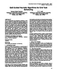
node granularity Gn is less than task granularity GT and condition (4) is not executed, then task granularity GT is reduced to meet conditions (4) and (10). B. Algorithm of the Modified Task Scheduler Function 1. Begin; 2. creation of the task queue; 3. if the task queue is empty, then go to step 19; 4. the selection of the next task; 5. create an available node list at the task downloading time; 6. if the node list is empty, then go to step 5; 7. the selection of node ri с min |GT – Gn| and Ti ≤ TZ /* selection of the node that is most appropriate for criteria ET and En */; 8. if 0.5≤ (GT| Gn ) ≤1.5, then go to step 17; 9. if GT < Gn, then go to step 12 /* task granularity smaller than node granularity */; 10. if GT is minimal, then go to step 17 /* further declustering impossible */; 11. decrease of GT, then go to step 8 /* performed by clustering */; 12. if GT maximum, then go to step 17 /* further clustering violates the condition: Ti ≤ TZ */; 13. increase of GT /* performed by clustering */; 14. the calculation of a Ti new value; 15. if Ti ≤ TZ, then go to step 8; 16. decrease of GT /* performed by declustering */; 17. task immersion on node ri; 18. go to step 2; 19. End. V. ANALYSIS OF THE ALGORITHM’S EFFECTIVENESS FOR THE PROCESS OF SCHEDULING TASKS IN A GRID SYSTEM A. Simulation of the Task Scheduling Process The GridSim [36] modeling system, which allows different scheduling policies to be implemented (FCFS, Easy Backfill, Conservative Backfill) is selected as a tool for modeling and analyzing the effectiveness of the proposed algorithm. In the current research, GridSim has been expanded by adding new necessary entities for the simulation of the planning process and execution of workflows in the grid environment. The class diagrams of the implemented modules are shown in Figure 1.



Fig. 1. Class diagram in the modeling system

A modeling system allows for test task immersion in real time. The number of tasks and resources are defined by the user. The result of both scheduling algorithm simulations, with the same input data, are output data, such as average task downtime in the queue, total system boot time, average system node load, average load of communication channels, average scheduler decision time, and system node load chart. The node parameters are the number of CPUs and the performance of the node channel bandwidth of that node. The task is generated with the granularity, the task weight (the amount of calculations), the estimated runtime for a task at its maximum granularity, and the priority. The task queue is created after generation, sorted by priority, in which the task with the highest priority is at the head of the queue. The scheduler works in real time; all measurements are made in milliseconds.

B. Simulation Results of the Base and Modified Scheduling Algorithm The modeling system generated loading charts of grid system nodes and communication channels. Using this simulation program, the loading of system nodes were analyzed at different ratios between the task number and grid system nodes. Figures 2 and 3 show the relative loading of the first 25 nodes and the communication channels as a percentage of their maximum values in the solution of 100 tasks on 50 grid system nodes. A comparison of Figures 2 and 3 illustrates that the loading of the nodes is relatively low with a relatively small difference between the number of tasks and nodes. Furthermore, the modified algorithm provides more balanced and larger loading compared with the baseline algorithm.



Fig. 2. Relative loading of the first 25 nodes and communication channels as a percentage of their maximum values in the solution of 100 tasks on 50 grid system nodes using the base scheduling algorithm

Figures 4 and 5 show the relative loading of the first 25 nodes and communication channels as a percentage of their maximum values in the solution of 5,000 tasks on 100 grid system nodes.

Fig. 5. Relative loading of the first 25 nodes and communication channels as a percentage of their maximum values in the solution of 5,000 tasks on 100 grid system nodes using the modified scheduling algorithm

A comparison of the loading charts (Figures 2–5) with the increase in task queues indicates that the effectiveness of the modified scheduling algorithm is significantly increased due to the higher and more balanced loading of nodes and communication channels. Experiments were performed for a fixed node number but a variable task number. The base and modified algorithms were modeled, and a histogram was constructed based on the average values for the experiments with tasks as one pair of resources.

Fig. 3. Relative loading the first 25 nodes and communication channels as a percentage of their maximum values in the solution of 100 tasks on 50 grid system nodes using the modified scheduling algorithm

Average Queueing Time for the Task

Considering how to apply the base or modified scheduling algorithm will influence the average residence time of the task in queue (Figure 6), the total system loading time (Figure 7), and the average scheduler decision time (Figure 8). 90000.000 80000.000 70000.000 60000.000 50000.000 40000.000 30000.000 20000.000 10000.000 0.000 Number of Tasks for Loading

Fig. 6. Average residence time of a task in the queue based on the task number using the base and modified algorithms with a fixed number of resources of 100

Fig. 4. Relative loading of the first 25 nodes and communication channels as a percentage of their maximum values in the solution of 5,000 tasks on 100 grid system nodes using the base scheduling algorithm



Figures 9–11 show the simulation results of the base and modified schedulers with a fixed task number and different grid system node numbers. Experiments were performed for a fixed task number but a variable node number. We implemented the model using the base and modified algorithms, and the histograms (Figures 9–11) reflect the average values for the experiments with one pair of resources—tasks. As shown in Figure 9, the average task residence time in a queue using the modified algorithm with different amounts of resources is approximately 50% less than when using the base algorithm because the decision time using the modified algorithm is less than that of the base algorithm.

Fig. 7. Total load time of the system with a fixed number of resources of 100

Fig. 9. Dependence of the average task residence time in a queue with a different number of gird system nodes with a fixed number of tasks of 10,000 Fig. 8. Average decision-making time by the scheduler with a fixed number or resources of 100

As shown in Figure 6, regardless of the task number, the residence time in the queue is less than that in the modified algorithm by an average of 20%. As shown in Figure 7, the total system loading time is significantly reduced with the modified algorithm because the modified algorithm selects the optimal ratio between task granularity and system granularity. The average scheduler decision time regarding the choice of the node for the task immersion using the modified algorithm is essentially independent of the task queue size, unlike the base method. This independence occurs because resource searching continues to loop as long as the desired resource is not found. In the base algorithm, resource searching starts from the beginning each time, which often leads the resource to be linearly dependent on the optimal task number search in the queue.

Fig. 10. Total load time of the system with a fixed number of tasks of 10,000



being used, the task waits for the most productive resource regardless of how much time the scheduler spends deciding on the most favorable site node. Consequently, the task is idle, and the system is underutilized. This is not observed when the modified scheduling algorithm is used because the system time is considerably lower than that when using the base algorithm even though the decision time is longer. Table 1 shows the average test results. We generated 10,000 random tasks that were immersed on 1,000 nodes. TABLE I.

RESULTS OF THE ALGORITHMS

Characteristic Waiting time in the queue Total working time Average nodes loading, % Average loading of communication channels, % Decision time, ms Fig. 11. Average decision-making time by the scheduler with a fixed number of resources of 100

C. Analysis of the Modeling Results The histogram shows the average task residence time in a queue for an increasing number of tasks and a fixed amount of resources and a fixed number of tasks and an increasing number of resources in proportion to each task and resource pair. Thus, the task downtime in a queue for the base algorithm is larger than for the proposed modified algorithm. When the modified scheduler does not review all resources when searching, it does not calculate the task execution time for each item in the search to achieve the optimal time. The histogram shows the significant time gap associated with the generation of each experience for a different number of resources with different productivity. This time gap can greatly increase the waiting time of task immersion for the resource with the base algorithm. The histograms show that the system load is reduced when using the modified scheduler because the main load is not in the highest-performing resource and because tasks are evenly distributed across system resources. This reduces the system time and allows many tasks to be executed earlier compared with the base scheduler. The final histogram shows that using the modified scheduling algorithm increases the decision-making time of the scheduler. Let us analyze why this occurs. The base scheduling algorithm is necessary for a full scan and for calculating the computation time of the task on each resource, which is a time-consuming procedure. In the modified algorithm, a request is sent to the resource manager for the sub-list of resources that will be available at the time of data transfer of the current task. This is the first time value in the total time calculation of decision making. Next, the scheduler waits for a response from the resource manager, which holds the necessary calculations to generate a list; the resource manager then sends a list to the scheduler. After that, the scheduler begins to view the issued list of resources to find the optimal resource for the task. When a resource is found, the scheduler calculates the end of the task on the resource, which also takes time. After these steps, if the base algorithm is

Baseline 52848 17 197 200 19

Modified 9506 4 248 600 45

13

11

2,8015

5,2316

VI. CONCLUSION This paper proposes a modified hierarchical method of task scheduling that increases the efficiency of a grid system by selecting the optimal ratio between task granularity and grid system node granularity on a node on which a given task is immersed. This is accomplished by changing the task granularity via conversion. This ensures a uniform, more balanced load of processors and communication channels between grid system nodes and reduces the residence time of the task in the input task queue. The result is increased productivity in the grid system by an average of 20%. A further performance increase is related to the possibility of changing the granularity of grid system nodes by changing their structure considering the number of physical communication channels in the processors of a particular computing node and through support for a duplex mode of information transmission in communication channels. ACKNOWLEDGMENT This research is supported by King Saud University; Author would express his appreciation to the Deanship of Scientific Research at King Saud University for the provision of funding. [1]

[2]

[3]

[4]

[5] [6]

REFERENCES F. Dong, and G. Selim, ―Scheduling Algorithms for Grid Computing: State of the Art and Open Problems (Technical Report),‖ School of Computing, Queen’s University, Kingston Ontario Rep. 2006–504, 2006. D. Cokuslu, A. Hameurlain, and K. Erciyes, ―Grid resource discovery based on centralized and hierarchical architectures,‖ Int. J. Infonomics, vol. 3, Jan. 2010. T. Ma, S. Shi, H. Cao, W. Tian, and J. Wang, ―Review on Grid Resource Discovery: Models and Strategies,‖ IETE Technical Review, Vol. 29, pp. 213-22, 2012. Mohammed Bakri Bashir, Muhammad Shafie Abd Latiff, Aboamama Atahar Ahmed, Adil Yousif & Manhal Elfadil Eltayeeb, ―Content-based Information Retrieval Techniques Based on Grid Computing: A Review‖, IETE Technical Review, Vol. 30, pp.223- 232, 2013 H. El-Rewini, T. Lewis, and H. Ali, Task scheduling in parallel and distributed systems. Englewood Cliffs, NJ: Prentice Hall, 1994. M. L. Pinedo, Scheduling: Theory, Algorithms, and Systems, 5th ed. New York: Springer Verlag, 2008.


(IJACSA) International Journal of Advanced Computer Science and Applications, Vol. 8, No. 3, 2017 [7]

[8]

[9]

[10]

[11]

[12]

[13]

[14]

[15]

[16] [17]

[18]

[19]

[20]

[21]

F. Xhafa, and A. Abraham, ―Computational models and heuristic methods for Grid scheduling problems,‖ Future Generation Computer Systems, vol. 26, pp. 608–621, Apr. 2010. Y. Zomaya, C. Ward, and B. Macey, ―Genetic scheduling for parallel processor systems: comparative studies and performance issues,‖ IEEE Trans. Parallel Distrib. Syst., vol. 10, pp. 795–812, Aug. 1999. G. Aggarwal, M. Kamboj, C. Singh, and P. Sharma, ―A novel resource scheduling algorithm for computational Grid,‖ Int. J. Applied Information Systems (IJAIS), vol. 4, pp. 34–7, Sept. 2012. R. P. Prado, S. García-Galán, A. J. Yuste, and J. E. M. Expósito, ―Genetic fuzzy rule-based scheduling system for grid computing in virtual organizations,‖ Soft Comput., vol. 15, pp. 1255–1271, Jul. 2011. M. Shojafar, Z. Pooranian, J. H. Abawajy, and M. R. Meybodi, ―An efficient scheduling method for Grid systems based on a hierarchical stochastic Petri net,‖ J. Comput. Sci. Eng., vol. 7, pp. 44–52, Mar. 2013. Y. Yang, G. Wu, J.Chen, and W. Dai, ―Multi-objective optimization based on ant colony optimization in grid over optical burst switching networks,‖ Expert Syst. Appl., vol. 37, pp. 1769–1775, Mar. 2010. C. S. Rao, and D. B. R. Babu, ―A fuzzy differential evolution algorithm for Job scheduling on computational grids,‖ Int. J. Computer Trends Technol., vol. 13 , pp. 72–77, Jul. 2014. B. Ekşioğlu, S. D. Ekşioğlu, and P. Jain, ―A tabu search algorithm for the flowshop scheduling problem with changing neighborhoods,‖ Comput. Ind. Eng., vol. 54, pp. 1–11. Feb 2008. B. Barzegar, A. M. Rahmani, and K. Zamanifar, ―Advanced reservation and scheduling in Grid computing systems by gravitational emulation Local search algorithm,‖ Am. J. Scientific Research, no. 18, pp. 62–70, 2011. J. A. Torkestani, ―A new distributed Job scheduling algorithm for Grid systems,‖ Cybernetics Systems, vol. 44, pp. 77–93. 2013. E. Betzar, A. Xavier, and V. M. Betzar, ―Survey on heuristics based resource scheduling in Grid computing,‖ Indian J. Computer Science Engineering (IJCSE), vol. 5, pp. 9–14, Mar. 2014. G. Guoning T.-L. Huang, and G. Shuai, ―Genetic simulated annealing algorithm for task scheduling based on cloud computing environment (Published Conference Proceedings),‖ in Int. Conf. on Intelligent Computing and Integrated Systems, 2010, pp. 60–63. Z. Pooranian, A. Harounabadi, M. Shojafar, and J. Mirabedini, ―Hybrid PSO for independent Task scheduling in Grid computing to decrease Makespan (Published Conference Proceedings),‖ in Proc. Int. Conf. on Future Information Technol., Singapore, 2011, pp. 435–9. Z. Pooranian, A. Harounabadi, M. Shojafar, and N. Hedayat, ―New hybrid algorithm for Task scheduling in Grid computing to decrease missed Task‖, World Academy of Science, Engineering and Technology International Journal of Computer, Electrical, Automation, Control and Information Engineering, Vol:5, 2011, pp. 262–268, 2011. S. K. Garg, R. Buyya, and H. J. Siegel, ―Time and cost trade-off management for scheduling parallel applications on utility grids,‖ Future Generation Computer Systems, vol. 26, pp. 1344–55, Oct. 2010.

[22] M. Khan, ―Design and analysis of Security aware scheduling in Grid computing environment‖ Int. J. Comput. Sci. Inf. Technol. Research vol. 1, pp.42–50, Dec. 2013. Available: www.researchpublish.com [23] P. Keerthika, and N. Kasthuri, ―A hybrid scheduling algorithm with load balancing for computational Grid‖ Int. J. Advanced Science and Technol., vol. 58, pp. 13–28, 2013. [24] R. Aron, and I. Chana, ―Grid scheduling heuristic methods: state of the Art,‖ Int. J. Computer Information Systems and Industrial Management Applications, vol. 6, pp. 466–73, 2014. [25] Hirales-Carbajal, A. Tchernykh, R. Yahyapour, J. L. González-García, T. Röblitz, and J. M. Ramírez-Alcaraz, ―Multiple workflow scheduling strategies with user run time estimates on a Grid,‖ J. Grid Comput., vol. 10, pp. 325–346, 2012. [26] Forti, ―DAG Scheduling for grid computing systems,‖ Ph.D. Thesis, Dep. Mathematics and Comp. Sci., Univ. Udine, Italy, 2006. [27] P. Chauhan, and Nitin, ―Decentralized Scheduling Algorithm for DAG Based Tasks on P2P Grid,‖ J. Engineering, vol. 2014, pp. 202843, 2014. Available: http://dx.doi.org/10.1155/2014/202843. [28] F. Pop, C. Dobre, and V. Cristea, ―Genetic algorithm for DAG scheduling in Grid environments (Published Conference Proceedings),‖ in Proc. IEEE 5th Int. Conf. Intelligent Computer Communication and Processing, Cluj-Napoca, 2009, pp. 299–305. [29] R. Garg, and A. K. Singh, ―Adaptive workflow scheduling in grid computing based on dynamic resource availability,‖ Engineering Sci.Technol. Int. J., vol. 18, pp. 256–269, Jun. 2015. Available: http://dx.doi.org/10.1016/j.jestch.2015.01.001. [30] M. A. Palis, ―The granularity metric for fine-Grain real-Time scheduling,‖ IEEE Transactions Comput., vol. 54, pp. 1572–1583, Dec. 2005. [31] D. Konieczny, J. Kwiatkowski, and G. Skrzypczynski, ―Parallel search algorithms for the distributed environments,‖ in Proceedings of the 16th IASTED Int. Conf. Applied Informatics, Garmisch-Partenkirchen, Germany, 1998, pp. 324–327. [32] Gerasoulis and T. Yang, ―A Comparison of Clustering Heuristics for Scheduling Directed Acyclic Graphs on Multiprocessors,‖ J. Parallel Distributed Computing, vol. 16, pp. 276–91, Dec. 1992. [33] Maui Scheduler™ Administrator's Guide version 3.2, Copyright © 1999-2014, Adaptive Computing Enterprises. Available: http://docs.adaptivecomputing.com/maui/. [34] Tivoli Workload Scheduler Documentation, Available: http://www01.ibm.com/software/tivoli/ [35] Moab Workload Manager Documentation, Available: http://www.adaptivecomputing. com/ [36] R. Buyya and M. Murshed, ―Gridsim: a toolkit for the modeling and simulation of distributed resource management and scheduling for grid computing,‖ Сoncurrency and Computation: Practice and Experience, vol. 14, pp. 1175–220, Nov.-Dec. 2002.
