Modular Refinement of Hierarchic Reactive Machines - Stony Brook

Modular Refinement of Hierarchic Reactive Machines1 RAJEEV ALUR Department of Computer and Information Science, University of Pennsylvania and RADU GROSU Department of Computer Science, State University of New York at Stony Brook

Scalable formal analysis of reactive programs demands integration of modular reasoning techniques with existing analysis tools. Modular reasoning principles such as abstraction, compositional refinement, and assume-guarantee reasoning are well understood for architectural hierarchy that describes the communication structure between component processes, and have been shown to be useful. In this paper, we develop the theory of modular reasoning for behavior hierarchy that describes control structure using hierarchic modes. From Statecharts to UML, behavior hierarchy has been an integral component of many software design languages, but only syntactically. We present the hierarchic reactive modules language that retains powerful features such as nested modes, mode reuse, exceptions, group transitions, history, and conjunctive modes, and yet has a semantic notion of mode hierarchy. We present an observational trace semantics for modes that provides the basis for mode refinement. We show the refinement to be compositional with respect to the mode constructors, and develop an assume-guarantee reasoning principle. Categories and Subject Descriptors: D.2.2 [Design Tools and Techniques]: State diagrams; D.2.4 [Software/Program Verification]: Formal methods; D.2.1 [Requirements/Specifications]: Languages, Methodologies; F.3.1 [Specifying and Verifying and Reasoning about Programs]: Mechanical verification, Specification techniques General Terms: Modeling languages, Formal verification Additional Key Words and Phrases: Hierarchical state machines, Compositional semantics, Assumeguarantee reasoning, Refinement

1. INTRODUCTION The complexity and subtlety of programming reactive systems, such as telecommunications and avionics software, demands increased design automation and effective debugging tools. Recent advances in formal verification have led to powerful 1 A preliminary version of this paper appears in the Proceedings of the 27th Annual ACM Symposium on Principles of Programming Languages, pp. 390–402, 2000.

Author’s address: R. Alur, Department of Computer and Information Science, University of Pennsylvania, 200 South 33rd Street, Philadelphia, PA 19104. R. Grosu, Department of Computer Science, State University of New York at Stony Brook, Stony Brook, NY 11794-4400, USA. Permission to make digital/hard copy of all or part of this material without fee for personal or classroom use provided that the copies are not made or distributed for profit or commercial advantage, the ACM copyright/server notice, the title of the publication, and its date appear, and notice is given that copying is by permission of the ACM, Inc. To copy otherwise, to republish, to post on servers, or to redistribute to lists requires prior specific permission and/or a fee. c 1999 ACM 0164-0925/99/0100-0111 $00.75
ACM Transactions on Programming Languages and Systems, Vol. TBD, No. TDB, Month Year, Pages 1–??.

2

·

Rajeev Alur and Radu Grosu

design tools for hardware (see [Clarke and Kurshan 1996] for a survey), and subsequently, have brought a lot of hope of their application to reactive programming. The most successful verification technique has been model checking [Clarke and Emerson 1981]. In model checking, the system is described by a state-machine model, and is analyzed by an algorithm that explores the reachable state-space of the model. The state-of-the-art model checkers (e.g. Spin [Holzmann 1997] and Smv [McMillan 1993]) employ a variety of heuristics for efficient search, but are typically unable to analyze models with more than hundred state variables. Consequently, application of formal verification requires augmenting model checking with modular reasoning that allows decomposition of the analysis problem into smaller subproblems, or abstracting a component into a simpler one. Typically, such simplification is done manually, and requires considerable expertise. Much of today’s research in formal verification aims to develop techniques to automate modular reasoning and abstraction techniques. To be able to exploit the design structure effectively for modular reasoning, the modeling language must support syntactically as well as semantically modular constructs. While modern programming languages offer a rich set of modular constructs (e.g. procedures, objects), the standard model checkers assume the model to be a state-transition graph (or a Kripke structure) with no structure. Our first attempt to enrich the modeling language resulted in the definition of reactive modules [Alur and Henzinger 1999]. In this language, an atomic module is a statemachine whose variables are explicitly partitioned into input, output, and private variables. The operations of parallel composition, instantiation, and variable hiding allow building complex modules from atomic ones. The denotational semantics of each module consists of its input and output variables, together with the set of its traces, which captures the observable interaction of a module with its environment. The notion of refinement between two modules is based on inclusion of traces, and provides the basis for abstraction. The refinement relation is compositional with respect to the module operations. Thus, to show that the composite module P1 P2 refines the module Q1 Q2 , it suffices to establish that P1 refines Q1 and P2 refines Q2 . While the compositional proof rule decomposes the verification task of proving implementation between compound modules into subtasks, it may not always be applicable. In particular, P1 may not implement Q1 for all environments, but only if the environment behaves like P2 , and vice versa. For such cases, we must employ the assume-guarantee proof rule which asserts that in order to prove that P1 P2 implements Q1 Q2 , it suffices to prove (1) P1 Q2 implements Q1 , and (2) Q1 P2 implements Q2 . The language of reactive modules, along with the assume-guarantee refinement checker, is supported by the model checker Mocha [Alur et al. 2001], and the utility of the assume-guarantee reasoning has been demonstrated in analysis of a video-graphics image processor [Henzinger et al. 1998] and the network protocol PPP [Alur and Wang 2001]. While the reactive modules language supports architectural hierarchy, it offers little structure to express the behavior of individual modules. In this paper, we present the language of hierarchic reactive modules that supports both architectural and behavioral hierarchy, along with its compositional semantics and assumeguarantee proof calculus. The notion of behavior hierarchy was popularized by the introduction of Statecharts [Harel 1987], and exists in many related modeling ACM Transactions on Programming Languages and Systems, Vol. TBD, No. TDB, Month Year.

Modular Refinement of Hierarchic Reactive Machines

·

3

formalisms such as Modecharts [Jahanian and Mok 1987] and Rsml [Leveson et al. 1994]. It is a central component of various object-oriented software development methodologies developed in recent years, such as Room [Selic et al. 1994], and the Unified Modeling Language (Uml [Booch et al. 1997]). The central component of the behavioral description in our language is a mode. A mode consists of global variables used to share data with its environment, local variables, well-defined entry and exit points, and submodes that are connected with each other by transitions. The transitions are labeled with guarded commands that access the variables according to the the natural scoping rules. Note that the transitions can connect to a mode only at its entry/exit points, as in Room, but unlike Statecharts. This choice is important in viewing the mode as a black box whose internal structure is not visible from outside. The mode has a default exit point, and transitions leaving the default exit are applicable at all control points within the mode and its submodes. The default exit retains the history, and the state upon exit is automatically restored by transitions entering the default entry point. Thus, a transition from default exit to entry models a group transition applicable to all control points inside. While defining the operational semantics of modes, we follow the standard paradigm in which transitions are executed repeatedly as long as at least one is enabled (has a true guard). Since the control can be simultaneously in multiple nested modes, the order in which the transitions are tried for execution is important. Unlike Statecharts, but as in Room, the operational semantics tries the transitions inside out, that is, we give priority to the internal transitions over the group transitions of the enclosing mode. This choice is also crucial for the clean denotational semantics. Our language allows mode instantiation and thus, reuse. Our denotational semantics of a mode consists of its global variables, entry/exit points, and traces over global variables that capture a mode’s behavior. The key step leading to such semantics involves a closure construction that adds transitions connecting the default points. This construction makes the transfer of control between a mode and its environment explicit. Consequently, the behavior of a mode can be viewed as a game in which the environment transfers control to the mode at one of its entry points, and the mode transfers the control back to the environment at one of its exit points. The macro-transition from an entry point to an exit point, thus, consists of multiple transitions, and can be constructed from the macro-transitions of the submodes together with the transition relation of the mode. The macro-transitions are then used to associate a set of executions and a corresponding set of traces with a mode. We show that the traces of a mode can be constructed from the traces of its submodes. The denotational trace semantics naturally leads to a notion of refinement among modes based on inclusion of traces, and provides the basis for mode abstraction and substitution. We show that the constructors are compositional with respect to this refinement relation, and this leads to compositional proof rules for refinement. In particular, to establish that a mode M with a submode N refines a mode M
with submode N
, it suffices to prove that (1) mode N refines N
, and (2) mode M with N substituted by a “free” mode that allows most general update, refines mode M
with N
made free. Thus, compositional rule allows us to decouple the reasoning about a submode from the reasoning about its context. We also present a circular assume-guarantee proof rule in which the specification context M
can be assumed ACM Transactions on Programming Languages and Systems, Vol. TBD, No. TDB, Month Year.

4

·

Rajeev Alur and Radu Grosu

while establishing the first sub-goal, and the specification submode N
can be used while establishing the second sub-goal. Hierarchic languages such as Statecharts allow the notion of conjunctive (parallel) states. We argue that conjunction can be defined cleanly as a constructor over submodes such that a step of the constructed mode consists of a sequence of micro steps, one micro step for each submode. We establish that such a conjunctive constructor is compositional with respect to refinement and that its trace semantics is essentially the same as the trace semantics of the parallel composition constructor over modules. This suggests a scheme for mixing modes and modules interchangeably in system descriptions. Related work This paper develops compositional semantics for hierarchical reactive systems. As discussed earlier, it builds upon the compositional language of reactive modules [Alur and Henzinger 1999]. The notion of compositional refinement based on observable behaviors is central to many other formal models such as CCS [Milner 1980], I/O automata [Lynch and Tuttle 1987], TLA [Lamport 1994]. Languages such as reactive modules, I/O automata and TLA are concerned only with concurrent composition, and thus, only with the architectural hierarchy. In behavior hierarchy, modes at the same level are composed sequentially, and modes at different levels can be active concurrently. Consequently, a language with behavior hierarchy cannot be given a natural and compositional semantics in models that support only concurrent composition. Process algebras such as CCS allow both sequential and concurrent composition, and thus, both architectural and behavioral hierarchies. Compared to process algebras, our formalism differs in the following ways. First, it allows explicit modeling of hierarchy and group transitions that is similar to many visual software design languages. Second, while communication in process algebras uses events (or actions), we use shared variables. Third, the notion of equivalence for process algebras such as CCS is based on bisimulation, while our semantics uses the weaker notion of traces. Another focus of our compositionality is assume-guarantee reasoning. Since assume-guarantee reasoning allows modeling of assumptions about the interface of a component, it promises to be more relevant in decomposing proofs. Due to the inherent circularity, assume-guarantee reasoning [Stark 1985; Abadi and Lamport 1995; Alur and Henzinger 1999; McMillan 1997] is valid only when the interaction of a module with its environment is non-blocking, and is not valid for frameworks such as CCS. The concept of behavioral hierarchy in state-machine-based formalisms can be traced to Statecharts [Harel 1987]. Such hierarchic specifications have many powerful primitives such as exceptions, group transitions, and history, which lead to complex semantics [Harel et al. 1987; Pnueli and Shalev 1991; Harel and Naamad 1996; Huber et al. 1996; Grosu et al. 1998; L¨ uttgen et al. 2000]. There have been several attempts to define a rigorous semantics of Statecharts alone. Typically the semantics is defined operationally by considering the global state of the system. In fact, multiple papers offer a compositional semantics that is congruent with the language constructs [Uselton and Smolka 1994]. However, the notion of semantic equivalence used in all these papers is structural isomorphism of underlying stateACM Transactions on Programming Languages and Systems, Vol. TBD, No. TDB, Month Year.

Modular Refinement of Hierarchic Reactive Machines

·

5

transition graphs (or bisimilarity but with most of the structure visible), rather than conventional observational equivalences. Also there have been attempts to exploit the hierarchic states for efficient reachability analysis [Chan et al. 1998; Alur and Yannakakis 1998; Behrmann et al. 1999]. However, there is no observational semantics that allows defining a refinement preorder on hierarchic states. Thus, the main contribution of this paper is a modular semantics for hierarchical specifications with a supporting trace-based refinement calculus. We hope that it will provide insights for incorporating hierarchical constructs in modeling languages so that the hierarchy is semantic, and will also provide a basis for restricting or adapting popular languages such as Statecharts so that modularity principles such as assume-guarantee reasoning can be applied to their formal analyses. Outline The rest of the paper is organized as follows. In Section 2 we review reactive modules: their syntax, semantics and refinement rules. In Section 3 we follow a similar pattern for modes. We first introduce their syntax and then we define their semantics and refinement rules. Section 4 is devoted to conjunctive modes. First we define conjunction as a particular mode constructor. Then we show that conjunction is compositional with respect to refinement and relate it to module composition. Finally in Section 5 we draw some conclusions. During the entire paper, we use the specification of a small village telephone system, inspired from [Bhargavan et al. 1998], as a working example to illustrate definitions. Notation Given a set V of typed variables, a state over V is a function mapping variables to their values. The set of states over V is denoted QV . Given a state s over V and a subset W of V , s.W denotes the state over W obtained by restricting s to the variables in W . The projection operator extends to sequences of states also. Given two sets V and W of variables, an action from V to W is a binary relation between the states over V and the states over W . An action α from V to W is said to be enabled at a state s over V if (s, t) ∈ α for some state t. An action α from V to W is said to be non-blocking if it is enabled at every state over V . The domain and range of an action can be expanded implicitly in a natural way: if α is an action from V to W , s is a state over V
⊇ V and t is a state over W
⊇ W , then define (s, t) ∈ α if (s.V, t.W ) ∈ α and t.v = s.v for v ∈ (V
∩ W
) \ W . This implicit coercion is quite common and allows one to assume that the variables not explicitly occurring in a transition remain unchanged. 2. MODULES 2.1 Syntax A module is defined by the set of its variables, rules for initializing the variables, and rules for updating the variables. The variables of a module P are partitioned into three classes: private variables that cannot be read or written by other modules, interface variables that are written only by P , but can be read by other modules, and external variables that can only be read by P , and are written by other modules. Thus, interface and external ACM Transactions on Programming Languages and Systems, Vol. TBD, No. TDB, Month Year.

6

·

Rajeev Alur and Radu Grosu c4 c1

h1 h4

..

..

UserSpec h1

...

.. h4

...

Conn1

.. ..

..

Conn4

SelPartn

..

SystemSpec c1

..

p

..

c4

SystemSpec

..

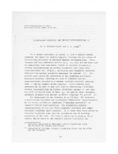
Fig. 1. Architecture diagrams for the VTS variables are used for communication, and are called observable variables. The private and interface variables are written by the module, and are called controlled variables. The execution of a module proceeds in a sequence of rounds. The initialization specifies initial controlled states. The subsequent rounds are update rounds determined by the transition relation which specifies how to change the controlled state as a function of the current state. In each round, the external variables are assigned arbitrary values. Definition 1. (Modules) A module P consists of Variables. A finite set V of typed variables that is partitioned into private variables Vp , interface variables Vi and external variables Ve . The variables in Vc = Vp ∪ Vi are called controlled variables, and the variables in Vo = Vi ∪ Ve are called observable variables. Initial states. A non-empty subset I of states over Vc . ✷ Update relation. A non-blocking action U from V to Vc . Example 1. (Village telephone system) Consider a simple village telephone system that is able to establish a point-to-point connection between any two telephone lines that are disconnected and off hook. For simplicity, assume that the system has only four lines. The block (architecture) diagram for the system and and the users is shown in Figure 1, left. To define and analyze the behavior of the village telephone system, we associate each block in the diagram to a reactive module with the interface shown in the diagram. A high level definition of the environment is the UserSpec module given below. type hookType is {on, off} module UserSpec is interface h1, h2, h3, h4 : hookType; init [] true -> h1 := on; h2 := on; h3 := on; h4 := on; update [] h1 = on -> h1 := off; [] h1 = off -> h1 := on; [] h2 = on -> h2 := off; ACM Transactions on Programming Languages and Systems, Vol. TBD, No. TDB, Month Year.

Modular Refinement of Hierarchic Reactive Machines

[] [] [] [] [] []

h2 = h3 = h3 = h4 = h4 = true

·

7

off -> h2 := on; on -> h3 := off; off -> h3 := on; on -> h4 := off; off -> h4 := on; -> ;

The module has four variables, all of which are interface variables. In this example, the initialization and the update relation is presented using guarded commands. In each update round it may toggle one of the four lines between on and off. The choice is nondeterministic. Due to the last clause, it is also allowed to idle in a round, and thus, to arbitrarily delay toggling. ✷ As the above example shows, reactive modules offer little support for factoring out common (sequential) behavior. The introduction of modes in Section 3 allows more structuring. 2.2 Semantics For a module P , we use the notation P.Vp to refer to the private variables of P , P.U to refer to the update action of P , etc. The semantics of a module is captured by defining its executions and traces: Definition 2. (Traces) An execution of a module P is a sequence s0 s1 · · · sn of states over P.V such that s0 .(P.Vc ) ∈ P.I and (si , si+1 .(P.Vc )) ∈ P.U for 0 ≤ i < n. If σ is an execution of P , then the corresponding sequence σ.Vo of observable states is called a trace of P . The set of all traces of P is called the trace-language of P , ✷ and is denoted LP . The denotational semantics of the module P is captured by its interface variables, external variables, and trace language. The requirement that I is non-empty and U is non-blocking ensures that the module can always take a step, and the trace-set LP is infinite. Remark 1. (Awaits dependencies and sub-rounds) In our definition, the initial values of the controlled variables cannot depend on each other and in each update step, the new values of the controlled variables cannot depend on the new values of the external and controlled variables. Thus, modules are like Moore machines. The definition of reactive modules [Alur and Henzinger 1999] allows specification of a partial order — called awaits dependencies, over variables such that if a variable x is greater than a variable y in this ordering, then the initial value of x can refer to the initial value of y and the update rule for x can refer to the updated value of y. This allows more complex forms of interaction between a module and its environment by splitting each update round into a fixed number of sub-rounds. In this paper, we want to focus on the hierarchical specification of the update relation, so we have chosen a simpler form of interaction with no awaits dependencies for the sake of clarity of presentation. ✷ Remark 2. (Fairness) By labeling subsets of the update relation as strongly or weakly fair one obtains fair modules [Alur and Henzinger 1999]. Fairness is however not the main focus of this paper and it is therefore not further pursued. ✷ ACM Transactions on Programming Languages and Systems, Vol. TBD, No. TDB, Month Year.

8

·

Rajeev Alur and Radu Grosu

2.3 Hierarchy Operators on modules include instantiation, hiding of interface variables, and parallel composition. We first discuss the parallel composition operator that allows to combine two modules into a single one. Definition 3. (Parallel Composition) The modules P and Q are composable if P.Vc ∩ Q.Vc is empty. The composition R of composable modules P and Q, denoted P Q, is the module with: Variables. The sets of interface, external and private variables: R.Vi = P.Vi ∪ Q.Vi ,

R.Ve = (P.Ve ∪ Q.Ve ) \ R.Vi ,

R.Vp = P.Vp ∪ Q.Vp

Initial states. The set R.I = P.I × Q.I. Update relation. The relation R.U such that: (s, t) ∈ R.U

iff

(s.(P.V ), t.(P.Vc )) ∈ P.U ∧ (s.(Q.V ), t.(Q.Vc )) ∈ Q.U

✷

Note that the denotational semantics of P Q can be completely constructed from the denotational semantics of P and Q. This is because a sequence σ belongs to the trace language LP Q iff its corresponding projections belong to the trace languages LP and LQ [Alur and Henzinger 1999]. The hiding operation makes an interface variable a private one, and thus, allows us to construct module abstractions of varying degrees of detail. Definition 4. (Hiding) Given a module P and an interface variable x ∈ P.Vi , the module hide x in P has the set P.Vp ∪ {x} of private variables, the set P.Vi \ {x} of interface variables, the set P.Ve of external variables, the set P.I of initial states, and the action P.U as the update relation. ✷ Starting with atomic modules, the operations of parallel composition and hiding allow us to describe complex modules in a hierarchical way. Example 2. (Village telephone system) A possible hierarchic decomposition of the module SystemSpec is obtained by introducing for each telephone line i a connection module Conni. An additional module SelPartn is used to guide the selection of the communication partner. This defines the architecture shown by the block diagram in Figure 1, right. The blocks marked with a thick arrow represent registers. They separate the current state from the next state. The specification of the module SelPartn is trivial. It nondeterministically chooses one of the selection modes. type matchingType is {"1-2/3-4","1-3/2-4","1-4/2-3"} module SelPartn is interface p : matchingType; init update true -> p := nondet; The specification of the connection module Conn1 is as follows. If the module is disconnected and its line is off hook, then it chooses a partner connection module as specified by the value of p, provided this partner module is also disconnected and its line is off hook. In this case it becomes connected. If the current communication ACM Transactions on Programming Languages and Systems, Vol. TBD, No. TDB, Month Year.

Modular Refinement of Hierarchic Reactive Machines

·

9

partner goes on hook then the module goes in the drooping state. Finally, if its own line goes on hook, then it becomes disconnected. type connectionType is {disconnected, 1, 2, 3, 4, drooping} module Conn1 is interface c1 : connType; external c2,c3,c4 : connType; h1,h2,h3,h4 : hookType; p : matchingType; init [] true -> c1 := disconnected; update [] h1 = on -> c1 := disconnected; [] c1 = 2 & h2 = on -> c1 := drooping; [] c1 = 3 & h3 = on -> c1 := drooping; [] c1 = 4 & h4 = on -> c1 := drooping; [] c1 = disconnected & p = "1-2/3-4" -> c1 [] c1 = disconnected & p = "1-3/2-4" -> c1 [] c1 = disconnected & p = "1-4/2-3" -> c1

h1 := h1 := h1 :=

= off & c2 = disconnected & h2 = off & 2; = off & c3 = disconnected & h3 = off & 3; = off & c4 = disconnected & h4 = off & 4;

The other connection modules are specified in a similar way. Composing the above modules gives the specification of the entire system, as shown below. module SystemSpec is hide p in ( Conn1 .. Conn4  SelPartn ) module Spec is UserSpec  SystemSpec

✷

2.4 Refinement The notion of refinement between successive levels of abstraction is formalized by the definition of the implementation preorder: Definition 5. (Implementation) A module P implements a module Q, written P Q, if P and Q have identical interface variables, identical external variables, ✷ and LP ⊆ LQ . Intuitively, P Q holds if every observable behavior of P is also a possible behavior of Q, and thus, if the implementation P is more constrained than the specification Q. We have required both the modules to have identical observable variables, but this can be generalized in a straightforward way to allow the implementation to have more interface and external variables such that the external variables of the specification are a subset of the external and interface variables of the implementation. Hence, the implementation is allowed to constrain some of the external variables of the specification. A key property of the implementation relation is compositionality which ensures that the refinement preorder is congruent with respect to the module operations [Alur and Henzinger 1999]. ACM Transactions on Programming Languages and Systems, Vol. TBD, No. TDB, Month Year.

10

·

Rajeev Alur and Radu Grosu

Proposition 1. (Compositionality) If P Q then P R QR. By applying the compositionality rule twice and using the transitivity of refinement it follows that, in order to prove that a complex compound module P1 P2 (with a large state space) implements a simpler compound module Q1 Q2 (with a small state space), it suffices to prove (1) P1 implements Q1 and (2) P2 implements Q2 . We call this the compositional proof rule for reactive modules. It is valid, because parallel composition and implementation behave like language intersection and language containment, respectively. While the compositional proof rule decomposes the verification task of proving implementation between compound modules into subtasks, it may not always be applicable. In particular, P1 may not implement Q1 for all environments, but only if the environment behaves like P2 , and vice versa. For such cases, an assumeguarantee proof rule is needed [Stark 1985; Gr¨ umberg and Long 1994; Abadi and Lamport 1995; Alur and Henzinger 1999]. The assume-guarantee proof rule for reactive modules asserts that in order to prove that P1 P2 implements Q1 Q2 , it suffices to prove (1) P1 Q2 implements Q1 , and (2) Q1 P2 implements Q2 [Alur and Henzinger 1999]. Both proof obligations (1) and (2) typically involve smaller state spaces than the original proof obligation, because the complex compound module P1 P2 usually has the largest state space involved. The assume-guarantee proof rule is circular; unlike the compositional proof rule, it does not simply follow from the fact that parallel composition and implementation behave like language intersection and language containment. Rather the proof of the validity of the assume-guarantee proof rule proceeds by induction on the length of traces. For this, it is crucial that every trace of a module can be extended. Proposition 2. (Assume-Guarantee) If P1 Q2 Q1 Q2 and Q1 P2 Q1 Q2 , then P1 P2 Q1 Q2 . The language of reactive modules, along with the assume-guarantee refinement checker, is supported by the model checker Mocha [Alur et al. 2001], and the utility of the assume-guarantee reasoning has been demonstrated in analysis of a video-graphics image processor [Henzinger et al. 1998] and the network protocol PPP [Alur and Wang 2001]. 3. MODES The architectural hierarchy of a system can be formally captured by modules. In this section, we introduce modes to describe the behavior of atomic modules in a structured and hierarchical manner. 3.1 Syntax 3.1.1 Hierarchy. A mode has a refined control structure given by a hierarchical state machine. It basically consists of a set of submode instances SM connected by transitions T such that at each moment of time only one of the submode instances is active. A subset Im ⊆ SM designates the initial submode instances (visually marked with an arrowhead). A submode instance has an associated mode definition. Different instances can be associated with the same definition, but we require that ACM Transactions on Programming Languages and Systems, Vol. TBD, No. TDB, Month Year.

·

Modular Refinement of Hierarchic Reactive Machines

M

e3

read x, write y, local z e2 e1

e1

a

m:N

e2

x2

b

k

x1

x2

j

c

e2 e1

x1

f

d

c

N

e2

read-write z, local u

11

n:N

x1

e

p

e1

x2

i

h

a

f

g

x3

b

q

x1

r

e

d x2

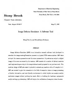
Fig. 2. Scoping rules and transition types the modes form an acyclic graph with respect to this association2. For example, the mode M in Figure 2 contains two submode instances, m and n pointing to the mode N; m is the initial submode instance. By distinguishing between modes and instances we may control the degree of sharing of submodes. For example, the submode instances m and n in Figure 2 share the same mode N. Note that a mode resembles an or state in Statecharts. 3.1.2 Variables. A mode may have global as well as local variables. The set of global variables Vg is used to share data with the mode’s environment. The variables in Vg are classified into a set Vr of read variables and a set Vw of write variables. Hence, Vg = Vr ∪ Vw . The set of local variables Vl of a mode is accessible only by its transitions and submodes. The variables in Vc = Vw ∪ Vl are called controlled variables. Each mode has associated a set of initial states Is over Vc (each controlled variable has to be initialized when first declared). The scoping rules for variables are as in standard structured programming languages. For example, the mode M in Figure 2 has the global read variable x, the global write variable y and the local read-write variable z. Similarly, the mode N has the global read-write variable z and the local read-write variable u. The transitions of a mode may refer only to the declared global and local variables of that mode and only according to the declared read/write permission. For example, the transitions a,b,c,d,e,f,g,h,i,j and k of the mode M may refer only to the variables x, y and z. Moreover, they may read only x and z and write y and z. The global and local variables of a mode may be shared between submode instances if the associated submodes declare them as global (the set of global variables of a submode has to be included in the set of global and local variables of its parent mode). For example, the value of the variable z in Figure 2 is shared between the submode instances m and n. However, the value of the local variable u is not shared between m and n. 3.1.3 Entry/exit points. To obtain a modular language, we require the modes to have well defined control points classified into entry points (marked as white bullets) and exit points (marked as black bullets). For example, the mode M in Figure 2 has the entry points e1,e2, e3 and the exit points x1,x2,x3. Similarly, the mode N has the entry points e1,e2 and the exit points x1,x2. 2 Removing

this restriction one obtains recursive state machines.

ACM Transactions on Programming Languages and Systems, Vol. TBD, No. TDB, Month Year.

12

·

Rajeev Alur and Radu Grosu

The transitions connect the control points of a mode and of its submode instances to each other. For example, in Figure 2 the transition a connects the entry point e2 of the mode M with the entry point m.e1 of the submode instance m. According to the points they connect, the transitions of a mode may be classified into entry, internal and exit transitions. For example, in Figure 2, a,d are entry transitions, h,i,k are exit transitions, b is an entry/exit transition and c,e,f,g,j are internal transitions. Exit transitions implicitly reinitialize (forget) the value of the local variables. 3.1.4 Preemption. To model preemption each mode (instance) has a special, default exit point dx, represented visually as the border of the mode. A transition starting at dx is called a preempting or group transition of the corresponding mode. It may be taken whenever the control is inside the mode and no internal transition is enabled. For example, in Figure 2 left, the transition f is a group transition for the submode n. To achieve the preempting behavior we add for each internal exit point a default exit transition (from this point to dx) that is enabled when all other transitions starting in this point are disabled. These transitions are not explicitly drawn. They are implicit in the semantics of a mode. For example, if the current control point is q inside the submode instance n and neither the transition b nor the transition f is enabled, then the control is transferred to the default exit point dx. If one of e or f is enabled and taken then it acts as a preemption for n. Thus, the inner transitions have a higher priority than the group transitions, that is, we use weak preemption (like the weak kill in Unix, versus the strong kill -9). This priority scheme facilitates a modular semantics. 3.1.5 History. To allow history retention, we use a special default entry point de, represented visually also as the border of the mode. A transition entering the default entry point of a mode restores the values of all local variables along with the position of the control (if the mode was most recently left along one of its explicit exit points then all local variables are reinitialized and control is passed to one of the initial submodes). For example, both transitions e and g in Figure 2, enter the default entry point de of n. The transition e is called a self group transition. A self group transition like e or more generally a self loop like f,p,g may be understood as an interrupt handling routine. While a self loop may be arbitrarily complex, a self transition may do simple things like counting the number of occurrences of an event. To achieve the above behavior we semantically add default entry transitions from the default entry point de of a mode m to its internal points. The default exit transitions save the current point in a local history variable m.h and the default entry transitions restore the current control point from this variable. The initial value of m.h is the default entry point of an initial submode. A mode enriched with default entry and exit transitions is said to be closed . Remark 3. (History free modes) The closure construction is not necessary for modes that have at least one transition enabled at each control point, including de. We call these modes history free. Their set of initial submodes has to be empty. ✷ ACM Transactions on Programming Languages and Systems, Vol. TBD, No. TDB, Month Year.

Modular Refinement of Hierarchic Reactive Machines

·

13

read-write h1,...,h4

read-write h on2off

toggle1 ...

off2on

toggle4

toggle

Fig. 3.

UserSpec

UserSpec for VTS

Remark 4. (Mode instantiation) A mode can be viewed as an encapsulation operator over its submodes. Thus, modes are constructed from leaf-modes using encapsulation repeatedly in a non-recursive manner. Mode instantiation allows reuse and sharing by permitting both to refer to the same mode and to rename a (subset of) entry points, exit points, read variables, and write variables. With mode instantiation, the mode structure is a directed acyclic graph and it can be exploited in an efficient way for model checking [Alur and Yannakakis 1998; Alur et al. 2000]. To simplify the formal definitions in the following we assume a tree like structure obtained by replacing each instance by its corresponding mode. Moreover, we assume that there are no name conflicts regarding local variables and entry/exit points across modes. ✷ Now we are ready to present a formal definition of modes. Definition 6. (Mode) A mode consists of Control points. A finite set E of entry points, and a finite set X of exit points. We also assume an additional default entry point de, and a default exit point dx, and define dE = E ∪ {de}, and dX = X ∪ {dx}. Variables. A finite set Vr of read variables, a finite set Vw of write variables, and a finite set Vl of local variables. The variables Vg = Vr ∪ Vw and Vc = Vw ∪ Vl are called global and controlled variables, respectively. We assume that the sets Vg and Vl are disjoint (but the sets Vr and Vw need not be). Submodes. A finite set SM of submodes. If N is a submode in SM , then it is required that N.Vr ⊆ Vr ∪ Vl and N.Vw ⊆ Vw ∪ Vl . Transitions. A finite set T of transitions of the form (e, α, x), where e is in dE ∪ SM.dX, x is in dX ∪ SM.dE, and α is an action from Vr ∪ Vl to Vw if x ∈ X and from Vr ∪ Vl to Vw ∪ Vl otherwise. We require that for each e ∈ E, the union ∪α such that (e, α, x) ∈ T for some x, is a non-blocking action. Initial states. A non-empty subset Is of states over Vc . Initial submodes. A possibly empty subset Im ⊆ SM of initial submodes. If Im is empty, we require that for each e ∈ {de}∪SM.dX, the union ∪α such that (e, α, x) ∈ T for some x, is a non-blocking action (the mode is history free). Collectively we refer to Is and Im by I. ✷ The interface of a mode is the tuple (Vr , Vw , E, X). A leaf mode is a mode with no submodes and no local variables. A most general mode G(Vr , Vw , E, X) is a mode that has the interface (Vr , Vw , E, X) and imposes no restriction on the update relation (it acts similarly to the environment). ACM Transactions on Programming Languages and Systems, Vol. TBD, No. TDB, Month Year.

·

14

Rajeev Alur and Radu Grosu

read-write c1 read c2, c3, c4 read h1, h2, h3, h4 read p

on disconnected

off2 off3 off4

connected

off2

2

off3

3

off4

4

write c1 read h2, h3, h4

ron2 ron3

drooping

ron4

Conn1

connected

Fig. 4. The mode Conn1 Example 3. (Village telephone system) By using modes, the specification of the module UserSpec may be given by the history free modes UserSpec and toggle as shown in Figure 3. The modes toggle1 to toggle4 are obtained from mode toggle by renaming variable h with h1 to h4 respectively. The unmarked transition connecting de to dx is the identity transition expressing idling. The initial state and the other transitions are defined as follows. read-write h1,h2,h3,h4: def

=

on2off

def

=

off2on

hookType := on

h = on -> h := off h = off -> h := on

The connection module Conn1 may be restated as a hierarchic mode as shown in Figure 4 where initially c1 = disconnected. The transitions are defined as follows. on

def

off2 off3 off4 ron2 ron3 ron4

=

h1 = on -> c1 := disconnected def

=

def

=

def

=

def

=

def

=

def

=

h1 = off & h2 = off & c2 = disconnected & p = "1-2/3-4" -> c1 := 2 h1 = off & h3 = off & c3 = disconnected & p = "1-3/2-4" -> c1 := 3 h1 = off & h4 = off & c4 = disconnected & p = "1-4/2-3" -> c1 := 4 h2 = on -> c1 := drooping h3 = on -> c1 := drooping h4 = on -> c1 := drooping

✷

Note that by distinguishing between control and data, mode diagrams are often more comprehensible than module specifications given by guarded commands. This may have an important impact if the control structure is quite involved and this is the reason why hierarchic state transition diagrams are so popular in software engineering methods. When defining the behavior of a mode in the next section, we regard a mode as a black box, i.e., its submodes and (micro)transitions are hidden. However, in the compositionality proofs for modes, it is sometimes necessary to observe the behavior of a specific submode. Making explicit which submodes are to be observed motivates the introduction of generic modes. ACM Transactions on Programming Languages and Systems, Vol. TBD, No. TDB, Month Year.

Modular Refinement of Hierarchic Reactive Machines

·

15

Definition 7. (Generic mode) A generic mode (or mode context) M [M1 , . . . , Mk ] consists of a mode M along with a set of visible submodes M1 , . . . , Mk . ✷ The visible submodes can also be viewed as the formal parameters of the generic mode. They can be substituted by other, compatible submodes. To simplify the presentation we consider only one visible submode. However, all results apply to the general case. Definition 8. (Compatible modes) A mode M and a mode N are said to be compatible if M.Vr = N.Vr , M.Vw = N.Vw , M.E = N.E and M.X = N.X. ✷ If M [P ] is a generic mode, and the submode P is compatible with a mode Q then M [Q] is the generic mode obtained by substituting P by Q; M [P ] is the non-generic mode obtained by hiding P . Hence M [P ] = M . However, M = M [Q] because they contain different submodes and M = M [P ] because P is hidden in M and visible in M [P ]. Remark 5. (Choice of the language) Our goal is to show how behavior hierarchy can be handled semantically; a design language to be used by practicing software engineers would require many enhancements (such as parametric modes, rich set of data types and expressions). We had to make many choices to make the definition of hierarchy concrete. We discuss these choices by comparing them with the popular language Statecharts. As in Statecharts, multiple nested modes at different levels of hierarchy can be active simultaneously. Modes at the same level of hierarchy are composed only sequentially (that is, only one mode is active at any point in time). Statecharts, on the other hand, allows both sequential and concurrent composition of modes at the same level, and later we will illustrate how concurrent modes can be modeled in our language. In Statecharts, communication is by instantaneous broadcast of events. Events issued by one mode are available to all modes, and consequently, there can be no truly modular semantics of Statecharts. We have chosen shared-variables based communication, and the standard scoping rules are essential to our modular semantics. Entry and exit points in our language are inspired by the modeling language supported by UML-RT. Semantically, the critical entry/exit points are the default ones. These default points are used in the closure construction, to be discussed in the next section, which allows us to express transfer of control between a mode and its environment in a modular fashion. Transitions starting from default exit points allow modeling of exceptions and group transitions. This powerful feature is present in Statecharts as well as UML-RT, and our modular treatment of this feature is an important contribution. We allow both interleaving and synchronous semantics for top-level modes (that is, modules), and when a mode is chosen, it executes transitions until the control reaches one of its exit points (or no more enabled transitions are available). Alternative choices are possible. However, the choice for assigning higher priority to the inside transitions than the outside group transitions is necessary for modularity. ✷ 3.2 Operational Semantics We introduce some additional notation to formally define the set of executions of a mode. For a (generic) mode M we use O to denote the set dE ∪ dX of observable control points and C to denote the set dE ∪ dX ∪ SM.dE ∪ SM.dX of all control ACM Transactions on Programming Languages and Systems, Vol. TBD, No. TDB, Month Year.

·

16

Rajeev Alur and Radu Grosu

M

e3

d

c e2 e1

e1

a b x1

m:N

f

n:N j

k

i x2

N

h

e

p

e1

a

g

x3

q f x1

b e

c

r

e2

d x2

Fig. 5. Closed behavior diagrams points. Pairs of the form (c, s), where c is a control point and s is a state are called configurations. For notational convenience, we view the set T of transitions also as a binary relation over configurations: if (e, α, x) ∈ T and (s, t) ∈ α, we write ((e, s), (x, t)) ∈ T . 3.2.1 The priority among transitions. In Figure 5, the execution of a mode, say n, starts when the environment transfers the control to one of its entry points e1 or e2. The execution of n terminates either by transferring the control back to the environment along the exit points x1 or x2 or by “getting stuck” in q or r as all transitions starting from these leaf modes are disabled. In this case the control is implicitly transferred to M along the default exit point n.dx. Then, if the transitions e and f are enabled, one of them is nondeterministically chosen and the execution continues with n and respectively with p. If both transitions are disabled the execution of M terminates by passing the control implicitly to its environment at the default exit M.dx. Thus, the transitions within a mode have a higher priority compared to the group transitions of the enclosing modes. 3.2.2 Default exit transitions. In any mode, some transition leaving an entry point is guaranteed to be enabled, so execution can get stuck only at an exit point of a submode. In Figure 5 these points are explicitly drawn as black bullets. To make the transfer of control explicit, we add default exit transitions as follows. From an exit point x of a submode of M , we add a transition to the default exit point dx that is enabled if and only if all the explicit outgoing transitions from x are disabled. If the actions are given by guarded commands, and if g1 , . . . ,gn are the guards of the explicit transitions, the guard of the default transition is ¬(g1 ∨ . . . ∨gn ). For example, in Figure 5, the default exit transitions starting in q and r have the guards ¬(gb ∨ gf ) and ¬(ge ∨ gd ) respectively, where gb , gd , ge , gf are the guards of the transitions b,d,e,f, respectively. Similarly, the default exit transition starting in n.dx has the guard ¬(ge ∨ gf ) and the default exit transition starting in p has the guard ¬gg . Each default exit transition saves the local state which is restored upon the subsequent entry to the default entry point. To remember the location of control, we add a new local variable h to a mode M and an action body to each default exit transition (from an exit point x to dx) that saves x in this history variable h. 3.2.3 Default entry transitions. The transitions entering the default entry point of a mode M restore the local state. Again, we introduce explicit default entry ACM Transactions on Programming Languages and Systems, Vol. TBD, No. TDB, Month Year.

Modular Refinement of Hierarchic Reactive Machines

·

17

transitions to restore the location of control. For each default exit transition from an exit x of a submode of M , there is a default entry transition from de to x that is taken when the value of the local history variable h coincides with x. If x was a default exit point n.dx of a submode n then, as shown in Figure 5, the default entry transition is directed to n.de. The reason is that in this case, the control was blocked somewhere inside of n and default entry transitions originating in n.de will restore this control. The closure of the mode M of Figure 2 is shown in Figure 5, where each gray bidirectional arrow represents two unidirectional arrows. The closure construction is defined formally below. Definition 9. (Closure) Let M = (E, X, Vr , Vw , Vl , SM, T, I) be a mode. The closure c(M ) of M is defined to be: (1) M if SM is empty, (2) (E, X, Vr , Vw , Vl , c(SM ), T, I) if M is history free, and (3) (E, X, Vr , Vw , Vl ∪ {h}, c(SM ), dT, dI) otherwise. c(SM ) is the set of closed submodes where c(SM ) = {c(m) | m ∈ SM }. dI is the set of initial states and modes extending Is with an initial value for h in Im .de. dT is a set of transitions obtained from T by adding reinitialization of local variables to the exit transitions and by adding, for each exit x ∈ SM.dX, the transitions (x, αx , dx) and (de, βx ,˜x), where —for x ∈ SM.X,˜x = x, and for x = N.dx,˜x = N.de, —for states s and t, (s, t) ∈ αx iff t.h = x, t.y = s.y for y = h, and for every transition (x, α, x
) in T , α is disabled at s, —for states s, (s, s) ∈ βx iff s.h = x. ✷ Now we proceed to define the operational semantics. Intuitively, a round of the machine associated to a mode starts when the environment passes the updated state along a mode’s entry point and ends when the state is passed to the environment along a mode’s exit point. All the internal steps (the micro steps) are hidden. We call a round also a macro step. Note that the macro step of a mode is obtained by alternating its closed transitions and the macro steps of the submodes. Definition 10. (Macro transitions of modes) The set Vp of private variables of a mode M = (E, X, Vr , Vw , Vl , SM, T, I) is defined to be the set Vl ∪ SM.Vp . The set mT of macro-transitions consists of transitions of the form (e, α, x) with e ∈ dE, x ∈ dX, and α is the action from from Vr ∪ Vp to Vw ∪ Vp , defined as follows. Given the macro-transitions of the submodes of M , a micro-execution of M is a sequence of the form (e0 , s0 ) → (e1 , s1 ) → · · · → (en , sn ) of control points ei ∈ C and states si over Vg ∪ Vp such that —for even i, the transition ((ei , si ), (ei+1 , si+1 )) is in the closure dT of T , —for odd i, the transition ((ei , si ), (ei+1 , si+1 )) is in SM.mT . Given such an execution for an entry point e0 and an exit point en of M , the macro-transition relation mT contains ((e0 , s0 ), (en , sn )). ✷ In the above definition of micro-executions of a mode, the states si are valuations to the variables Vg ∪ Vp , but only a subset of these influence each step. The other remain unchanged. The operational semantics of a mode M consists of its control points, global variables, private variables, and its macro-transitions. ACM Transactions on Programming Languages and Systems, Vol. TBD, No. TDB, Month Year.

18

· dE N.dX

mT

Rajeev Alur and Radu Grosu

M[N] N.dE

N.mT

mT

N.mT

mT

env

...

mT

N.dE N.dX dX

Fig. 6. The traces of M [N ] Remark 6. (Consistency of modes) To ensure consistency we assume the closed transition relation contains no cycles. In the finite state case, checking for cycles is easy. In the infinite state case, one can check for sufficient conditions. For example, one can check for the occurrence of a predefined “wait” mode within each cycle. This mode contains two explicit points e and x and two identity transitions: one from e to dx and one from de to x. ✷ A top-level mode is a mode M with default entry/exit points only. Such a mode can be viewed as a module with private variables Vp , interface variables Vw , external variables Vr \ Vw , initialization specified by the initial states and update specified by macro-transitions from de to dx. For example, mode Conn1 is a top-level mode. The operational semantics of a mode context M [N ] is defined the same way as that of a mode, except that the submode N and the transfer of control between the mode M and the submode N is visible. Thus, a macro step of M [N ] starts either at an entry point of M or at an exit point of N , and terminates at an exit point of M or at an entry point of N . Definition 11. (Macro transitions of generic modes) For a generic mode M [N ], the macro-transition relation mT contains the pair ((e, s), (e
, s
)) if e ∈ M.dE ∪ N.dX, e
∈ M.dX ∪ N.dE, s and s
are states over M.Vg ∪ M.Vp , and there is a ✷ micro-execution of M from (e, s) to (e
, s
). The operational semantics of a generic mode M [N ], consists of the visible control points M.O ∪ N.O, global variables M.Vg , private variables M.Vp , macro-transition relation of M [N ], and the operational semantics of the submode N . 3.2.4 Trace Semantics. The execution of a mode may be best understood as a game, i.e., as an alternation of moves, between the mode and its environment. In a mode move, the mode gets the state from the environment along its entry points. It then keeps executing until it gives the state back to the environment along one of its exit points. In an environment move, the environment gets the state along one of the mode’s exit points. Then it may update any variable except the mode’s private ones. Finally, it gives the state back to the mode along one of its entry points. An execution of a mode is obtained by repeating the mode and environment moves, and a trace is obtained from an execution by retaining only the global states. Definition 12. (Denotational semantics of modes) An execution of a mode M is a sequence (e0 , s0 ) → (x0 , t0 ) → (e1 , s1 ) → (x1 , t1 ) → · · · → (xn , tn ) ACM Transactions on Programming Languages and Systems, Vol. TBD, No. TDB, Month Year.

Modular Refinement of Hierarchic Reactive Machines

·

19

of control points ei ∈ dE, xi ∈ dX with e0 in E, s0 .Vc in I and states si and ti over Vg ∪ Vp such that for all i, ((ei , si ), (xi , ti )) ∈ mT and si+1 .Vp = ti .Vp . Given such an execution, the corresponding trace of M is obtained by projecting each state to the set Vg of global variables. The set of traces of M is denoted LM . The denotational semantics of a mode M consists of its observable points O, global variables Vg , and the set LM of traces. ✷ Note that, for a top level mode, the environment is another reactive module. For a lower level mode, the environment may be a regular or a group transition. The execution of a generic mode M [N ] can be defined similarly as alternation of moves of three kinds. The context mode M gets the state at an entry point or at an exit point of its submode N . It keeps executing until it gives the state back to the environment along one of its exit points or to the submode N at one of the entry points of N . The environment gets the state along one of the exit points of M . It possibly updates the global variables of M , and returns the state to the context M along one of the entry points of M . The submode N gets the state at one of its entry points. It executes one of its macro transitions, and returns the state to M at one of the exit points of N . To obtain a trace from an execution, we retain, at each control point, the values of the variables global at that point. For a mode context M [N ], for a control point c ∈ M.dX ∪ M.dE, let c.Vg be M.Vg , and for a control point c ∈ N.dX ∪ N.dE, let c.Vg be N.Vg . Definition 13. (Denotational semantics of generic modes) An executions of a generic mode M [N ] is a sequence (e0 , s0 ) → (x0 , t0 ) → (e1 , s1 ) → (x1 , t1 ) → · · · → (xn , tn ) of control points ei ∈ M.dE ∪ N.dX, xi ∈ M.dX ∪ N.dE, and states si and ti over M.Vg ∪ M.Vp such that —the execution starts at e0 ∈ M.dE with s0 .(M.Vc ) ∈ M.I, —for all i, ((ei , si ), (xi , ti )) is a macro-transition of M [N ], —for all i, if xi ∈ N.dE then ei+1 ∈ N.dX, and —for all i, the pair ((xi , ti ), (ei+1 , si+1 )) is in N.mT if xi ∈ N.dE and si+1 .Vp = ti .Vp otherwise. Given such an execution, a trace of M [N ] is obtained by projecting each state associated with a point c to the set c.Vg . The set of traces of M [N ] is denoted as before by LM[N ] . The denotational semantics of a generic mode M [N ] consists of the observable points and global variables of M , the observable points and global ✷ variables of N and the set of traces LM[N ] . In order to show that our trace semantics is compositional, we need to be able to define the semantics of a mode M only in terms of the trace semantics of its submodes. This is the same as being able to compute the set of traces of the generic mode M [N ] in terms of the traces of N . Recall that an execution of a generic mode is obtained by alternating between its macro-transitions, its visible submodes macrotransitions and environment transitions (see Figure 6). To formalize the notion of compositionality, we need to define a projection operation for trace-like sequences. ACM Transactions on Programming Languages and Systems, Vol. TBD, No. TDB, Month Year.

20

·

Rajeev Alur and Radu Grosu

Definition 14. (Trace extraction) Given a sequence σ = (e0 , s0 )(e1 , s1 ) . . . (en , sn ) of control points and states, and a mode N , the restriction σ ⇑ N is the sequence obtained from σ by replacing each si by si .(N.Vg ) and by deleting pairs (ei , si ) if ei ∈ N.dE ∪ N.dX. Similarly, σ↑N is the sequence obtained from σ by replacing each si by si .(N.V ) and by deleting pairs (ei , si ) if ei ∈ N.dE ∪ N.dX. ✷ Recall that G(Vr , Vw , E, X) denotes the most general mode with the given set of read/write variables and control points. For a generic mode M [N ], we will use M [G] to denote the generic mode obtained by replacing N with the most general mode G(N.Vr , N.Vw , N.E, N.X). The next lemma captures the essence of compositionality of trace semantics for the encapsulation. Lemma 1. (Trace construction) Let M [N ] be a generic mode, and let τ be a sequence of the form (c0 , s0 ) → (c1 , t1 ) → (c2 , s2 ) → (c3 , s3 ) → · · · → (cn , sn ) such that each ci is in M.dE ∪ N.dE ∪ M.dX ∪ N.dX, and each si is a state over ci .Vg . Then τ is a trace of M [N ] iff τ is a trace of M [G] and τ ⇑ N is a trace of N . Proof. Consider a sequence τ of the form (c0 , s0 ) → (c1 , t1 ) → (c2 , s2 ) → (c3 , s3 ) → · · · → (cn , sn ) such that each ci is in M.dE ∪ N.dE ∪ M.dX ∪ N.dX, and each si is a state over ci .Vg . Suppose τ is a trace of M [N ], and let α be the corresponding execution. Then α↑N is an execution of N , and hence, τ ⇑ N is a trace of N . From α, if we project out the private variables of N , then, by definition of the most general mode, we get an execution of M [G], and thus, τ is a trace of M [G]. Suppose τ is a trace of M [G] and τ ⇑ N is a trace of N . Let α be an execution of M [G] corresponding to τ and β be an execution of N corresponding to τ ⇑ N . Then α and β must have the form (c0 , u0 ) → (c1 , u1 ) → (c2 , u2 ) → (c3 , u3 ) → · · · → (cn , un ) (ci , vi ) → (ci+1 , vi+1 ) → (cj , vj ) → (cj+1 , vj+1 ) · · · → (cm , vm ) and agree on the global variables, i.e., for each ci in β, ui .(N.Vg ) = vi .(N.Vg ). Construct a new sequence γ from α by replacing ui .(N.Vp ) with vi .(N.Vp ) at points ci in β and repeating the last values vi .(N.Vp ) at the intermediate points. By construction, the N -transitions of γ are in N.mT . Moreover, since the environment cannot observe the private variables of N , the M -transitions of γ are in mT . Hence γ is an execution of M [N ]. As a consequence, τ is a trace of M [N ]. The above lemma is used to prove the following theorem which says that to compute the set of traces of a mode M , only the set of traces of its submode, and not the internal structure of the submode, is needed. Theorem 1. Trace construction For a generic mode M [N ], the set of traces of M can be computed from the set of traces of the submode N and the set of traces of M [G]. Proof. The set of traces of M [N ] is computed as in Lemma 1. Then, the traces in LM are the sequences σ ⇑ M where σ ∈ LM[N ] . ACM Transactions on Programming Languages and Systems, Vol. TBD, No. TDB, Month Year.

·

Modular Refinement of Hierarchic Reactive Machines G N

N

< N’

G

M

N’

< M


skip; h1 = on -> skip; h2 = on -> skip; h2 = off -> c1 := 2; c2 := 1; h1 = off -> c1 := 2; c2 := 1; h1 = on -> c1 := disconnected; c2 := drooping;

ACM Transactions on Programming Languages and Systems, Vol. TBD, No. TDB, Month Year.

28

·

Rajeev Alur and Radu Grosu h1 h2 c2disc h1on?

1 h1off?

0

h2off?

6

h1off?

h1on? conn2

4

Line1

diDr1

3 diDr2

h2on?

2

c1 c2

c2disc

conn1

Line2

5

h2on? c1disc

7

h2off?

c1disc

h3 h4

c3 c4

SystemImp

Line1

Fig. 13. Hot lines implementation diDr2

def

=

def

c2disc =

def

c1disc =

h2 = on -> c2 := disconnected; c1 := drooping; h2 = on -> c2 := disconnected; h1 = on -> c1 := disconnected;

We would like now to prove by assume/guarantee that UserImp  SystemImp UserSpec  SystemSpec. This can be done in a mixed module/modes setting or solely in a modes setting by converting the above modules to modes. In this case, we can use the assume/guarantee rule for modes. Let SystemImpPar be the top level mode for the parallel composition together with the mode for SystemImp and SystemSpecPar be the top level mode for the parallel composition together with the mode for SystemSpec. Then we have to prove that SystemImpPar[UserSpec] SystemSpecPar[UserSpec] SystemSpecPar[UserImp] SystemSpecPar[UserSpec] It is easy to see that in this case the assume/guarantee rule for modes is the same as the one for modules. ✷ 5. CONCLUSIONS The notion of hierarchy is useful for structuring architecture of component connections as well as for describing behavior of individual components. While architectural hierarchy has been well understood in context of modular reasoning, there has been no basis for modular reasoning about behavior hierarchy. Existing languages for hierarchic state-machines have complex operational semantics and no notion of observational refinement. We show that hierarchy can be preserved in observational trace semantics even in presence of powerful features such as mode hierarchy, exceptions, history retention, conjunctive modes, and mode reuse. Our language has powerful rules for refinement of modes, and should provide a basis for systematic development and formal analysis of hierarchic descriptions. The current proposal builds on our previous work on the language of reactive modules, the toolkit Mocha that supports assume-guarantee refinement checks and the relational semantics for hierarchic machines in [Grosu et al. 1998]. The operations of building a mode by connecting submodes, scoping of local variables, and ACM Transactions on Programming Languages and Systems, Vol. TBD, No. TDB, Month Year.

Modular Refinement of Hierarchic Reactive Machines

·

29

mode instantiation, are direct analogs of parallel composition of modules, variable hiding, and module instantiation, respectively. Indeed, the same graphical-userinterface can be used for both the module diagrams and mode diagrams. In [Alur et al. 2000] we report on the GUI and a model checker for hierarchic modes. Acknowledgments We thank Manfred Broy, Carl Gunter, Tom Henzinger, Michael McDougall, Amir Pnueli, Bran Selic, Gheorghe Stefanescu and Mihalis Yannakakis for fruitful discussions and suggestions. We also wish to thank the anonymous reviewers for useful comments. Rajeev Alur was partially supported by DARPA/NASA grant NAG2-1214, NSF CARRER award CCR-9734115, SRC award 99-688, Sloan Faculty Fellowship, DARPA ITO Mobies award F33615-00-C-1707, and Bell Laboratories. Radu Grosu was partially supported by NSF CARRER award CCR-0133583. REFERENCES Abadi, M. and Lamport, L. 1995. Conjoining specifications. ACM TOPLAS 17, 507–534. Alur, R., de Alfaro, L., Grosu, R., Henzinger, T., Kang, M., Majumdar, R., Mang, F., Kirsch, C., and Wang, B. 2001. Mocha: A model checking tool that exploits design structure. In Proceedings of 23rd International Conference on Software Engineering. 835–836. Alur, R., Grosu, R., and McDougall, M. 2000. Efficient reachability analysis of hierarchical reactive machines. In Computer Aided Verification: 12th International Conference. LNCS 1855. Springer, 280–295. Alur, R. and Henzinger, T. 1999. Reactive modules. Formal Methods in System Design 15, 1, 7–48. Invited submission to FLoC’96 special isuue. A preliminary version appears in Proc. 11th LICS, 1996. Alur, R. and Wang, B. 2001. Verifying network protocol implementations by symbolic refinement checking. In Computer Aided Verification: 13th International Conference. LNCS 2102. Springer, 169–181. Alur, R. and Yannakakis, M. 1998. Model checking of hierarchical state machines. In Proceedings of the Sixth ACM Symposium on Foundations of Software Engineering. 175–188. Behrmann, G., Larsen, K., Andersen, H., Hulgaard, H., and Lind-Nielsen, J. 1999. Verification of hierarchical state/event systems using reusability and compositionality. In TACAS ’99: Fifth International Conference on Tools and Algorithms for the Construction and Analysis of Software. LNCS 1579. Springer, 163–177. Bhargavan, K., Gunter, C., Gunter, E., Jackson, M., Obradovic, D., and Zave, P. 1998. The village telephone system: A case study in formal software engineering. In Theorem Proving in Higher Order Logics: 11th International Conference. LNCS 1479. Springer, 49–66. Booch, G., Jacobson, I., and Rumbaugh, J. 1997. Unified Modeling Language User Guide. Addison Wesley. Chan, W., Anderson, R., Beame, P., Burns, S., Modugno, F., Notkin, D., and Reese, J. 1998. Model checking large software specifications. IEEE Transactions on Software Engineering 24, 7, 498–519. Clarke, E. and Emerson, E. 1981. Design and synthesis of synchronization skeletons using branching time temporal logic. In Proc. Workshop on Logic of Programs. LNCS 131. Springer, 52–71. Clarke, E. and Kurshan, R. 1996. Computer-aided verification. IEEE Spectrum 33, 6, 61–67. Grosu, R., Stefanescu, G., and Broy, M. 1998. Visual formalisms revisited. In CSD’98, International Conference on Application of Concurrency to System Design. IEEE, 41–51. ¨ mberg, O. and Long, D. 1994. Model checking and modular verification. ACM Transactions Gru on Programming Languages and Systems 16, 3, 843–871. Harel, D. 1987. Statecharts: A visual formalism for complex systems. Science of Computer Programming 8, 231–274. ACM Transactions on Programming Languages and Systems, Vol. TBD, No. TDB, Month Year.

30

·

Rajeev Alur and Radu Grosu

Harel, D. and Naamad, A. 1996. The statemate semantics of statecharts. ACM Trans. Software Engin. Methods 5, 4, 293–333. Harel, D., Pnueli, A., Schmidt, J., and Sherman, R. 1987. On the formal semantics of statecharts. In Proc. 2nd IEEE Symposium on Logic in Computer Science. 54–64. Henzinger, T., Qadeer, S., and Rajamani, S. 1998. You assume, we guarantee: Methodology and case studies. In CAV 98: Computer-aided Verification. LNCS 1427. Springer, 521–525. Holzmann, G. 1997. The model checker SPIN. IEEE Trans. on Software Engineering 23, 5, 279–295. Huber, F., Schtz, B., Schmidt, A., and Spies, K. 1996. Autofocus - a tool for distributed systems specification. In Proceedings FTRTFT’96 - Formal Techniques in Real-Time and Fault-Tolerant Systems. Springer Verlag, LNCS 1135, 467–470. Jahanian, F. and Mok, A. 1987. A graph-theoretic approach for timing analysis and its implementation. IEEE Transactions on Computers C-36, 8, 961–975. Lamport, L. 1994. The temporal logic of actions. ACM Transactions on Programming Languages and Systems 16, 3, 872–923. Leveson, N., Heimdahl, M., Hildreth, H., and Reese, J. 1994. Requirements specification for process control systems. IEEE Transactions on Software Engineering 20, 9, 684–707. ¨ ttgen, G., van der Beeck, M., and Cleaveland, R. 2000. A compositional approach to Lu Statecharts semantics. In Proceedings of the Eighth International Symposium on Foundations of Software Engineering. 120–129. Lynch, N. and Tuttle, M. 1987. Hierarchical correctness proofs for distributed algorithms. In Proceedings of the Seventh ACM Symposium on Principles of Distributed Computing. 137–151. McMillan, K. 1993. Symbolic model checking: an approach to the state explosion problem. Kluwer Academic Publishers. McMillan, K. 1997. A compositional rule for hardware design refinement. In CAV 97: ComputerAided Verification. LNCS 1254. 24–35. Milner, R. 1980. A Calculus of Communicating Systems. LNCS 92. Springer. Pnueli, A. and Shalev, M. 1991. What is in a step: On the semantics of statecharts. In Proc. Symposium on Theoretical Aspects of Computer Software. LNCS 526. Springer, 244–264. Selic, B., Gullekson, G., and Ward, P. 1994. Real-time object oriented modeling and design. J. Wiley. Stark, E. 1985. A proof technique for rely-guarantee properties. In FST & TCS 85, Foundations of Software Technology and Theoretical Computer Science. LNCS 206. Springer, 369–391. Uselton, A. and Smolka, S. 1994. A compositional semantics for statecharts using labeled transition systems. In CONCUR’94: Concurrency Theory, Fifth International Conference. LNCS 836. Springer, 2–17.

ACM Transactions on Programming Languages and Systems, Vol. TBD, No. TDB, Month Year.