MONTE CARLO SIMULATIONS OF THE WHITE DWARF ... - CiteSeerX

To appear in \White Dwarfs: Proceedings of the 10th European Workshop on White Dwarfs", eds. J. Isern, M. Hernanz and E. Garc a-Berro (Kluwer).

MONTE CARLO SIMULATIONS OF THE WHITE DWARF POPULATION AND LUMINOSITY FUNCTION MATT A. WOOD Department of Physics and Space Sciences Florida Institute of Technology Melbourne, FL 32901-6988

Abstract.

The white dwarf luminosity function has been used in recent years as an independent probe of the age and evolution of the local Galactic disk. A long-standing uncertainty of the technique is that the reality of the reported downturn in the luminosity function hinges on just a handful of stars and on statistical arguments that fainter (older) objects would have been observed were they present. Using a Monte Carlo approach, I explore the uncertainties in the derived ages and star formation rates resulting from the small-number statistics of the lowest-luminosity bin. The results suggest that (i) Schmidt's 1=Vmax technique underestimates by typically 25 to 50% the true space density of white dwarf stars in surveys with proper motion limits 00lim<  1:000 yr?1, and (ii) there is 1 Gyr statistical uncertainty in the age inferred from a sample with N<  5 objects in the lowest-luminosity bin, con rming the conservative error estimates adopted by LDM and OSWH.

1. Introduction The practical application of white dwarf (WD) cosmochronometry begins with Winget et al. (1987) and Liebert, Dahn, & Monet (1988; hereafter LDM). Schmidt (1959) rst suggested that observations of the coolest white dwarfs interpreted through Mestel cooling theory could provide an independent age estimate for the local Galactic disk, and D'Antona & Mazzitelli (1978) rst laid out the method for calculating theoretical luminosity functions (LFs), but it was not until the late 1980's that the observational determination of the downturn in the LF near M  16:5 [log(L=L )  ?4:4] was suciently secure to allow detailed theoretical interpretation. These inV

2

MATT A. WOOD

terpretations followed en masse (see Winget et al. 1987, Yuan 1992, Wood 1992, Hernanz et al. 1994, Wood & Oswalt 1997, and references therein). These eorts gleaned all information available from the LDM data, but one long-standing worry about the observed LF is that there are 3 or less objects in the lowest-luminosity bin, depending upon which binning is used. Recently, Oswalt et al. (1996, OSWH) published an independent determination of the WDLF using WDs in common proper motion binaries. This sample includes fainter objects than found in LDM, suggesting a local age of 9.5 Gyr using the thick DA models of Wood (1995) | some 2 Gyr older than the age obtained using these same models to t the LDM LF. The OSWH sample also suggests a factor of 2 larger space density than the LDM sample. These discrepancies have reopened the question of the absolute reliability of LFs calculated with small (N  50) samples and using the 1=Vmax method of Schmidt (1968). To test the behavior of the 1=Vmax method as applied to the observed WD sample, I wrote a simple Monte Carlo (MC) simulation code. I discuss the code brie y and the results more extensively in the remainder of this paper (see also Wood & Oswalt 1997 for a more detailed discussion).

2. The Simulation Program MCGoLF The code mcgolf (= Monte Carlo Generator of Luminosity Functions)

draws pseudo-random samples from a parent sample which is kinematically similar to the observed sample. The x (j = 1; 2; 3) positions are drawn randomly in the rst octant, and the velocities are drawn from a normal (Gaussian) distribution with center and width of vrms = 40 km s?1 . Once the phase-space coordinates are assigned, mcgolf discriminates based on an integrated LF computed with the code lfint (see Wood 1992), as follows. First, on input the integrated LF is put on a linear scale and normalized to a peak of unity. Then for each trial object, two random numbers are drawn. The rst is scaled to provide a value for the trial luminosity `test  log(L=L )test between 0 and ?8. The spline-interpolated value of the integrated LF at this random trial luminosity, lfint (`test), is compared with the value of the second random number test. If test < lfint(`test), then the object \exists" in the sample volume Vsamp at the location (x ; v ; `) and contributes to the overall space density true = Ntot=Vsamp, where Ntot is the total number of objects existing in Vsamp whether in the \observationallyselected" subsample or not. Having now a procedure for populating a space with objects that have luminosities drawn from a probability distribution function de ned by integrated LFs of various ages, the next step is to determine whether a particular object makes it into the \observationally-selected" sub-sample | j

j

j

MONTE CARLO SIMULATIONS OF THE WDLF

3

i.e., whether the proper motion and V magnitude are within the speci ed observational limits. Objects are rst culled if the calculated proper motion is below the input lower limit 000 . For objects still in the running, the code interpolates in a 0.6 M DA sequence (Wood 1995) to obtain tcool, Te , and log g corresponding to the object's luminosity `test, and then use these to interpolate in the atmospheric tables of Bergeron, Wesemael, & Beauchamp (1995) to obtain M and hence V magnitudes. If the V magnitude is brighter than the input limit, then object becomes the i'th member of the observationally-selected sub-sample, and the data are stored (~r ; ~v ; vrad ; vtan ; 00 ; ` ; Te , and V ). Roughly 102 objects are in Vsamp for each object that makes it into the observationally-selected subsample. Once the observationally-selected sub-sample is populated the luminosity function can be calculated. The 1=Vmax method of Schmidt (1968) is generally regarded as the superior estimator for samples of this kind. In this method, each star's contribution to the luminosity function is weighted by the inverse of the maximum volume in which this star would be observable. Following LDM, I conservatively set the uncertainty of each star's contribution equal to that star's contribution (e.g., 1  1), and sum the errors in quadrature within a given luminosity bin. V

i

i

;i

3. Results

;i

i

i

;i

i

3.1. KINEMATICS AND SPACE DENSITIES Because of limited space, I will only report here the results obtained from 2 representative parameter choices, diering only in the adopted proper motion limit 000 . Both sets have 50 objects in each subsample, velocities vrms = 40 km s?1 (see above), ages ranging from 7 to 18 Gyr, and a V magnitude limit Vlim = 19. Parameter set A has 000 = 0 :0015 yr?1, characteristic of OSWH, and parameter set B has 000 = 0 :0080 yr?1, characteristic of LDM. As expected for samples selected by proper motion and V magnitude, the sample mean distance is small and the sample is biased against objects with v  0. This is a strong function of 000 : samples from parameter set A have maximum radii of 60 pc versus 30 pc for set B. Observationally, it is no simple matter to insure that WD surveys are complete, yet we can reliably estimate the space density only when the observational limits are chosen so that completeness is either known (assumed) to be 100% or the fractional incompleteness can be quantitatively estimated (see, e.g., Oswalt & Smith 1995). Indeed, LDM chose their lower proper motion survey limit of 00lim = 0 :008 yr?1 to be secure that their observational database was complete. Our MC simulations provide an ideal testbed to explore the reliability of the space density estimation in Schmidt's 1=Vmax method, wherein the

4

MATT A. WOOD

space density Vm is given as the sum of the 1=Vmax values for all objects in the sample. For each sample we calculated Vm , and then compared this with the space density of all the test objects in Vsamp, true = Ntot=Vsamp. Plotting histograms of the number of samples as a function of Vm =true for 000 ranging from 1.0 down to 0.15 shows a clear trend in the statistical incompleteness as a function of proper motion limit (see Wood & Oswalt 1997). A linear-least-squares t to the median value of Vm =true versus 000 yields the following relation for the incompleteness factor :  = 0:334000 + 0:469:

(1)

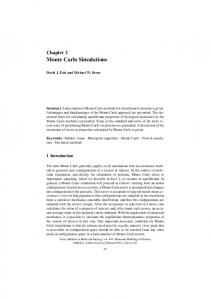
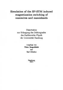
The uncertainty in  is typically 0:2. 3.2. TURNDOWN AGES: STATISTICAL UNCERTAINTIES In Figures 1 and 2, I show LFs computed with mcgolf for the proper motion limit 000 = 0 :0015 yr?1 (parameter set A) and 000 = 0 :0080 yr?1 (parameter set B), respectively. In each Figure, three LFs each are shown for the 4 choices of input age, 7, 10, 13, and 16 Gyr. The numbers of objects in each bin is indicated above the error bars in each case, and the solid lines are the input lfint curves for the same 4 ages. At the left of each curve are 3 numbers. The rst is the age of the input curve in Gyr, the second is Vm , and the third is true. Note that the LF points have been renormalized to the input lfint curves for purposes of display and also because as \observed" samples we would normalize one to the other to determine an age. There are several points of interest in these Figures. First, note that in Figure 1 the 1=Vmax space densities consistently underestimate true by 50%, whereas in Figure 2 the 1=Vmax space densities overestimate true 25% of the time, consistent with the trend tted by Equation 1. Second, note that it is common for pathological objects to cause pronounced \spikes" or \dips" in the LF. These features, if seen in an observed LF, could well be interpreted as re ecting variations in the SFR | the MC results suggest great caution should be used in any detailed interpretation of observed LFs. Third, and related to the previous point, there is signi cant variation in sample-to-sample ages derived by \re- tting" the lfint curves to the MC LFs. The results of these calculations suggest a 1 to 2 Gyr uncertainty in the age determination from sampling statistics alone for 50-object samples, and 0.5 to 1.0 Gyr uncertainty for 200-point samples (not shown). These uncertainties are consistent with the error estimates adopted by LDM and OSWH. Finally, since the statistical variations are most pronounced for bins with N<  5 objects, these results suggest that future observational determinations of the LF would bene t from a binning choice that puts N  5 objects in the lowest-luminosity bin.

MONTE CARLO SIMULATIONS OF THE WDLF

Figure 1.

MC LFs with

5

000 = 0 :00 15 yr?1 . See text.

Acknowledgments: I would like to thank Terry Oswalt for numerous

enlightening discussions. This work was supported by NSF grant AST9217988 and NASA Astrophysics Theory Program grant NAG 5-3103.

4. REFERENCES Bergeron, P., Wesemael, F., and Beauchamp, A. 1995, PASP, 107, 1047 D'Antona, F., & Mazzitelli, I. 1978, A&A, 66, 453 Hernanz, M. Garca-Berro, E., Isern, J., Mochkovitch, R., Segretain, L., & Chabrier, G. 1994, ApJ, 434, 652 Liebert, J., Dahn, C. C., & Monet, D. G. 1988, ApJ, 332, 891

6

MATT A. WOOD

Figure 2.

MC LFs with

000 = 0 :00 80 yr?1 . See text.

Oswalt, T.D., & Smith, J.A. 1995 in White Dwarfs, (Berlin: SpringerVerlag), eds. D.Koester & K.Werner, p. 24 Oswalt, T. D., Smith, J. A., Wood, M. A., & Hintzen, P. M., 1995, Nature, 382, 692 Schmidt, M. 1959, ApJ, 129, 243 Schmidt, M. 1968, ApJ, 151, 393 Winget, D. E., Hansen, C. J., Liebert, J., Van Horn, H. M., Fontaine, G., Nather, R. E., Kepler, S. O., & Lamb, D. Q. 1987, ApJ, 315, L77 Wood, M. A. 1992, ApJ, 386, 539 Wood, M. A. & Oswalt, T. D. 1997, ApJ, submitted. Yuan, J. W. 1992, A&A, 261, 105