MOTE-VIEW: A Sensor Network Monitoring and Management Tool Martin Turon Crossbow Technology, Inc. 4145 N. First Street San Jose, CA 95134 USA
[email protected]
Abstract This paper presents a scalable software framework for managing, monitoring, and visualizing sensor network deployments called MOTE-VIEW. In this paper, we conduct a comprehensive review of typical problems encountered when deploying and administering wireless sensor networks. Then we address these issues by outlining a monitoring tool architecture using an extensible set of user interface components specifically targeted towards improving manageability and easing deployment of wireless sensor networks. We describe specific visualization modules for intuitively characterizing data represented in instantaneous, time span, and spatial form. Next, we will analyze and optimize the database requirements of the proposed visualization modules for performance. Finally, we describe a mechanism for analyzing the health of the individual nodes and the network as a whole.
1. Introduction Wireless sensor networks are a revolutionary, enabling technology, making possible for the first time many novel applications in the fields of environmental monitoring, industrial control, object tracking, and security. Compared to previous methods, the level of resolution and detail that can be gleaned from scattering a large set of tiny, low-power, sensing devices throughout a region is staggering. Despite the exciting possibilities of sensor networks, however, the practical administration of such systems presents clear challenges: 1.
Data volume: The sheer volume of data generated by sensor networks can be tremendous, particularly as the sample rate and number of nodes is increased. Even if the amount of sensor data collected is constrained to the bandwidth limitations of the wireless network, real-time requests for the data can overwhelm the server at the base station if the database queries are not properly designed.
2.
Health monitoring: Each mote, an individual data collection point, is both exposed to the harsh conditions of the environment that surrounds it [1], and limited by the aggressive requirements of maintaining low-power operation to preserve battery life [2]. The network as a whole is designed to withstand the inevitable failure of particular motes [3], but the fragile nature of each mote makes managing the dynamics of network reconfiguration and health evaluation difficult problems.
3.
Information visualization: Presenting and interpreting the voluminous data that are collected presents classic challenges in information visualization.
Therefore, we formulate a framework to directly address issues with managing large sets of sensor data generated by wireless sensor networks. This graphical user interface tool, called MOTE-VIEW, is designed to simplify, from the perspective of the end user, administration of such sensor networks. In particular, we introduce a method to reliably perform calibrated unit conversion of all sensor readings, as well as a set of abstraction layers to allow for extensibility. Our goal is to present the data in a highly usable form, employing effective visualization techniques, whether simple or sophisticated, with a particular emphasis on performance.
2. Background In order to contain failure points within a sensor network system, it is helpful to isolate disparate portions of the system in terms of the software used. Typically, sensor network deployments involve three distinct software tiers: the mote tier, the server tier, and the client tier.
Database
File
Server
Data Access Abstraction Layer
Node Abstraction Layer
Calibration and Unit Conversions
Visualization Abstraction Layer
Figure 2: MOTE-VIEW client-tier abstraction of sensor network data Figure 1: Software used in typical deployments
The mote tier comprises any embedded software that runs on the mote hardware, including a tiny microthreaded operating system (such as TinyOS [6]), firmware applications, and sensor board drivers. Such embedded software is written specifically for the hardware in a language designed for resourceconstrained devices such as nesC, C, or assembly. The server tier provides data logging, database storage, and services for forwarding sensor data coming from the mote gateway. Cross-platform portability is important in the server tier since the hardware may be a PC running Windows or a dedicated appliance running Linux. This portability requirement encourages the use of high-level languages such as Java or C++ within the server tier. The client tier provides a Graphical User Interface (GUI) for managing and visualizing the server and mote tier and is typically designed to run well on an end-user platform of choice: a personal computer or a handheld personal digital assistant (PDA). MOTE-VIEW is a client tier application designed to provide users of wireless sensor networks an interface for end-to-end management and supervision of a deployment. It focuses particularly on solving the three main problems described earlier: data overload, health monitoring, and visualization. The rest of this paper details the design and features of MOTE-VIEW.
3. Architecture Modules within the MOTE-VIEW client are conceptually split into one of four layers. Each of the four layers includes a plug-in capability for providing modular extensions. By mandating a common interface that is extendable with plug-ins, each layer can flexibly scale to support disparate needs within a common framework.
3.1 Data Access Abstraction Layer The MOTE-VIEW client has an interface to abstract and standardize direct access of sensor network data. Such an abstraction is useful because the server tier can provide various sensor network services, or data sources, such as a database of historical readings, a TCP/IP socket providing a live stream of data, or a flat file log. All accesses to sensor network data from client tier modules are done through a Data Access Abstraction Layer (data layer). Each server tier data source has a corresponding driver implemented as a data layer plug-in. By interfacing to the data layer, other MOTE-VIEW modules do not need to know the specifics of how to access the server and can instead make general data-centric requests that get mapped to a particular server service. Initially, data layer calls command an SQL database, specifically via an ODBC (Open Database Connectivity) driver to PostgreSQL, and could be extended to access other services with a plug-in. A database server was chosen over a flat file as the data source for the first version because a database makes random access of the data convenient through SQL, simplifies concurrent connections to the data over TCP/IP, and ably supports large amounts of data.
3.2 Node Status and Configuration Mote platforms are constantly being redesigned, improved, and optimized for particular applications. How to characterize the motes, or nodes, within a sensor network is therefore a logical place to build another layer of abstraction. Each node has some metadata, information that is constant for the entire deployment lifetime: name, set of sensors, configuration, and calibration coefficients. All requests for such node-specific information are made through this Node Abstraction Layer (node layer) and not directly to the database. The node layer is updated upon successful connection to a new database and is
refreshed by any update events sent from the data layer. User-defined mote parameter settings, such as radio frequency and power selection, sample rate, and custom calibration, are configured by interfacing to the node layer. The node layer is also used to cache the latest results from each node. Plug-in modularity at this layer provides support for new sensor boards and mote platforms. A new node layer module, for example, could expose an interface for selecting channels for external probes or setting the excitation voltage of a data acquisition board. Another suitable application would be altering the list of sensor readings to forward in a data packet. Any user preferences set in the node layer are subsequently forwarded to the mote via the data layer.
3.3 Calibration and Unit Conversion Raw sensor data are typically provided as direct digital readings coming out of an ADC (Analog to Digital Converter). The analog voltage of the sensor is sampled and converted to a number relative to some reference voltage. To make the data useful, it is important that they be calibrated and converted to engineering units. Because users will have different preferences as to what final units they prefer, all requests for actual sensor readings are done via a Conversion Abstraction Layer (conversion layer). Drawing from experience working with various sensors, we have found that proper conversion of readings requires: • The ADC reading from the sensor • Calibration coefficients for the sensor • Values for any other dependant variables The conversion layer uses calibration coefficients from the node layer and raw data readings from the data layer to calculate and return final readings in engineering units. All conversion routines belong to this layer. As with the other layers, the conversion layer provides the capability to add extension modules through a plug-in architecture. Such modules supply a library of conversion equations to handle new unit types. Unit conversion functions take the general form of
ystd = F(ADC, c0, …, cn, d0, …, dn) yeng = G(ystd, ueng) where ADC is the raw reading from the sensor, ci is the set of calibration coefficients, and di is the set of dependant variables. Common dependant variables are temperature and voltage. Because converting between different engineering units is straightforward, and converting from raw ADC to engineering units can be complex, the conversion is split into two functions: F and G. F supplies a result in standard international units, which, in the case of temperature would be
degrees Celsius. G then converts that value to userpreferred engineering units (enumerated by ueng) such as Kelvin or degrees Fahrenheit. G functions are implemented for all unit groups, including temperature, pressure, and acceleration; F functions are specific to particular sensor components, including those manufactured by Sensirion and Intersema.
3.4 Graphical Visualization of Wireless Sensor Networks Many users will interface with the sensor network through a textual and graphical display of sensory and link quality data. MOTE-VIEW initially focuses on three representations: (1) instantaneous data points, (2) plots over a span of time, and (3) spatial maps at an instant in time. These different representations are implemented as (1) a spreadsheet, (2) a twodimensional chart with time as the abscissa, and (3) a network topology map respectively. These three visualizations are just a small subset of the possible ways to view data provided by a sensor network. Each of the three visualizations has similarities in the way it interacts with the lower layers of MOTE-VIEW. This overlap is made explicit in a Visualization Abstraction Layer (visualization layer) and is used to form a general plug-in architecture for extending or creating new visualization tools that can be added to MOTE-VIEW. These visualization plug-ins facilitate the extension of MOTE-VIEW’s initial set of text and graphical user interfaces. View Name Data
Description Spreadsheet view of most recent sensor readings from each node Chart Time span plot of a specific sensor over a selected set of nodes Topology Overhead view of nodes in a deployment with network links. Figure 3: Table of initial visualization modules with MOTE-VIEW
The visualization layer also abstracts the concept of time such that it can be controlled by the user. Although the data layer is normally in a real-time or “live” mode, the user may opt to decouple the graphical visualization from the current moment and browse through historical data in a temporal context. This option is provided using a “time bar” component. The time bar supplies a scroll bar and a set of playback controls that link into and command the data grid, chart, and topology. It allows the user to scroll the views back and forth within the time domain and create animated movies of the data.
A good wireless sensor network monitoring tool needs to perform well in three principle ways. First, it needs to be responsive and sift through the data quickly. Second, it must provide a meaningful assessment of the health and status of the network. Third, it must make data from the sensor network available to the user and present that information in the most effective and functional way possible. In this section we evaluate the performance of MOTE-VIEW according to these criteria. In cases where we have found performance limitations, we discuss possible solutions and future directions.
4.1 Database Performance Efficient database retrieval is a critical component of any sensor network visualization tool. Because of long data collection periods and the large number of sample points, the volume of data can grow large. Users tend to expect a monitoring tool to respond instantaneously, however, because the update interval of the network is often set to be slow for power efficiency. Proper caching and indexing is therefore crucial. Sensor network database problems tend to be temporal in nature due to the inherent importance of coupling a sensor reading with the time it was taken. There are three database queries that have been identified as critical to the performance of sensor network visualization problems: 1) What is the last reading from each unique node? 2) What are all the readings from a subset of nodes? 3) What are the node readings in a given time range? Query 3: This query is useful for charting and creating movies of sensor data readings over time. An effective way to speed up such a query is to create a binary tree index tied to the time field of this data. However, a time range query will not indicate whether a node has ever reported, thus necessitating the need for Query 1 to quickly determine the last reading from each unique node. Query 2: This query is primarily used for charting. Indexing the data by node ID can speed up this query, but use of such an index tends to be fragile to the database optimizer logic and only speeds up the operation by a limited amount. To achieve more significant improvements, a subset of random samples can be used instead. Depending on the resolution of the sampling, the operation time can be substantially improved. Moreover, this speed improvement may be
achieved at no cost since the number of data points required is often limited by the number of screen pixels rather than the total number of data points. Query 1: This query is used to populate the node list and for live updates of the data grid and topology map: SELECT DISTINCT ON (nodeid) * FROM result_table ORDER BY nodeid, result_time DESC;
Though such a query should theoretically be sped up by a time-based index, some database engine optimizers do not use the index even when it was available. Completion time for such a query therefore results in being O(n) with respect to the number of records and corresponds closely to the time required to draw all records from the results table (see Figure 3.) In solving this problem, a caching technique proves essential. Instead of forcing the user to wait minutes to open or update the monitoring application, a last results table is created, which takes only 20ms to read. The onus is on the server-side data logger to populate and update this table. An SQL rule is added to do this automatically on every insert by the data logger: CREATE RULE last_result_table AS ON INSERT TO result_table DO ( DELETE FROM last_result_table WHERE nodeid = NEW.nodeid; INSERT INTO last_result_table VALUES ( NEW.* ); ); Query Time vs. Data Size Data (Days)
1 4 7 10 13 16 19 22 25 28 31 34 37 40 43 46 49 52 55 100 Query Time (sec)
4. Performance Analysis
10
1
0.1 0.01
4 nodes every 16 sec 8 nodes every 180 sec 25 nodes every 150 sec 100 nodes every 180 sec
Figure 4: Database access time required to determine last reading from all unique nodes
4.2 Health Monitoring Mechanisms to track the health and status of individual nodes and the network as a whole are considered an essential component of real-world deployments [4]. MOTE-VIEW provides a simple yet effective framework for gleaning a first-order estimate of the reliability of a node. The last reading received
from an individual node is subtracted from the current server time to calculate a health metric called freshness. For example, if no readings from a node have been received for 60 minutes, the color of the node on the display erodes from green to orange to signify that the readings are stale. This technique works remarkably well for locating nodes that have gone offline. Color coding the health of a node also can be used for other metrics: Formula now – result_time # received / # unique sends (seq_no)
current voltage level in the data packet is an easy way to provide an instantaneous view of the battery level and can be invaluable for tracking the root cause of node failure. A more sophisticated and accurate means of estimating node lifetime is to track the amount of time the node has been on. By profiling the time the node is awake in various states and coupling that data with estimates of the current draw of those states, amp·hour estimates can be achieved that correlate highly with actual measurement. Such an integrated current calculation is exactly what is needed to display a power meter for each mote. Unfortunately, such battery characterization requires detailed analysis and customization of the firmware, but this is a worthwhile step for important or expensive deployments. At least one TinyOS application, Surge_TimeSync, outfitted with such a power monitoring technique is currently available.
Name Freshness
Description Time since last result
Success/Yield
% data packets received at base station (not including retries)
Throughput
% data packets received at base station (including retries)
# received / (seq_no + retries)
Quality
Estimate of radio link reliability
Bandwidth
# successful packets over time interval of one second
WMEWMA [5] or avg. throughput to parent 1 sec ∑ receivedi t=0
Congestion
Measure of bottlenecks within the network
Bandwidth / Channel Capacity
Performance of the visualization layer tends to be database limited. While advanced graphical methods can take time, limits in screen resolution provide a natural maximum to the number of data that can be represented. Charting speed is a good example of this phenomenon. By plotting a thinned sample of the data within a desired time span, the charting speed is improved by a factor relative to the inverse of the thinning factor. For instance, plotting 10 percent of the data results in a 10x speed up.
Fairness [3]
Estimate of how well channel capacity is shared
Var(Throughput) Var(Bandwidth)
4.5 Promising Visualization Techniques
4.4 Graphical Performance
Figure 5: Table of useful metrics for determining network health
A detailed description and analysis of the wide variety of possible network health metrics is beyond the scope of this paper. However, many such metrics are available and essential for proper real-time evaluation of the health of a network. Not only is careful selection and construction of such metrics important, but so is the way the information is presented to the user so as to maximize its efficacy for health monitoring.
4.3 Battery Life Characterization The ability to accurately estimate the expected lifetime of a mote is highly desirable. By building good models of battery behavior and characterizing the energy use of particular firmware applications, longterm monitoring networks can be deployed with greater confidence and less administration. Including the
Currently the scale of deployments tends to be in the hundreds of nodes with recent projects, most notably the DARPA eXtreme Scaling Mote (XSM) project, pushing into the thousands [7]. However, when the number of nodes exceeds a few hundred, current visualization paradigms quickly break down. Fortunately, this problem has arisen in other fields, and the research community has devised a rich set of techniques for addressing large, complex datasets. In this section, we explore and evaluate visualization methods that map well to the sensor network domain. When dealing with large numbers of nodes, presentation techniques such as data grids, node lists, and topology maps become overwhelmed. Imagine scrolling through a node list or data grid of more than 10,000 nodes. One method of managing this plethora is to build interfaces for dividing the deployment into logical or regional sets and to visualize details of one such set of nodes either individually, or as an aggregate displayed against other aggregates.
View Name Aggregate Columns [9]
Description Topology view is displayed as a flat plane in 3D. Vertical columns are drawn at each node location with height linked to sensor value. A zoom-in feature provides detailed analysis. Columns are aggregated for close proximity nodes when zooming out. Calendar A 3D chart with sensor value on z-axis, Charting [10] time within day on y-axis, and actual day on x-axis. Provides a mountain range overview of daily trends. Graphic Displays a grid of visualizations rendered Spreadsheets at different times. For example, a 3x3 [11] view of topology over two months would provide a quick comparison of weekly network reformation trends. Node Dome Displays a 3D hemisphere overlaid with [12] the parenting tree of the network. The ball can be rotated and morphed to zoom in on a region. Provides intuitive group selection for deployments of more than 10,000 nodes. Figure 6: Table of promising future visualization modules
5. Discussion In this section, we present a scenario in which a wireless sensor network is employed and show how MOTE-VIEW is used to achieve the objectives of the deployment. The goal is to create a system for detecting intrusions to hazardous areas. Intrusion detection is, in many ways, a perfect fit for wireless sensor technologies. By ubiquitously placing nodes that can sense a local intrusion and linking them together in a network, the entire area becomes suddenly aware of anything that trespasses through it. To fully achieve this goal, the mote needs to be equipped with sensors that suit the task. The XSM600CA intrusion detection mote by Crossbow Technologies is specifically designed for this role. This particular hardware platform has four Passive Infrared (PIR) sensors placed on four sides of the board, a magnetometer, and a microphone. The four PIR sensors detect the motion of a human within 20 feet and a vehicle within 40 feet. The magnetometer detects the movement of metallic objects and is used to discern between humans and vehicles. The microphone provides detection of acoustic triggers.
5.1 Benefits of Modular Visualization Design By creating an extensible architecture, MOTEVIEW can easily be modified for vertical market opportunities or custom projects. One example of this is used with a custom version of the XSM600CA
intrusion detection mote, which has been modified to add quadrant detection circuitry for discerning which combination of the four PIRs triggered a detection event. The topology view of MOTE-VIEW was extended to display the actual quadrants that fire in real-time. Also, because thermal air currents tend to trigger false detections on the PIRs, a simple aggregation algorithm was added to validate detection events only when a corresponding event is seen by at least one neighbor node within a short time window. False positives are depicted as hollowed out wedges, whereas a validated event is drawn as a solid orange wedge in the direction of each quadrant that fired. This extended topology view, customized for a network of XSM600 motes, is then used to monitor the real-time movements of humans and vehicles through a simulated hazardous area. The motes are placed in a grid, 40 feet apart within a column, with the columns 20 feet apart and staggered so the motes are also 40 feet apart within a row (see Fig. 7). MOTE-VIEW is running on a tablet PC and provides updated views of the state of the network every second. The correlation between the display and the real-life events is impressive. A car driving through the area lights up the display in a way that corresponds visibly with its actual path.
Figure 7: MOTE-VIEW display of XSM600 sensor network detecting vehicle intrusion in a parking lot test. PIR triggers are depicted with an orange wedge for each quadrant, and magnetometer triggers are depicted with red node coloring.
References
Figure 8: IsoBar display of light data in MOTE-VIEW
5.2 Heterogeneous Deployment Challenges The issues with increasing the density of deployments, which we described earlier, are compounded when disparate node types are deployed outfitted with different sensors. Therefore, it becomes increasingly important in managing such heterogeneous sensor networks that software tools handle incoming data in a general and intuitive way. By mixing nodes with disparate sets of sensors within the same network, several complications arise. First, the packet format of the various nodes cannot be the same. Because sensor networks use low bandwidth transfers, the amount of data within a data packet is often limited to those sensors with which a given node is equipped. Second, a fixed schema for the results table is no longer sufficient.
6. Conclusion Managing and monitoring wireless sensor networks presents a variety of challenges. Modular design will be key to allow solutions to scale flexibly with the inevitable growth such networks will experience in the future. In conclusion, the MOTE-VIEW framework provides a sound basis for addressing many such challenges.
Acknowledgments Much thanks to Mike Horton, Alan Broad, John Suh and all the early adopters of MOTE-VIEW at Crossbow Technologies for their support of this work. The assistance of Alan Mainwaring and Wei Hong of Intel Research was also greatly appreciated. Finally, Meghan Ward deserves everlasting gratitude for her editing care.
[1] R. Szewczyk, J. Polastre, A. Mainwaring, D. Culler. Lessons from a Sensor Network Expedition. In Proceedings of the 1st European Workshop on Wireless Sensor Networks (EWSN), Jan. 2004 [2] D.Culler, J. Hill, P. Buonadonna, R. Szewczyk, A. Woo. A Network-Centric Approach to Embedded Software for Tiny Devices. In First International Workshop on Embedded Software (EMSOFT), Oct. 2001 [3] A.Woo, T.Tong, D. Culler. Taming the Underlying Challenges of Reliable Multihop Routing in Sensor Networks. In SenSys, Nov. 2003 [4] A. Mainwaring, J. Polastre, R. Szewczyk, D. Culler, J. Anderson. Wireless Sensor Networks for Habitat Monitoring. In Proceedings of the 1st ACM International Workshop on Wireless Sensor Networks and Applications (WSNA), Sep, 2002 [5] A. Woo, D. Culler. Evaluation of Efficient Link Quality Estimators for Low-Power Wireless Networks. [6] J.Hill, R. Szewczyk, A. Woo, S. Hollar, D. Culler, K. Pister. System Architecture Directions for Networked Sensors. [7] J. Suh, M. Horton. Current Hardware and Software Technology for Sensor Networks. In 1st International Workshop on Networked Sensing Systems (INNS), June 2004 [8] J. Hill, M. Horton, R. Kling, L. Krishnamurthy. The Platforms Enabling Wireless Sensor Networks. In review for CACM, Jan. 2004 [9] J. Rayson. Aggregate Towers: Scale Sensitive Visualization and Decluttering of Geospacial Data. IEEE, 1999 [10] J. Wijk, E. Selow. Cluster and Calendar based Visualization of Time Series Data. IEEE, 1999 [11] E. Chi, S. Card. Sensemaking of Evolving Web Sites Using Visualization Spreadsheets. IEEE, 1999 [12] P. Buonadonna, D. Gay, J. Hellerstein, W. Hong, S. Madden. TASK: Sensor Network in a Box. IRB-TR-04021, Jan 2005 [13] O. Staadt, B. Hamann, O. Kreylos, V. Szudziejka. Visualization of Sensor Networks and Sensor Data. In Center for Information Technology Research in the Interest of Society (CITRIS), June 2004 [14] J. Hellerstein, W. Hong, S. Madden, K. Stanek. Beyond Average: Toward Sophisticated Sensing with Queries. In 2nd International Symposium of Information Processing in Sensor Networks (IPSN) Apr. 2003 [15] J. Burrell, T. Brooke, R. Beckwith. Vineyard Computing: Sensor Networks in Agricultural Production. IEEE Pervasive Computing Vol. 3 No. 1, Jan 2004