moving rigid parts, for example pieces of furniture, adjustable screens, doors, etc. A dense 3D reconstruction together with a dense segmentation of the scene ...
Multi-Body Depth-Map Fusion with Non-Intersection Constraints Bastien Jacquet1 , Christian H¨ ane1 , Roland Angst2 , Marc Pollefeys1 1
ETH Z¨ urich, Switzerland 2 Stanford, USA
Abstract. Depthmap fusion is the problem of computing dense 3D reconstructions from a set of depthmaps. Whereas this problem has received a lot of attention for purely rigid scenes, there is remarkably little prior work for dense reconstructions of scenes consisting of several moving rigid bodies or parts. This paper therefore explores this multibody depthmap fusion problem. A first observation in the multi-body setting is that when treated naively, ghosting artifacts will emerge, ie. the same part will be reconstructed multiple times at different positions. We therefore introduce non-intersection constraints which resolve these issues: at any point in time, a point in space can only be occupied by at most one part. Interestingly enough, these constraints can be expressed as linear inequalities and as such define a convex set. We therefore propose to phrase the multi-body depthmap fusion problem in a convex voxel labeling framework. Experimental evaluation shows that our approach succeeds in computing artifact-free dense reconstructions of the individual parts with a minimal overhead due to the non-intersection constraints. Keywords: Multi-view stereo, multi-body structure-from-motion, depthmap fusion, convex optimization, Dynamic Scene Dense 3D Reconstruction
1
Introduction
While there exists a large body of work for rigid multi-view stereo and depth-map fusion methods, there is remarkably little prior work for dense, entirely imagebased 3D reconstructions of multi-body scenes where multiple rigid parts move with different transformations between two frames. However, this is a highly relevant setting since many man-made scenes or objects actually contain multiple moving rigid parts, for example pieces of furniture, adjustable screens, doors, etc. A dense 3D reconstruction together with a dense segmentation of the scene into functional parts is interesting for applications where a user can interact with the reconstructed objects, eg. by opening a door or by pulling out a drawer. This paper therefore addresses this multi-body depth-map fusion problem, and as a byproduct also provides a dense segmentation into differently moving parts. We note that sparse multi-body structure-from-motion (SfM) has received some attention in previous work, see eg. [1]. Since our paper clearly focuses on the dense reconstruction, which requires known camera poses, we assume that those
2
B. Jacquet, C. H¨ ane, R. Angst, M. Pollefeys
Keyboard
Screen
frontal view
frontal view
side view
side view
Input Proposed approach with Depth maps Independent reconstructions images non-intersection constraints Fig. 1: In multi-body depth-map fusion, we are trying to compute a dense reconstruction from a set of input depth-maps of a scene containing multiple moving rigid objects or parts (in the visualized example, the screen rotates w.r.t. the keyboard). A straightforward approach which treats the reconstruction of each rigid part independently leads to severe artifacts, like a part being reconstructed multiple times at slightly different poses (especially visible in the side view where features of the desk, keyboard, and screen get reconstructed multiple times). The approach proposed in this paper introduces non-intersection constraints which enable complex interactions between the individual reconstruction problems thereby eliminating almost all those artifacts.
camera poses are provided by such a sparse multi-body SfM component. For the sake of completeness, we will nonetheless highlight several particular issues with the sparse multi-body setting in Sec. 4. Our multi-body depth-map fusion algorithm only requires depth-maps and camera poses registered to a common references frame. Recent depth-cameras could therefore be used as well, even though in this paper we only consider depth-maps computed from RGB images. As described in detail in Sec. 5, we are building on top of a convex voxel labeling framework for dense rigid reconstructions. In a nutshell, those frameworks label a voxel as either ’occupied’ or ’freespace’ based on a spatial regularization term together with a data fidelity term derived from depth-maps. Those methods provide accurate results for rigid scenes. As multi-body or articulated scenes are assembled from multiple rigid parts, an intuitive idea is to instantiate a separate voxel grid for each part and solve multiple labeling problems independently. However, this leads to severe ghosting artifacts in the reconstructions: described in more detail in Sec. 3, the same part will be reconstructed multiple times, maybe even in a voxel grid associated to another part (see Fig. 1). In order to prevent this from happening, the grids must be allowed to interact with each other. Indeed, if we consider whether the reconstructions of all the parts are intersection free, we see that ghosting artifacts actually lead to intersections with other parts. Hence, our physically-motivated method is based on a remarkably simple, yet powerful idea: a moving rigid part can not occupy a point in space which is already occupied by another rigid part. These non-intersection constraints can be formulated as linear inequality constraints which link the
Multi-Body Depth-Map Fusion with Non-Intersection Constraints
previously independent labeling problems together. This results in complex interactions of regularization and data terms between different grids and will resolve the ghosting artifacts. It is important to note that despite rather weak data terms due to noisy depth maps, the non-intersection constraints result in a strong mutual exclusion principle which provides a clear part-based 3D segmentation. Interestingly, those non-intersection constraint also enable to ’carve out’ regions which have never been directly observed in the input images. For example, observing how a drawer moves in and out of the drawer casing together with the non-intersection constraints immediately lead to the conclusion that the drawer casing must be hollow, a fact which is reproduced by our algorithm. In contrast to previous convex depth-map fusion formulations for rigid scenes, our formulation contains two entirely different types of constraints: the nonintersection constraints and the standard variational formulation of the total variation regularizer. In order to efficiently handle this large optimization problem, we propose to use a preconditioned primal-dual proximal method [2]. Moreover, the set of non-intersection constraints can be quite large. Fortunately, only a small fraction of those constraints will be active at the globally optimal solution, lending itself to an efficient constraint generation procedure. An experimental evaluation shows that our algorithm achieves its goals of a dense multi-body reconstruction. In summary, the contributions of this paper are: i) Introduction of the problem of dense consistent multi-body depth-map fusion and presentation of a solution based on convex non-intersection constraints which not only prevents ghosting artifacts but also carves out voxels in unseen regions which are occupied by another part. ii) Description of a convex voxel labeling algorithm which is solved with a preconditioned primal-dual proximal method and with an efficient constraint generation procedure.
2
Related Work
Image based 3D reconstruction methods have made large progress in recent years. Structure-from-motion (SfM) [3] is nowadays a well-established technique to accurately compute camera poses and sparse 3D point clouds. While originally assuming an entirely rigid scene, sparse 3D reconstruction methods have been extended to deal with multiple rigid bodies [1] or with articulated objects [4,5], and even to more general non-rigidly deforming objects [6,7]. Each of those classes of objects or scenes comes with its own challenges. For example, finding a globally consistent scale for all the objects in a multi-body rigid scene is a non-trivial task, for which no solution exists in the most general case of entirely independently moving rigid objects [8]. Notably, parts of an articulated rigid objects are not allowed to move freely, a fact which manifests itself for example in a rankconstraint for a feature trajectory matrix which can be used to infer joint locations and a global scale [9]. In order to constrain the solution space, reconstruction methods for deformable objects require a prior for regularization, such as local rigidity [10], physically-inspired models [11], or a low-dimensional subspace model
3
4
B. Jacquet, C. H¨ ane, R. Angst, M. Pollefeys
[12]. Even though non-rigidly deformable objects certainly represent an important class of objects, in this paper we focus on reconstructing multi-body rigid and articulated scenes, mainly because these scenes can be broken down into multiple moving rigid parts, whose interaction with each other can be captured in a mathematically exact way, as will be described later. For multi-body rigid scenes, recent efforts in multi-body structure-from-motion led to the simultaneous computation of motion, segmentation and depth-maps from images [13,14]. These approaches estimate the different incremental motions from video with an iterative alternating scheme, and output a single [14] or a sequence [13] of depth-maps, with a segmentation mask and the associated motion for each object. One could feed those into a separate per-object depth-map fusion. However, deferring a reasoning in 3D can lead to ghosting artifacts where parts intersect or get reconstructed multiple times. This happens when a part remains photoconsistent w.r.t. another part, eg. for object shadows on the ground plane, as can be seen in [13,14]’s results. Our goal differs from theirs as we aim at volumetric, non-intersecting and time-consistent 3D models from unordered depth-maps. [13,14] can therefore be used to generate input depth-maps for our method. In the Computer Graphics community, Chang and Zwicker’s work [15] also addresses the problem of registering data from an articulated object in different configurations, mainly in order to infer the articulation chain and the assignment of points to parts. However, their focus differs from ours: while we are interested in a dense volumetric reconstruction from image data, their approach requires high-quality outlier-free point clouds as input so that no optimization over the 3D locations of the points is required. Unfortunately, image based methods require a SfM stage and point clouds acquired by SfM techniques tend to be very noisy and contaminated with many outliers, the same being true for RGBD-sensors. Those outliers are not handled by their method. Moreover, non-intersection constraints are not considered at all in [15]. Once camera poses are known from a sparse reconstruction method, dense reconstruction algorithms can be used to compute and extract 3D surfaces. Also known as multi-view stereo, this field contains a large amount of previous work. We refer the reader to [16] and its excellent accompanying website for further related work in this area. Carving out regions in 3D which project to non-occupied areas in the images have lead to the well-understood concept of the visual-hull [17]. Phrasing the multi-view stereo problem as a binary labeling problem of a 3D voxel grid with labels ’occupied’ or ’freespace’ and adding regularization, [18] has used graph-cuts to optimize the resulting energy minimization problem. Shortly after that, this discrete graph-cut formulation has been rephrased in the continuous setting as a convex optimization problem [19], where an efficient, highly parallelizable algorithm has been introduced. More generally, convex relaxations of binary or multi-label problems can be used to combine data evidence from images with a regularization term, usually a total-variation term, in an efficient, highly parallelizable framework [20]. Our multi-body depth-map fusion approach builds on top of such convex relaxations. Recent approaches with RGBD cameras
Multi-Body Depth-Map Fusion with Non-Intersection Constraints Input Images
Motion Multi-Graph
Depthmaps Part 1
Sparse MultiBody SfM
Subgraph Extraction
First Stage
Dense IntersectionFree Reconstruction
Part 2
Convex Depthmap Fusion Second Stage
Fig. 2: The overall dense reconstruction pipeline takes an unordered set of images as input. As a preliminary stage, a sparse multi-body SfM component extracts a motion multigraph: a node represents an image and each edge represents a relative rigid transformation (of the camera or a rigid part) between two images. After selecting the appropriate subgraph for each part, depthmaps can be computed for that part. In the main stage, those depthmaps are fused in a volumetric convex voxel labeling framework where each part is reconstructed in a separate voxel grid. However, non-intersection constraints between the parts enable a complex interaction between all those grids, thereby carving out voxels in unseen areas which are occupied by another part and avoiding reconstruction artifacts such as ’ghost parts’.
[21] only consider the unary data term and ignore any pairwise or higher-order regularization term, thereby sacrificing accuracy in favour of speed. Such a fusion approach has recently been extended for articulated model-based tracking [22]. Analogously to our approach, the model is represented by instantiating a separate voxel grid for each rigid part. An iterative-closest point algorithm between a new RGBD frame and the model is used to update the camera position, and given this camera position the new data evidence is fused into the grids. Hence in direct comparison to our approach, [22] is much faster but also less accurate, ignores the physical non-intersection constraints, and requires a RGB-D camera together with a continuous stream of images for incremental computation.
3
Problem Description and System Overview
The input to our algorithm consists of a set of depth-maps taken from a scene with multiple moving rigid objects or parts. Furthermore, the camera is also allowed to move. The number of parts G is assumed to be known. Our reconstruction pipeline contains a preliminary depth-map generation stage, and a main fusion stage, see Fig. 2. The depth-map fusion stage is based on a volumetric fusion of depth-maps in a voxel grid. In contrast to previous approaches which consider a single rigid object and thus only a single voxel grid, we propose to use a separate voxel grid for each part in order to tackle the dense multi-body depth-map fusion problem. This second stage will be described in detail in Sec. 5. As we will see, in order to define a data term for a certain image and part, the depth-maps must be registered to those voxel grids, each of which is rigidly attached to a part. This registration step obviously requires the camera position of this depth-map with respect to that part. The preliminary
5
6
B. Jacquet, C. H¨ ane, R. Angst, M. Pollefeys
stage (outlined in Sec. 4) therefore performs a multi-body sparse reconstruction in order to compute all the camera poses and the motions of the parts. Once all the camera poses are known, depth-maps can be generated to be used in the main fusion stage. At this point it is important to highlight a problem particular to the multibody setting. Let us consider a simple setup with two parts and look at sets of depth-maps generated in two different cases. In the first case, the two parts move with respect to each other between any two images. The resulting depth-maps for each part will contain highly confident measurements in regions where that part is visible and contain random measurements with low confidence in regions of the other part because the motions of the two parts are different and thus inconsistent for computing a single depth-map. In the second case however, only the camera moves and the two parts stay rigid with respect to each other. The depth-maps for those images will be the same for both parts and contain highly confident measurements for both parts. Fusing all those depth-maps from the first and second case for each part independently will lead to ghost parts: the highly confident measurements of the second case provide consistent evidence for both parts in each one of the two voxel grids, whereas the inconsistent regions with low confidence in depth-maps of the first case would be simply treated as outlying measurements for example due to occlusions. In summary, the two parts would get reconstructed in both voxel grids leading to ghost parts which would occupy the same points in space once a voxel in one grid is mapped to the other grid. Therefore, our proposed fusion process allows the grids to interact with each other in a complex way so that parts are guaranteed to not intersect with each other at any point in time. This does not only avoid ghost parts, it also allows to carve out regions in space which have never been observed directly in any of the images.
4
Sparse Multi-Body Structure-from-Motion
As mentioned in the introduction, the main contribution of this paper is the dense depth-map fusion formulation with non-intersection constraints. To compute the required camera poses, iterative approaches similar to those used in [13,14] could be used. We preferred a non-iterative one that we quickly outline in this section explain, for the sake of completeness. This first stage mostly uses existing building blocks for sparse multi-body SfM. 4.1
Extracting Relative Transformations
Since each part is allowed to move with respect to other parts and the camera, we initially treat the reconstruction of each part as a separate rigid SfM problem. Sparse feature point correspondences are therefore fed into a sequential RANSAC which extracts all the essential matrices with sufficient inlier support. While being a fairly simple and straight-forward approach, sequential RANSAC has
Multi-Body Depth-Map Fusion with Non-Intersection Constraints
proven to be sufficient for our purposes. As two-view epipolar geometry might lead to many spurious inliers (eg. due to repetitive structure), a three-view verification is performed to eliminate inaccurately detected essential matrices. An additional benefit of three-view verification is that the scale for relative transformations within a three-view verified cluster of images is fixed (two-view relations only provide the translation up to scale) and a consisten reference coordinate frame can be chosen for this cluster. It is important to note that such a cluster can nonetheless contain relative transformations from multiple different parts: Whenever two parts do not move with respect to each other between two images (as visualized by the dashed arrow in Fig. 2), their threeview verified relative transformations which link to those two images will be assigned to the same cluster thereby fixing a consistent scale between the two parts. If a part is never static with respect to another part, additional heuristics such as a common ground plane or motion constraints can be used [8,23]. For simplicity, we decided to take two pictures with a moving camera where no part is moving. This provides a common reference frame and scale for all the relative transformations. Conceptually, at this point, a multigraph with a node for each image and an oriented edge for each extracted relative rigid transformation captures the geometric relations between the images.
4.2
Motion Segmentation
In order to get the rigid motion of part g, the correct subset of edges needs to be selected from the multigraph. Note that an edge can be selected multiple times: this happens if two or more parts do not move with respect to each other between two images. This is a special instance of the motion segmentation problem for which a fair amount of previous work exists [1,24,5,8,13,14]. If a feature point on a certain part can be tracked throughout all the images, the motion segmentation becomes trivial for that part. If this is not the case, heuristics based on color similarity, spatial proximity, etc. can be used to ’stitch’ partial feature trajectories together and read off the correct segmentation from the result. Since motion segmentation is not the focus of our work, we ask for user input to manually correct erroneously stitched trajectories. Interestingly, the dense reconstruction framework can handle some potential errors in the motion segmentation. This robustness is mainly due to the following observations. (i) Each subgraph is built from robust, three-view verified relations because the original multigraph is built that way as well. The motion subgraph for part g is further refined by running a rigid bundle adjustment on that subgraph. This further eliminates wrongly included or inaccuratly estimated relative transformations. (ii) Remaining inaccurately registered views in a subgraph will be handled by two components in our framework: Firstly, inaccurate views lead to depthmaps with low confidence scores and hence they will contribute less to the data term. Secondly, the depth map fusion algorithm uses a robust data cost and a regularization term which inhibit outlying measurements to some extent.
7
8
4.3
B. Jacquet, C. H¨ ane, R. Angst, M. Pollefeys
Generating Cost Volumes
Once the subgraph and thus relative transformations for each part is known, depthmaps for that part can be generated for each node (ie. camera view) in the subgraph. We are currently using a CUDA-implemented plane-sweep algorithm similar to [25] for the computation of the depth maps. The depth maps of a specific part g are all registered into a separate cost volume for that part. Specifically, given the positions of the grid g and camera, each depth map is converted into a truncated signed distance field and these values are aggregated in a voxel grid dg . The contribution to the signed distance field of a depth measurement at a certain pixel in a depthmap is weighted with a pixel confidence score based on the disparity matching cost for that pixel. These voxel grids are then used as data evidence in the dense reconstruction step. The orientation and extents of the voxel grid for a part are given by a well-aligned and tightly fitted bounding box around the sparse point cloud associated to that part. This bounding box is robustly estimated by considering the distributions of the projection of this point cloud onto normal directions of dominant scene planes contained in that point cloud. Note that in this way, the grids are best aligned with respect to each part and are not axis-aligned to each other.
5 5.1
Dense Multi-Body Depth-Map Fusion Preconditioned Primal-Dual Proximal Method
Continuous Formulation Motivated by widely-used convex formulations for binary segmentation problems [19,20], our formulation is based on a separate ’occupancy indicator function’ xg ∶ Vg → [0, 1] for each grid g ∈ {1, . . . , G}. Vg denotes a spatial volume around part g and a value of xg (v) = 1 denotes that this point v ∈ Vg is occupied by part g whereas xg (v) = 0 denotes unoccupied freespace. The local data evidence dg (xg ) from the depth maps is combined with a regularization term rg (xg ) in a continuous energy function. Specifically, we follow a convex fusion framework with the widely-used total-variation regularization rg (xg ) = ∫Vg ∥∇xg (v)∥dv and a unary data term ⟨dg , xg ⟩ = ∫Vg dg (v)xg (v)dv [19]. Hence, the continuous energy functional looks like E(x) = ∑ rg (xg ) + µ⟨dg , xg ⟩,
(1)
g
where x = {x1 , . . . , xG } denotes the set of occupancy densities and µ ∈ R is a parameter balancing data fidelity with the regularization. For later reference, we note the variational representation of the total-variation ∫Vg ∥∇xg (v)∥dv = maxpg ∶∥pg (v)∥≤1 ∫Vg ⟨pg (v), ∇xg (v)⟩dv, which makes use of a dual vector-valued function pg ∶ Vg → R3 . Since each rigid part g is allowed to move in the scene, the volumes Vg actually move rigidly with respect to each other and thus also with respect to a fixed global coordinate system. The non-intersection constraints impose that at any
Multi-Body Depth-Map Fusion with Non-Intersection Constraints
point in time, no point in space can be occupied by more than one part. Formally, let Tt,g0 →g denote the rigid transformation which maps a point v ∈ Vg0 from grid g0 at time t to the local coordinates of grid g. The transformations Tt,g0 →g are computed as described in Sec. 4. Hence, we have access to transformations at points in time t for which we have image observations. The non-intersection constraints then become ∀v ∈ Vg0 ∶
∑
g∈{1,...,G}
xg (Tt,g0 →g (v)) ≤ 1.
(2)
Note that for known Tt,g0 →g , the non-intersection constraints are linear inequality constraints with respect to the unknown functions xg . This observation is important since this allows us to include those non-intersection constraints in a convex optimization framework.
Discretization In the discrete setting, the volumes Vg are represented by appropriately sized and aligned voxel grids around each part. The set of indices for voxels in grid g is also denoted by Vg , and the number of voxels in grid g equals ng = ∣Vg ∣. xvg ∈ [0, 1] denotes the occupancy indicator of a voxel vg ∈ Vg , whereas xg = (⇓vg ∈Vg xvg ) ∈ [0, 1]ng is the vertical concatenation of labels for voxel grid g. Similarly, the complete vector of occupancy indicator variables is given by x = (⇓g∈G xg ) ∈ [0, 1]∑g ng . An analogous notation is used for dual variables pv and the unary data costs dg . Using the variational form of the total variation, the discrete version of Eq. (1) is E(x) = ∑ ∑ max⟨pvg , ∇xvg ⟩ − i(pvg ≤ 1) + µdvg xvg + i(xvg ∈ [0, 1]), g vg ∈Vg pvg
(3)
where i denotes the indicator function (0 if condition is met, ∞ if not) and ∇xvg is computed with finite forward differences. As we will see in Sec. 5.2, the non-intersection constraints can be represented as a linear inequality Ax ≤ b. After introducing Lagrange multipliers z in order to handle this linear constraint set, the primal-dual formulation of the resulting optimization problem looks like z min max⟨( ) , Kx⟩ − F ∗ (p, z) + G(x), p x p,z
where F ∗ (p, z) = i(p ≤ 1) + ⟨z, b⟩ + i(z ≥ 0) G(x) = µ⟨d, x⟩ + i(x ∈ [0, 1]) K = [AT , ∇ ] . T T
(4) (5) (6) (7)
The function F ∗ (convex conjugate of F ) acts on the dual variables and G on the primal variables and the linear operator K connects these two sets of variables. Here, the sparse matrix ∇ ∈ R3 ∑g ng ×∑g ng contains the finit forward difference coefficients for gradients ∇xvg .
9
10
B. Jacquet, C. H¨ ane, R. Angst, M. Pollefeys
Optimization This is a large-scale convex optimization problem and we need to carefully select a suitable algorithm. We decided to use a first order primaldual proximal algorithm [20,26], mainly because the individual update steps in this algorithm decouple and can be parallelized easily. Experimentally, we have confirmed that a preconditioned proximal algorithm [2] converges much faster than its non-preconditioned counterpart. This is due to the fact that our linear operator K captures two different type of constraints, namely the non-intersection constraints and the constraints due to the variational form of the total variation. Not only contain the matrices A and ∇ a different number of rows, these rows also contain an entirely different pattern of non-zero entries with values on a different order of magnitude. Using a single step-length for all the dual variables as done in a non-preconditioned proximal method can therefore lead to slow convergence. However, as Chambolle and Pock have shown in [2], a preconditioned primal-dual proximal algorithm with a diagonal preconditioner can choose an adaptive step length per variable. For the sake of completeness and since the derivations need some attention, the required prox-steps of F ∗ and G for the preconditioned version will be derived in the following. The preconditioned prox-step replaces the standard L2-norm ∥.∥2 with a Mahalanobis distance ∥.∥Σ , in our case Σ is a diagonal positive-definite matrix. Even though F ∗ decouples into separate prox-steps for p and z, the prox-step for the latter involves a sum between a linear term ⟨z, b⟩ and the indicator function i(z ≥ 0) leading to the following derivation ˜ ∥Σ ) prox⟨⋅,b⟩+i(⋅≥0),Σ (˜ z) = arg min (⟨z, b⟩ + i(z ≥ 0) + ∥z − z 2
(8)
z
˜∥ ) = Σ 2 arg min1 (⟨Σ 2 z′ , b⟩ + i(Σ 2 z′ ≥ 0) + ∥z′ − Σ− 2 z 1
1
z′ =Σ− 2 z
1
1
2 I
˜∥ ) = Σ 2 arg min (⟨z′ , ΣT 2 b⟩ + i(z′ ≥ 0) + ∥z′ − Σ− 2 z ′ 1
1
1
2 I
z
⎧ ⎪ 1 1 1 z − Σb if ˜ z − Σb > 0 ⎪˜ z − ΣT 2 b) = ⎨ . = Σ 2 proxi(⋅≥0),I (Σ− 2 ˜ ⎪ 0 if ˜ z − Σb ≤ 0 ⎪ ⎩
In the second last step, we have used the property that a non-preconditioned 1 prox-step involving a linear term ⟨z′ , ΣT 2 b⟩ is equivalent to applying the prox1 1 step to the difference Σ− 2 ˜ z − ΣT 2 b (see also Table 1 iv in [26]). Since Σ is chosen diagonal, the prox-steps for z still decouple. The derivation for the prox-step of the primal variable follows exactly the same steps and gives ˜ + µTf )). proxµ⟨d,⋅⟩+i(⋅∈[0,1]),T (˜ x) = max(0, min(1, x
(9)
A similar derivation for the dual variable pvg with Σpvg = σv2g I3 provides ⎧ p ˜ ⎪ ⎪ ⎪ ˜ proxi(∥⋅∥≤1),Σvg (˜ p) = ⎨ p ⎪ ⎪ ⎪ ∥˜ p∥2 ⎩
if ∥˜ p∥2 ≤ 1
if ∥˜ p∥2 > 1
,
(10)
Multi-Body Depth-Map Fusion with Non-Intersection Constraints
Algorithm 1: First-Order Primal-Dual Algorithm parameters : Time step sizes τj = m 1 2−α , T = diag (τj ), σi = n 1 α , Σ = diag (σi ), ∑ ∣Ki,j ∣
output 1 2 3 4 5 6 7 8 9 10 11 12
∑ ∣Ki,j ∣
primal-dual step trade-off α ∈ [0, 2] : Minimizer x for the multi-body depth-map fusion problem. i=1
j=1
while not converged do // Primal Variable Update: zt ˜ = xt − TKT ( t ) ; x p // Primal Variable Prox-Step: xt+1 = proxµ⟨d,⋅⟩+i(⋅∈[0,1]),T (˜ x) ; // Reflection step: ˆ = 2xt+1 − xt ; x // Dual Variable Update: ˜ z zt ( ) = ( t ) + ΣKˆ x; ˜ p p zt+1 = proxi(⋅≥0), (˜ z − Σz b) ; p) ; pt+1 = proxi(∥⋅∥≤1),Σp (˜ t=t+1 ;
ie. the preconditioning does not affect this prox-step. In summary, a first-order primal-dual preconditioned proximal algorithm for our non-intersection constrained multi-body depth-map fusion problem looks like outlined in Alg. 11 . Note again that all the prox-steps decompose into elementwise prox-steps which can be solved analytically and in parallel. 5.2
Non-Intersection Constraints as Linear Inequalities
This section derives the discretized linear inequality constraints which enforce the non-intersection constraints. We recall that Tt,g→g′ denotes the rigid transformation from grid (or rigid part) g to g ′ at frame t. Let wt,vg ∩vg′ denote the intersection volume between voxels vg and vg′ at time t. This is computed by applying the rigid transformation Tt,g→g′ to the voxel cube vg ∈ Vg which yields the corresponding translated and rotated cube at time t expressed in coordinates of grid g ′ . Even though there exist efficient and fast algorithms for exact voxel cube intersections [27], we opted for a simple estimation procedure of the intersection volume between two voxels. Inspired by Monte Carlo integration and efficient collision detection procedures from computer graphics, a voxel vg is subdivided into n regularly spaced sample points. Each sample point is transformed into the other grid and a counter nvg′ is increased for the voxel vg′ which 1
The primal-dual trade-off was fixed to α = 1 for all our experiments.
11
12
B. Jacquet, C. H¨ ane, R. Angst, M. Pollefeys
contains the transformed point. The final intersection volume is then estimated as nv ′ wt,vg ∩vg′ ≈ ng . In practice, we used n = 163 sampling points. With this notation in place, the discrete version of the non-intersection constraint in Eq. (2) reads like the following: For each frame t and each voxel v ∈ Vg0 in the grid g0 , it must hold that ∑ ∑ wt,v∩vg xvg ≤ 1. g vg ∈Vg
(11)
Those constraints can be concisely captured in a linear matrix inequality Ax ≤ 1, where the entries of the matrix A are equal to the weights wt,v∩vg . Obviously, some of those constraints are redundant (due to symmetry reasons) and therefore not required. Notably, most of the voxels are not intersecting, hence, most of the weights wt,v∩vg will be zero resulting in a highly sparse matrix. In practice, there are roughly 6.5 non-zero entries per grid in each row of the matrix A. Nevertheless, the overall number of intersection constraints and thus rows in A can be very large. Fortunately, only a very small fraction of those constraints will be active at the globally optimal solution. Therefore, we follow a constraint generation approach in our implementation: after a certain number of iterations, we search for violated constraints and those constraints which are close to becoming violated and add those as additional rows to the constraint matrix. Note that when adding new rows to matrix A, σi and τj need to be updated. The constraint generation procedure can be formulated with a complexity of O(nt ng0 G) where nt denotes the number of images where parts have moved w.r.t. each other. The outermost loop iterates over all time instances t ∈ {1, . . . , nt }. The next loop iterates over all voxels v ∈ Vg0 in a reference grid g0 2 . Again motivated by collision detection procedures in computer graphics, a sequence of increasingly more complex conservative checks are employed in order to determine early on whether constraint [t, v] is not violated and can be skipped. For those checks, potentially intersecting voxels in other grids g ≠ g0 are efficiently computed with integer index arithmetic as neighbor of Tt,g0 →g (v). This constraint generation procedure incurs only a small overhead to the primal-dual method.
6
Results
We present an experimental evaluation on the following datasets and we also refer to the supplemental material for further results: – Laptop: This data set contains 18 images of a laptop where the screen is rotating around its fixed axis w.r.t. the keyboard. The screen is not moving w.r.t. the keyboard in all the frames, ie. in some frames only the camera moved and the scene was perceived as being entirely rigid during those frames. 2
Here, we implicitly assume that grid g0 is sufficiently large so that by iterating over its voxels, all the non-intersection constraints are considered. A better approach would be to use a hierarchical space partitioning scheme to efficiently compute the regions in which voxel grids intersect. However, we leave that for future work.
Multi-Body Depth-Map Fusion with Non-Intersection Constraints
Background and casing
Drawer
Input images
Sample depth maps
Intersection-free reconstruction
Fig. 3: When a drawer moves in and out of the casing, the intersection-constraints automatically carve out a tight hole in the casing in order to avoid any intersections between the drawer and the casing. Moreover, the drawer is reconstructed only once, ie. no ghosting artifacts are present. The visualized depth maps correspond to the input image on the top left. Note that this example only uses 6 input images from one side of the drawer and hence, due to absence of data evidence, the reconstruction on other sides can be inaccurate.
For this example, we have used a best-K (K = 6) depthmap matching cost which is robust to occlusions and, more importantly for our setting, also to changes in the rigid configuration of the two parts. This choice results in depthmaps which are fairly consistent for both parts at the same time. Some of those depthmaps are shown in Fig. 1. We can clearly see that the regions of the screen and keyboard in those depthmaps will both provide consistent data evidence in the keyboard and screen voxel grid. Without any non-intersection constraints, the screen should therefore also be reconstructed in the keyboard grid (and the other way around for the keyboard in the screen grid). As the results show, the screen will indeed be reconstructed multiple times, in our case 6 times since we observed 6 different configurations between the keyboard and the screen. However, with activated non-intersection constraints, those ghosting artifacts vanish and the screen and keyboard will be reconstructed exactly once, each in its own grid. – Drawer: The drawer dataset consists of 6 images. 4 different non-rigid configurations have been observed while pushing the drawer into the drawer casing. Hence, in three images, the scene was again perceived as entirely rigid. In contrast to the laptop example where we have used a best-K depthmap matching, all the views contribute to a depthmap estimate this time. Fig. 3 shows an example of the resulting depthmaps for one specific point of view. Note that even though there is a bias towards either the casing or the drawer, there is a fair amount of noise present in those depthmaps. Nevertheless, our algorithm provides an artifact free reconstruction and thus segmentation into the two parts. Moreover, the non-intersection constraints prevent intersections even in unseen or weakly observed areas, resulting in a tight hole in the casing of the drawer such that the drawer can slide in.
13
14
B. Jacquet, C. H¨ ane, R. Angst, M. Pollefeys
The non-intersection constraints obviously increase the time and memory requirements slightly compared to entirely independent reconstructions. It is difficult to exactly quantify the time overhead due to those constraints, since the additional complexity for the constraint generation largely depends on how many occupied and intersecting voxels there are in a per-part independent reconstruction (and hence on the proximity between the parts). In our experiments, the overall time overhead for the primal-dual algorithm was usually within 25 − 50%. We observed a similar overhead for the memory requirements. We currently do not remove constraints which were added to the constraint matrix at some point and got satisfied later on. Such a step could certainly be added if required.
7
Conclusion and Future Work
In this paper, we have introduced the multi-body depth-map fusion problem. In order to prevent ghosting artifacts, we have considered the non-intersection constraints which can be formalized as linear inequalities. These inequalities have been integrated in a convex voxel labeling framework, leading to complex interactions between separate voxel grids for each rigid part. As the experimental evaluation shows, this approach eliminates ghosting artifacts. Moreover, regions which have never been observed in the images, like the interior of a drawer case, will be carved out if an intersection with another part would result otherwise. Intuitively, a part can be used to carve out unseen regions in other parts. From an optimization point of view, we verified that a preconditioned primal-dual proximal method converges must faster than its non-preconditioned counterpart. This can be attributed to the fact that our optimization problem contains two entirely different types of dual variables, a setting in which preconditioning is known to be beneficial. Since only a small fraction of the intersection constraints will be active at the globally optimal solution, a constraint generation approach has been introduced to handle the large set of non-intersection constraints without incurring a large overhead to the primal-dual method.
Acknowledgments This work has been supported by the Max Planck Center for Visual Computing and Communication, by the 4DVideo ERC Starting Grant Nr. 210806 and by the Swiss National Science Foundation under Project Nr. 143422.
Multi-Body Depth-Map Fusion with Non-Intersection Constraints
References 1. Costeira, J.P., Kanade, T.: A multi-body factorization method for motion analysis. In: ICCV, Washington, DC, USA, IEEE Computer Society (1995) 1071–1076 2. Pock, T., Chambolle, A.: Diagonal preconditioning for first order primal-dual algorithms in convex optimization. In: ICCV, Washington, DC, USA, IEEE Computer Society (2011) 1762–1769 3. Hartley, R., Zisserman, A.: Multiple view geometry in computer vision. 2nd edn. Cambridge University Press (2004) 4. Ross, D.A., Tarlow, D., Zemel, R.S.: Learning articulated structure and motion. IJCV 88(2) (2010) 214–237 5. Katz, D., Brock, O.: Interactive segmentation of articulated objects in 3d. In: Workshop on Mobile Manipulation at ICRA 2011. (2011) 6. Brand, M.: A direct method for 3d factorization of nonrigid motion observed in 2d. In: CVPR, Washington, DC, USA, IEEE Computer Society (2005) 122–128 7. Torresani, L., Hertzmann, A., Bregler, C.: Nonrigid structure-from-motion: Estimating shape and motion with hierarchical priors. IEEE TPAMI 30(5) (2008) 878–892 8. Ozden, K., Schindler, K., Van Gool, L.: Multibody structure-from-motion in practice. IEEE TPAMI 32(6) (2010) 1134–1141 9. Yan, J., Pollefeys, M.: A factorization-based approach for articulated nonrigid shape, motion and kinematic chain recovery from video. IEEE TPAMI 30(5) (2008) 865–877 10. Taylor, J., Jepson, A.D., Kutulakos, K.N.: Non-rigid structure from locally-rigid motion. In: CVPR Computer Society, Washington, DC, USA, IEEE Computer Society (2010) 2761–2768 11. Agudo, A., Calvo, B.n., Montiel, J.M.M.: 3d reconstruction of non-rigid surfaces in real-time using wedge elements. In: ECCV. Lecture Notes in Computer Science, Berlin, Heidelberg, Springer (2012) 113–122 12. Garg, R., Roussos, A., de Agapito, L.: Dense variational reconstruction of nonrigid surfaces from monocular video. In: CVPR, IEEE Computer Society (2013) 1272–1279 13. Zhang, G., Jia, J., Bao, H.: Simultaneous multi-body stereo and segmentation. In: Computer Vision (ICCV), 2011 IEEE International Conference on. (Nov 2011) 826–833 14. Roussos, A., Russell, C., Garg, R., Agapito, L.: Dense multibody motion estimation and reconstruction from a handheld camera. In: Mixed and Augmented Reality (ISMAR), 2012 IEEE International Symposium on. (Nov 2012) 31–40 15. Chang, W., Zwicker, M.: Global registration of dynamic range scans for articulated model reconstruction. ACM Transactions on Graphics 30(3) (May 2011) 26:1–26:15 16. Seitz, S.M., Curless, B., Diebel, J., Scharstein, D., Szeliski, R.: A comparison and evaluation of multi-view stereo reconstruction algorithms. In: CVPR, IEEE Computer Society (2006) 519–528 17. Laurentini, A.: The visual hull concept for silhouette-based image understanding. IEEE TPAMI 16(2) (February 1994) 150–162 18. Lempitsky, V.S., Boykov, Y.: Global optimization for shape fitting. In: CVPR. Volume 7., Washington, DC, USA, IEEE Computer Society (2007) 1–8 19. Zach, C.: Fast and high quality fusion of depth maps. In: 3DPVT 2008, Atlanta, GA, USA June 18 - 20, 2008. (2008)
15
16
B. Jacquet, C. H¨ ane, R. Angst, M. Pollefeys
20. Chambolle, A., Pock, T.: A first-order primal-dual algorithm for convex problems with applications to imaging. Journal of Mathematical Imaging and Vision 40(1) (2011) 120–145 21. Newcombe, R.A., Davison, A.J., Izadi, S., Kohli, P., Hilliges, O., Shotton, J., Molyneaux, D., Hodges, S., Kim, D., Fitzgibbon, A.: Kinectfusion: Real-time dense surface mapping and tracking. In: IEEE Symposium on Mixed and augmented reality (ISMAR), 2011, IEEE (2011) 127–136 22. Malleson, C., Klaudiny, M., Hilton, A., Guillemaut, J.Y.: Single-view rgbd-based reconstruction of dynamic human geometry. In: The IEEE International Conference on Computer Vision (ICCV) Workshops. (June 2013) 23. Jacquet, B., Angst, R., Pollefeys, M.: Articulated and restricted motion subspaces and their signatures. In: Computer Vision and Pattern Recognition (CVPR), 2013 IEEE Conference on, IEEE (2013) 1506–1513 24. Tron, R., Vidal, R.: A benchmark for the comparison of 3-d motion segmentation algorithms. In: CVPR, Washington, DC, USA, IEEE Computer Society (2007) 25. Yang, R., Pollefeys, M.: Multi-resolution real-time stereo on commodity graphics hardware. In: Computer Vision and Pattern Recognition, 2003. Proceedings. 2003 IEEE Computer Society Conference on. Volume 1. (June 2003) I–211–I–217 vol.1 26. Combettes, P.L., Pesquet, J.C.: Proximal Splitting Methods in Signal Processing. ArXiv e-prints (December 2009) 27. Reveill`es, J.P.: The geometry of the intersection of voxel spaces. Electronic Notes in Theoretical Computer Science 46 (2001) 285–308
Multi-Body Depth-Map Fusion with Non-Intersection Constraints: Supplemental Material Bastien Jacquet1 , Christian H¨ ane1 , Roland Angst2 , Marc Pollefeys1 1
ETH Z¨ urich, Switzerland 2 Stanford, USA
Abstract. The supplemental material reports additional results computed with the proposed multi-body depth-map fusion algorithm with non-intersection constraints.
1
Laptop
Here, we report some additional results based on the Laptop dataset. This dataset contains 18 images of a laptop, taken from a moving camera while the screen of the laptop was moving with respect to the keyboard. The data has been captured such that a fixed configuration between the keyboard and screen has only been observed from at most 3 different camera poses. This means for example that for the keyboard grid, the accumulated consistent evidence over all 3 camera poses for a ghost screen is weaker than the evidence for the keyboard which accumulates data from 18 camera poses. In such a situation, an alternative idea to decrease the ghosting artifacts is to put more emphasis on the spatial regularization term, hoping that regions with low evidence won’t get reconstructed due to the otherwise implied high regularization cost. As Fig. 1 shows, such a strategy can indeed decrease the ghosting artifacts to some extent. However, some artifacts remain and the screen still intersects with the keyboard. With our non-intersection constraints, those artifacts and intersections vanish. It is important to note that putting more emphasis on the regularization term can lead to other artifacts, like the elimination of correct regions which are not part of a ghosting artifact or a smooth interpolation between a ghost part and the correct reconstruction (as seen in Fig. 1). Hence, the success of this strategy strongly depends on the motion of the camera and the frequency of changing configurations between the parts.
2
Box
This dataset consists of 13 images taken from a moving camera and a moving wooden box in front of a rigid background. The wooden box translates and rotates which can lead to severe artifacts if not handled properly. We refer to Fig. 2 for some sample input images, depth-maps corresponding to these images for the
2
B. Jacquet, C. H¨ ane, R. Angst, M. Pollefeys
Sample Input images
Sample Depth maps
Without Non-Intersection Constraints
With Non-Intersection Constraints
Fig. 1: In comparison to the results reported in the paper, here we increased the spatial regularization term considerably. This eliminates artifacts to some extend even without non-intersection constraints. However, as the close-up views with a slicing plane show, intersections are still present without non-intersection constraints. Moreover, the background plane has wrongly been interpolated smoothly with the most widely-opened position of the screen. Two artifacts remain in both reconstruction. These are due to inaccuracies in the depthmaps, as can be seen in some of the visualized sample depthmaps.
background and the wooden box, and the resulting multi-view reconstruction with disabled and enabled non-intersection constraints. Without non-intersection constraints, the wooden box gets reconstructed multiple times in the background grid (visualized in blue) whereas the background is reconstructed multiple times in the wooden box grid (visualized in green). Due to the rotation of the box, those ghosting artifacts of the background are clearly visible in the box grid. When superimposing the reconstructions from both grids in a common coordinate frame associated with one configuration, intersections are clearly noticeable. Other intersections would become apparent when mapping to a coordinate frame associated to a different configuration. In contrast, with enabled non-intersection constraints, the ghosting artifacts disappear, resulting in a clear segmentation between the wooden box and the background.
Multi-Body Depth-Map Fusion with Non-Intersection Constraints: Supp Mat
Sample Without Non-Intersection With Non-Intersection Input Sample Depth maps Constraints Constraints images
Fig. 2: A wooden box translates on a plane and rotates around the plane normal. Our reconstruction algorithm based on non-intersection constraints not only avoids ghosting artifacts, it also provides a segmentation of the box from the background.