Multi-class Classification with Error Correcting Codes - CiteSeerX

Multi-class Classification with Error Correcting Codes J¨org Kindermann and Edda Leopold and Gerhard Paass GMD – German National Research Center for Information Technology D-52754 Sankt Augustin

Abstract. Automatic text categorization has become a vital topic in many applications. Imagine for example the automatic classification of Internet pages for a search engine database. The traditional 1-of-n output coding for classification scheme needs resources increasing linearly with the number of classes. A different solution uses an error correcting code, increasing in length with (log2 (n)) only. In this paper we investigate the potential of error correcting codes for text categorization with many categories. The main result is that multi-class codes have advantages for classes which comprise only a small fraction of the data.

O

Keywords. multi-class classification, error correcting codes, support vector machine, text categorization

1 Introduction With the advent of the Internet, automatic text categorization has become a vital topic in many applications. Imagine for example the automatic classification of Internet pages for a search engine database. There exist promising approaches to this task, among them, support vector machines (SVM) [Joa98] are one of the most successful solutions. One remaining problem is however that SVM can only separate two classes at a time. Thus the traditional -of-n output coding scheme applied in this case needs resources increasing linearly: n classes will need n classifiers to be trained independently. Alternative solutions were published by Vapnik [Vap98, p438], Guermeur et al. [GEPM00], Nakajima et al. [NPP00], and Dietterich and Bakiri [DB95].

1

Dietterich and Bakiri use a distributed output code. Because the output code has more bits than needed to represent each class as unique pattern, the additional bits may be used to correct classification errors. In this paper we investigate the potential of error correcting codes for text categorization with many categories. As a benchmark data set we use the Reuters-21578 dataset. We took Reuters texts from 31 different topics and classified them, using a number of error correcting codes of various lengths. The results are compared to the standard 1-of-31 approach to classification.

2 Methods 2.1 Error correcting codes Classification with error correcting codes can be seen “as a kind of communications problem in which the

identity of the correct output class for a new example is being transmitted over a channel which consists of the input features, the training examples, and the learning algorithm” ([DB95, p266]). The classification of a new set of input features can no longer be determined from the output of one classifier. It is coded in a distributed representation of l outputs from all classifiers. Table 2.1 shows an example of an error classes with l code correcting code for n words. The code words are the columns of the table. Each classifier has to learn one of the code words. This means, that the classifier should output a for all input data belonging to one of the classes which are assigned in the classifier’s code word, and in all other cases. The code for a specific class is to be found in the row of the table which is assigned to the class. The code length in bits is the number of code words, in our example.

=8

=5

1

1

0

5

Table 1 with l

Error correcting code for

= 5 code words. class 1 2 3 4 5 6 7 8

1 0 0 0 0 1 1 1 1

code word 2 3 4 0 0 1 0 1 0 1 0 0 1 1 0 0 0 1 1 0 1 1 1 0 1 1 1

n

5 1 1 1 0 0 1 1 0

= 8 classes

Noise is introduced by the learning set, choice of features, and flaws of the learning algorithm. Noise may induce classification errors. But if there are more code words than needed to distinguish n classes, i.e. l > log2 n , we can use the additional bits to correct errors: If the output code does not match exactly one of the classes, take the class with minimal Hamming distance. If the minimum Hamming distance between class codes is d, we can in this way correct at least d?1 single bit errors (see [DB95, p.266]). It is there2 fore important to use codes with maximized Hamming distance for the classes.

()

There are several potential advantages in this approach: The number of classifiers needed increases with O log2 n only, and additional bits can be used for error correction.

(

( ))

Dietterich and Bakiri used codes with l >> n. The codes therefore were much longer than actually needed to produce n different bit strings. Because we wanted to investigate the properties of codes with log2 n < l  n, we did not use the optimization criteria given by Dietterich and Bakiri to find optimal codes. We used simulated annealing instead to optimize a mix of Hamming distances of class codes, and of code words. We wanted to distinguish each of n classes against the other classes plus other data not belonging to any of the classes. Therefore we also optimized the codes with respect to all-zero outputs, representing the latter data. This is the reason why we used 5 ? classes in our experiments.

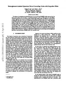
fore we have decreasing degrees of freedom to design the code words. 2.2 Support vector machines Support Vector Machines (SVM) recently gained popularity in the learning community [Vap98]. In its simplest linear form, an SVM is a hyperplane that separates a set of positive examples from a set of negative examples with maximum interclass distance, the margin. Figure 1 shows such a hyperplane with the associated margin. Figure 1 Hyperplane with maximal margin generated by a linear SVM Class 1 (w . x) + b > 0

Class 2

◆

(w . x) + b < 0 ●

●

()

31 = 2

1

Table 2 Minimal inter-row and inter-column Hamming distances for our codes. # code words 8 10 12 16 24 1-of-n

min. distance btw. class codes code words 2 14 3 16 4 14 6 14 10 14 1 1

See table 2.1 for the Hamming distances of a set of codes we used. In a code matrix of size l , i.e. a matrix with l code words, there are always class codes plus the -code. For larger numbers of code words, i.e. increasing l, the hamming distances grow. The reason is that the number of class codes to be generated re) and therefore we have more mains constant ( degrees of freedom to place the bits in the class codes. The Hamming distances of code words decrease with increasing l. Here, we have constant length of code ), but increasing numbers of them. Therewords (

2

2 31

0

= 32

= 32

◆ ◆ ◆

w ● ● ●

(w . x) + b = 0

hyperplane

The formula for the output of a linear SVM is u

=
+ w

x

(1)

b

where w is the normal vector to the hyperplane, and x is the input vector. The margin is defined by the distance of the hyperplane to the nearest of the positive and negative examples. Maximizing the margin can be expressed as an optimization problem: minimize

1k k 2 w

2

subject to yi

(
i + )  1 8i w

x

b

;

(2)

11

where xi is the i-th training example and yi 2 f? ; g is the correct output of the SVM for the i-th training example. Note that the hyperplane is only determined by the training instances xi on the margin, the support vectors. Of course, not all problems are linearly separable. Cortes and Vapnik [CV95] proposed a modification to the optimization formulation that allows, but penalizes, examples that fall on the wrong side of the decision boundary. The SVM can be extended to nonlinear models by mapping the input space into a very high-dimensional feature space chosen a priori. In this space the optimal separating hyperplane is constructed [BGV92] [Vap98, p.421].

The distinctive advantage of the SVM for text categorization is its ability to process many thousand different inputs. This opens the opportunity to use all words in a text directly as features. For each word wi the number of times of occurrence is recorded. Joachims [Joa98] used the SVM for the classification of text into different topic categories. Dumais et al. [DPHS98] use linear SVM for text categorization because they are both accurate and fast. They are 35 times faster to train than the next most accurate (a decision tree) of the tested classifiers. They apply SVM to the Reuters21578 collection, e-mails and web pages. Drucker at al. [DWV99] classify e-mails as spam and non spam. They find that boosting trees and SVM have similar performance in terms of accuracy and speed, but SVM train significantly faster.

Table 3 Table of tested combinations of frequency transformations and SVM kernels # 1 2 3 4 5 6 7 8 9 10 11 12 13 14 15 16 17 18 19 20 21 22 23 24 25 26 27 28 29 30 31 32 33 34 35 36 37 38 39 40

abbreviation relFreq0 relFreq1-d 2 relFreq1-d 3 relFreq2-g 1 relFreqImp0 relFreqImp1-d 2 relFreqImp1-d 3 relFreqImp2-g 1 relFreqL20 relFreqL21-d 2 relFreqL21-d 3 relFreqL22-g 1 relFreqL2Imp0 relFreqL2Imp1-d 2 relFreqL2Imp1-d 3 relFreqL2Imp2-g 1 logRelFreq0 logRelFreq1-d 2 logRelFreq1-d 3 logRelFreq2-g 1 logRelFreqImp0 logRelFreqImp1-d 2 logRelFreqImp1-d 3 logRelFreqImp2-g 1 logRelFreqL20 logRelFreqL21-d 2 logRelFreqL21-d 3 logRelFreqL22-g 1 logRelFreqL2Imp0 logRelFreqL2Imp1-d 2 logRelFreqL2Imp1-d 3 logRelFreqL2Imp2-g 1 tfidf0 tfidf1-d 2 tfidf1-d 3 tfidf2-g 1 tfidfL20 tfidfL21-d 2 tfidfL21-d 3 tfidfL22-g 1

coding; kernel rf & L1 ; linear rf & L1 ; quadr. poly. rf & L1 ; cubic poly. rf & L1 ; rbf rf & L1 & imp; linear rf & L1 & imp; quadr. poly. rf & L1 & imp; cubic poly. rf & L1 & imp; rbf rf & L2 ; linear rf & L2 ; quadr. poly. rf & L2 ; cubic poly. rf & L2 ; rbf rf & L2 & imp; linear rf & L2 & imp; quadr. poly. rf & L2 & imp; cubic poly. rf & L2 & imp; rbf log rf & L1 ; linear log rf & L1 ; quadr. poly. log rf & L1 ; cubic poly. log rf & L1 ; rbf log rf & L1 & imp; linear log rf & L1 & imp; quadr. poly. log rf & L1 & imp; cubic poly. log rf & L1 & imp; rbf log rf & L2 ; linear log rf & L2 ; quadr. poly. log rf & L2 ; cubic poly. log rf & L2 ; rbf log rf & L2 & imp; linear log rf & L2 & imp; quadr. poly. log rf & L2 & imp; cubic poly. log rf & L2 & imp; rbf tfidf & L1 ; linear tfidf & L1 ; quadr. poly. tfidf & L1 ; cubic poly. tfidf & L1 ; rbf tfidf & L2 ; linear tfidf & L2 ; quadr. poly. tfidf & L2 ; cubic poly. tfidf & L2 ; rbf

2.3 Transformations of frequency vectors As lexical units scale to different order of magnitude in larger documents, it is interesting to examine how term frequency information can be mapped to quantities which can efficiently be processed by SVM. For our empirical tests we use different transformations of type frequencies: relative frequencies and logarithmic frequencies. As the simplest “frequency-transformation” we use the term-frequencies f wk ; di themselves. The frequencies are multiplied by one of the importance weights described below and normalized to unit length. Relative frequencies f wk ; di with importance weight idf normalized with respect to L2 -norm have been used by Joachims [Joa98] and others. We also tested other combinations as for example relative frequencies with no importance weight normalized with respect to L1 -norm, which is defined by

(

)

(

rel1 (wk ; di )

F

=

)

f (wk ;di ) f (di )

The second transformation is the logarithm. We consider this transform because it is a common approach in quantitative linguistics to consider logarithms of linguistic quantities rather than the quantities themselves. Here we also normalize to unit length with respect to L1 and
L2 . We define Flog wk ; di ? f w k ; di , combine Flog different importance weights, and normalize the resulting vector with respect to L1 and L2 .

log 1+ (

)

(

) =

2.4 Importance weights Importance weights are often used in order to reduce dimensionality of a learning task. Common importance weights like inverse document frequency (idf) originally have been designed for identifying index words. However, since SVM are capable to manage a large number of dimensions ([KL00] used more than input features), reduction of dimensionality is not necessary and importance weights can be used to quantify how a specific given type is to the documents of a text collection. A type which is evenly distributed across the document collection will be given a low importance weight because it is judged to be less specific for the documents it occurs in, than a type which is used in a only a few documents. The importance weight of a type is multiplied by its transformed frequency of occurrence. So each of the importance weights described below can be combined with each of the frequency transformations described in section (2.3). We examined the performance of the following settings no importance weight, inverse document frequency (idf), and redundancy. Inverse document frequency (idf) is commonly used when SVM is

400000

log

n applied to text classification. Idf is defined by dfk , where dfk is the number of those documents in the collection, which contain the term wk and n is the number of all documents in the collection. Redundancy quantifies the skewness of a probability distribution. We consider the empirical distribution of each type over the different documents and define an importance weight by R

log + n

(

n X i=1

= max ? = ( k i ) log ( k i ) ( k) ( k) H

f w ;d

f w

f w

It is well known that the choice of the kernel function is crucial to the efficiency of support vector machines. Therefore the data transformations described above were combined with three different kernel functions: linear 2nd ord. poly. 3rd ord. poly. Gaussian

( ( ( (

0) 0 ~ x; ~ x ) 0 ~ x; ~ x ) 0 ~ x; ~ x )

K ~ x; ~ x K K K

=
0 = (
00) = (
) 2 = ?k~x?~x k=  ~ x

~ x

~ x

~ x

~ x

~ x

e

2

log;L1

log(1 + ( = P k (1 + (

0

2

In the following list we show the frequency transformations which were used.

log;red;L1

F

F

=

=

log(1 + ( k i )) ( k )  k log(1 + ( k i )) ( k )

rel;red;L1

(

k i) k i)

k

(

F

P

(9)–(12) relative frequency normalized with respect to L2 .

rel;L2

F

=

R w

F w ;d

R w

log;L2

=

log(1 + ( k i )) ?
 log 1 + ( ) k i k

(

k i) k F (wk ; di )2

F w ;d

pP

F w ;d

r P 

2

F w ;d

F

log(1 + ( k i)) ( k )  (1 + ( )) ( ) k i k k

=

log;L1

F w ;d

r P 

R w

2

F w ;d

R w

(33)–(36) tfidf normalized with respect to L1 F

k i ) log dfnk n k F (wk ; di ) log dfk

=

idf;L1

(

F w ;d

P

(37)–(40) tfidf normalized with respect to L2

idf;L2

F

=

(

k i ) log dfnk

F w ;d

r

P 

k

(

k i ) log dfnk

2

F w ;d

F w ;d

rel;red (wk ; di )R(wk ) k Frel;red (wk ; di )R(wk )

=

F w ;d

P 

F w ;d

P

(5)–(8) relative frequency with redundancy normalized with respect to L1 F

k i )) k i ))

F w ;d

(39)–(32) logarithmic frequencies with redundancy normalized with respect to L2

(1)–(4) relative frequency normalized with respect to

rel;L1

R w

F w ;d

40

F

k

2

i) ( k)

(21)–(24)logarithmic frequencies with redundancy normalized with respect to L1 .

3

In our experiments we tested combinations of kernel functions, frequency-transformations, importanceweights, and text-length-normalization. Table 3 summarizes the combinations of kernels. Its numbering and abbreviations are used throughout the rest of the paper.

L1

(

F w ;d

(25)–(28) logarithmic frequencies normalized with respect to L2 .

2.5 Kernel functions

   

k i )R(wk )

P 

(17)–(20) logarithmic frequencies normalized with respect to L1 .

(4)

)

(

F w ;d

r

k

F

where f wk ; di is the frequency of occurrence of term wk in document di and n is the number of documents in the collection. R is a measure of how much the distribution of a term wk in the various documents deviates from the uniform distribution.

=

rel;red;L2

F

(3)

H

f w ;d

(13)–(16) relative frequency with redundancy normalized with respect to L2

3 The experiments 3.1 The corpus We

use

the

Reuters-21578

dataset

http://www.research.att.com/˜lewis/reuters21578.html

compiled by David Lewis and originally collected by the Carnegie group from the Reuters newswire in 1987. We selected texts from the reuters collection along the following criteria: (i) The text length is 50 or more

running words. (ii) The text category is indicated and there is exactly one category. In total, we selected 6242 Texts which were categorized into 64 different topics. We furthermore selected 31 most frequent topics, summing up to 6024 texts. The remaining 218 texts were categorized as “NN”, regardless of their true category (which of course was different from our 31 selected categories). The names of the categories and number of texts in each category is displayed in table 4. Frequent categories such as “corn”, or “wheat” do not show up in our data set because they only appear in multi-category texts, which were excluded. To exploit the training set S0 of 6242 texts in a better way, we used the following cross-testing procedure. S0 was randomly divided into 3 subsets S1 ; : : : ; S3 of nearly equal size. Then five different SVM were determined using S0 n Si as training set of size  and Si was used as test set of size  . The numbers of correctly and wrongly classified documents were added up yielding an effective test set of all 6242 documents.

4161

2081

Table 4 Names of text categories and numbers of texts for each category. category earn acq crude trade money-fx interest ship sugar coffee gold mon.-supp.

data 1820 1807 349 330 230 164 151 127 107 97 91

category gnp cpi cocoa iron-steel grain jobs alum nat-gas reserves copper ipi

data 72 65 52 45 43 42 41 41 40 39 39

category rubber veg-oil tin cotton bop gas wpi livestock pet-chem NN

data 38 37 28 23 22 22 22 20 20 218

3.2 Definition of loss functions We consider the task to decide if a text previously unknown belongs to a given category or not. The specific setup is reflected in the loss function L i , which specifies the loss that incurs for the classification of o test set where i is the true class. The loss for the misclassification of a text was set to 1. We cannot decide apriori whether it is worse to categorize a wrong text to the topic in question than not to recognize a text which actually is in the category.

()

()

()

Let ctar i and etar i respectively denote the number of correctly and incorrectly classified documents of the target category i and let eoth i and let coth i be the same figures for the other categories in the alterna-

()

()

tive class. ptar is the prior probability that an unknown text belongs to a given class. Hence the loss for a the classification of a test set is

() tar ( ) + tar ( ) +(1 ? tar ) oth ( )oth+( )oth ( ) ( )=

L i

p

etar i

tar e

p

i

e

c

e

i

i

c

(5)

i

(6)

i

We assume that new texts to be classified arrive at the same ratio as in our corpus, i.e. ptar is computed as the fraction of texts in our corpus which belong to a given class. The mean number of texts in the 31 , and there are 6242 texts, i.e. the mean classes is  prior probability would be ptar =  : . But the fractions of texts in the 31 classes range from ptar : for the largest class to ptar : for the smallest class. Therefore we compute the losses for two different groups of classes. The first group includes the four large classes “earn”, “acq”, “crude”, and “trade” with more than of all texts. The mean prior is ptar : . The second group includes all other classes with mean ptar : . To allow comparisons we always report the loss for 1000 new classifications.

194

= 194 6242 0 031 = 0 0033

= 0 302

5% = 0 01

= 0 17

()

In addition we used the precision pprc i and the recall prec i to describe the result of an experiment.

()

( ) = tar ( )tar+( )oth( ) prc ( ) = 0 if tar ( ) = 0 c

pprc i p

c

i

i

i

e

c

i

(7)

;

(8)

i

( ) = ( )tar+( ) ( ) tar tar

prec i

c

c

i

i

e

(9)

i

Precision is the probability that a document predicted to be in a class truly belongs to this class. Recall is the probability that a document having a certain topic is classified into this class. A tradeoff exists between large recall and large precision.

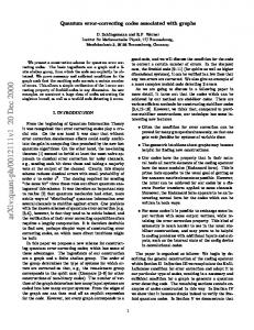
4 Results 4.1 Performance of frequency codings and kernels As already stated in ([KL00]), which examined the performance of SVM on Reuters and two German newspaper corpora, there are only small differences in performance for different SVM kernels. Figures 2 and 3 show the mean performances for -bit and -bit multi-class codes as compared to the -of-ncoding. Each of the frequency-kernel combinations

24

10

40

1

listed in section 2.5 is displayed. Figure 2 shows the mean performance of all classes in group 1 (see section 3.2). Figure 2 shows the mean performance of group 2 classes.

best. In figures 2 and 3 these combinations are marked by arrows. Figure 3 Mean loss of classes of group 2.

code length 10 code length 24 1−of−n−coding

frequency coding

frequency coding

relFreq0 relFreq1−d 2 relFreq1−d 3 relFreq2−g 1 relFreqImp0 relFreqImp1−d 2 relFreqImp1−d 3 relFreqImp2−g 1 relFreqL20 relFreqL21−d 2 relFreqL21−d 3 relFreqL22−g 1 relFreqL2Imp0 relFreqL2Imp1−d 2 relFreqL2Imp1−d 3 relFreqL2Imp2−g 1 logRelFreq0 logRelFreq1−d 2 logRelFreq1−d 3 logRelFreq2−g 1 logRelFreqImp0 logRelFreqImp1−d 2 logRelFreqImp1−d 3 logRelFreqImp2−g 1 logRelFreqL20 logRelFreqL21−d 2 logRelFreqL21−d 3 logRelFreqL22−g 1 logRelFreqL2Imp0 logRelFreqL2Imp1−d 2 logRelFreqL2Imp1−d 3 logRelFreqL2Imp2−g 1 tfidf0 tfidf1−d 2 tfidf1−d 3 tfidf2−g 1 tfidfL20 tfidfL21−d 2 tfidfL21−d 3 tfidfL22−g 1

code length 10

code length 24 1−of−n−coding

Figure 2 Mean loss of classes of group 1 for all frequency codings.

relFreq0 relFreq1−d 2 relFreq1−d 3 relFreq2−g 1 relFreqImp0 relFreqImp1−d 2 relFreqImp1−d 3 relFreqImp2−g 1 relFreqL20 relFreqL21−d 2 relFreqL21−d 3 relFreqL22−g 1 relFreqL2Imp0 relFreqL2Imp1−d 2 relFreqL2Imp1−d 3 relFreqL2Imp2−g 1 logRelFreq0 logRelFreq1−d 2 logRelFreq1−d 3 logRelFreq2−g 1 logRelFreqImp0 logRelFreqImp1−d 2 logRelFreqImp1−d 3 logRelFreqImp2−g 1 logRelFreqL20 logRelFreqL21−d 2 logRelFreqL21−d 3 logRelFreqL22−g 1 logRelFreqL2Imp0 logRelFreqL2Imp1−d 2 logRelFreqL2Imp1−d 3 logRelFreqL2Imp2−g 1 tfidf0 tfidf1−d 2 tfidf1−d 3 tfidf2−g 1 tfidfL20 tfidfL21−d 2 tfidfL21−d 3 tfidfL22−g 1

0

2

4

6

8

loss 0

5

10

15

20

25

30

loss

4.2 Small classes Importance weights improve the performance significantly. Redundancy defined in equation (3) is a better importance weight than the common inverse document frequency. We see that the transformations (logarithmic) relative frequency with redundancy normalized with respect to L2 combined with the linear kerand ) perform nel (i.e. combinations number

12

28

Table 5 shows the mean performance over all frequency codes and SVM kernels in terms of the loss function defined in equation 5. This time we show results for the -bit, -bit, and -bit multi-class codings. The classes of group 1 with ptar : are sep: . The arated from those of group 2 with ptar percentages of classes with better loss for the multi-

10

16

24

= 0 17 = 0 01

1

But if we combine several small classes so that the union has to be recognized, the overall fraction of the training set becomes larger, thus avoiding the adverse effects of very small classes. Another possibility to avoid over-fitting on small classes would be to change the cost function of the SVM training algorithm. We are also planning to investigate this option.

class codes than for the -of-n code is indicated below both groups in the table.

1

For group 1 (i.e. large) classes, -of-n coding and multi-class codings perform equally well. But for small classes, with less than of texts, the picture changes. Here, the loss of -bit and -bit multi-class codes is in many cases smaller than that of -of-n coding.

5%

24

1

Table 5 mean loss over all frequency codings for each code length and each category

230 164 151 127 107 97 91 72 65 52 45 43 42 41 41 40 39 39 38 37 28 23 22 22 22 20 20

loss of class code length : : : 10 16 24 1-of-n 22.18 23.91 20.769 16.32 35.21 39.37 35.182 23.30 20.60 17.33 15.296 28.94 23.60 17.80 16.536 34.19 50.0 12.73 13.43 10.11 4.56 3.10 5.41 4.49 6.28 3.68 1.76 6.00 9.69 3.72 5.16 6.35 5.35 3.89 5.42 5.89 8.50 2.22 4.26 10.68 13.93 10.18 7.12 11.20

50.0 9.18 6.05 6.07 2.18 1.41 1.52 3.22 6.04 3.87 3.48 3.74 6.71 2.41 4.16 3.90 3.39 3.92 4.08 2.60 4.58 1.70 3.24 6.75 4.40 3.78 7.04 9.25

50.0 11.978 6.667 3.439 1.242 1.056 1.849 2.644 3.826 2.353 0.923 3.652 4.455 1.479 3.085 3.597 2.577 2.376 3.436 1.425 3.973 0.933 2.833 6.170 5.008 3.811 5.298 9.149

– 7.26 5.33 4.26 1.33 1.08 2.48 2.66 4.48 3.09 2.32 5.94 6.89 2.89 6.86 5.90 4.15 4.19 5.37 4.01 5.15 5.05 4.82 7.27 5.64 4.92 6.58 9.68

18.5

63.0

92.6

–

An explanation for the better results of multi-class codes for small classes can be seen the over-fitting tendency of the learning algorithm. Classifiers like SVM tend to ignore a few cases of class “1”, when everything else is class “0”. Figures 4 and 5 support the claim: -of-n coding is especially strong at precision (eqn 7) on the cost of relatively weak recall (eqn 9).

1

1−of−n−coding

earn acq crude trade % better than 1-of-n money-fx interest ship sugar coffee gold money-supply gnp cpi cocoa iron-steel grain jobs alum nat-gas reserves copper ipi rubber veg-oil tin cotton bop gas wpi livestock pet-chem % better than 1-of-n

num. texts 1820 1807 349 330

relFreq0 relFreq1−d 2 relFreq1−d 3 relFreq2−g 1 relFreqImp0 relFreqImp1−d 2 relFreqImp1−d 3 relFreqImp2−g 1 relFreqL20 relFreqL21−d 2 relFreqL21−d 3 relFreqL22−g 1 relFreqL2Imp0 relFreqL2Imp1−d 2 relFreqL2Imp1−d 3 relFreqL2Imp2−g 1 logRelFreq0 logRelFreq1−d 2 logRelFreq1−d 3 logRelFreq2−g 1 logRelFreqImp0 logRelFreqImp1−d 2 logRelFreqImp1−d 3 logRelFreqImp2−g 1 logRelFreqL20 logRelFreqL21−d 2 logRelFreqL21−d 3 logRelFreqL22−g 1 logRelFreqL2Imp0 logRelFreqL2Imp1−d 2 logRelFreqL2Imp1−d 3 logRelFreqL2Imp2−g 1 tfidf0 tfidf1−d 2 tfidf1−d 3 tfidf2−g 1 tfidfL20 tfidfL21−d 2 tfidfL21−d 3 tfidfL22−g 1

frequency coding

category

Figure 4 Mean recall of classes of group 2.

code length 10 code length 24

16

0

20

40

60 recall

80

100

5 Conclusion

code length 10

1

50% 75%

We also will investigate a categorization task with a ), because a much larger number of classes (  larger number of classes implies that most of them will be small.

200

relFreq0 relFreq1−d 2 relFreq1−d 3 relFreq2−g 1 relFreqImp0 relFreqImp1−d 2 relFreqImp1−d 3 relFreqImp2−g 1 relFreqL20 relFreqL21−d 2 relFreqL21−d 3 relFreqL22−g 1 relFreqL2Imp0 relFreqL2Imp1−d 2 relFreqL2Imp1−d 3 relFreqL2Imp2−g 1 logRelFreq0 logRelFreq1−d 2 logRelFreq1−d 3 logRelFreq2−g 1 logRelFreqImp0 logRelFreqImp1−d 2 logRelFreqImp1−d 3 logRelFreqImp2−g 1 logRelFreqL20 logRelFreqL21−d 2 logRelFreqL21−d 3 logRelFreqL22−g 1 logRelFreqL2Imp0 logRelFreqL2Imp1−d 2 logRelFreqL2Imp1−d 3 logRelFreqL2Imp2−g 1 tfidf0 tfidf1−d 2 tfidf1−d 3 tfidf2−g 1 tfidfL20 tfidfL21−d 2 tfidfL21−d 3 tfidfL22−g 1

frequency coding

In our further work we will investigate the influence of different multi-class codes of the same length on error rates and test different optimization schemata for code generation. One option here is to introduce optimization weights into the code generation algorithm, which depend on statistical class properties. This could yield codes which help to classify small as well as large classes with the same accuracy.

References [BGV92] B.E.Boser, I.M. Guyon, and V.N. Vapnik. A training algorithm for optimal margin classifiers. In D.Haussler, editor, Proc. 5th ACM Workshop on Computational Learning Theory, pages 144– 152. ACM Press, 1992. [CV95] C. Cortes and V. Vapnik. Support vector networks. Machine Learning, 20:273–297, 1995. [DB95] T.G. Dietterich and G. Bakiri. Solving multiclass learning via error-correcting output codes. Journal of Artificial Intelligence Research, 2:263–286, 1995. [DPHS98] S. Dumais, J. Platt, D. Heckerman, and M. Sahami. Inductive learning algorithms and representations for text categorization. In 7th International Conference on Information and Knowledge Managment, 1998. [DWV99] H. Drucker, D. Wu, and V. Vapnik. Support vector machines for spam categorization. IEEE Transactions on Neural Networks, 10(5):1048– 1054, 1999. [GEPM00] Y. Guermeur, A. Eliseeff, and H. PaugamMoisy. A new multi-class svm based on a uniform convergence result. In S.-I. Amari, C.L. Giles, M. Gori, and V. Piuri, editors, Proceedings of the IEEE-INNS-ENNS International Joint Conference on Neural Networks IJCNN 2000, pages IV–183 – IV–188, Los Alamitos, 2000. IEEE Computer Society. [Joa98] T. Joachims. Text categorization with support vector machines: Learning with many relevant features. In C. Nedellec and C. Rouveirol, edi-

1−of−n−coding

We performed experiments for text categorization on a subset of the Reuters corpus. We investigated the influences of multi-class error correcting codes on the performance over a wide variety of frequency code and SVM kernel combinations. The main result is that multi-class codes have advantages over -of-n coding for classes which comprise only a small percentage of the data. Advantages were seen most clearly in the ::: size of the number range of codes with of classes to distinguish.

code length 24

Figure 5 Mean precision of classes of group 2.

0

20

40

60

80

100

precision

[KL00]

[NPP00]

tors, European Conference on Machine Learning (ECML), 1998. J. Kindermann and E. Leopold. Classification of texts with support vector machines. An examination of the efficiency of kernels and datatransformations. Paper accepted at 24th Annual Conference of the Gesellschaft f¨ur Klassifikation; 15 - 17 March, 2000 in Passau., 2000. C. Nakajima, M. Pontil, and T. Poggio. People recognition and pose estimation in image sequences. In S.-I. Amari, C.L. Giles, M. Gori, and V. Piuri, editors, Proceedings of the IEEE-INNSENNS International Joint Conference on Neural

[Vap98]

Networks IJCNN 2000, pages IV–189 – IV–196, Los Alamitos, 2000. IEEE Computer Society. V. N. Vapnik. Statistical Learning Theory. Wiley, New York, 1998.