Multi-Cloud Deployment of Computing Clusters for ... - Semantic Scholar

DRAFT FOR IEEE TPDS (SPECIAL ISSUE ON MANY-TASK COMPUTING), JULY 2010

1

Multi-Cloud Deployment of Computing Clusters for Loosely-Coupled MTC Applications Rafael Moreno-Vozmediano, Ruben S. Montero, Ignacio M. Llorente Abstract—Cloud computing is gaining acceptance in many IT organizations, as an elastic, flexible and variable-cost way to deploy their service platforms using outsourced resources. Unlike traditional utilities where a single provider scheme is a common practice, the ubiquitous access to cloud resources easily enables the simultaneous use of different clouds. In this paper we explore this scenario to deploy a computing cluster on top of a multi-cloud infrastructure, for solving loosely-coupled Many-Task Computing (MTC) applications. In this way, the cluster nodes can be provisioned with resources from different clouds to improve the cost-effectiveness of the deployment, or to implement high-availability strategies. We prove the viability of this kind of solutions by evaluating the scalability, performance, and cost of different configurations of a Sun Grid Engine cluster, deployed on a multi-cloud infrastructure spanning a local data-center and three different cloud sites: Amazon EC2 Europe, Amazon EC2 USA, and ElasticHosts. Although the testbed deployed in this work is limited to a reduced number of computing resources (due to hardware and budget limitations), we have complemented our analysis with a simulated infrastructure model, which includes a larger number of resources, and runs larger problem sizes. Data obtained by simulation show that performance and cost results can be extrapolated to large scale problems and cluster infrastructures.

Index Terms—Cloud computing, computing cluster, multi-cloud infrastructure, loosely-couple applications.

✦

1

I NTRODUCTION

M

A ny-Task Computing (MTC) paradigm [1] embraces different types of high-performance applications involving many different tasks, and requiring large number of computational resources over short periods of time. These tasks can be of very different nature, with sizes from small to large, loosely coupled or tightly coupled, or compute-intensive or data-intensive. Cloud computing technologies can offer important benefits for IT organizations and data-centers running MTC applications: elasticity and rapid provisioning, enabling the organization to increase or decrease its infrastructure capacity within minutes, according to the computing necessities; pay-as-you-go model, allowing organizations to purchase and pay for the exact amount of infrastructure they require at any specific time; reduced capital costs, since organizations can reduce or even eliminate their in-house infrastructures, resulting on a reduction in capital investment and personnel costs; access to potentially “unlimited” resources, as most cloud providers allow to deploy hundreds or even thousands of server instances simultaneously; and flexibility, because the user can deploy cloud instances with different hardware configurations, operating systems, and software packages. Computing clusters have been one of the most popular platforms for solving MTC problems, specially in the case of loosely coupled tasks (e.g. high-throughput com• R. Moreno-Vozmediano, R. S. Montero and I.M. Llorente are with the Dept. of Computer Architecture, Complutense University of Madrid, Spain. E-mail: {rmoreno, rubensm, llorente}@dacya.ucm.es Manuscript received December xx, 2009; revised xx xx, 2010.

puting applications). However, building and managing physical clusters exhibits several drawbacks: 1) major investments in hardware, specialized installations (cooling, power, etc.), and qualified personal; 2) long periods of cluster under-utilization; 3) cluster overloading and insufficient computational resources during peak demand periods. Regarding these limitations, cloud computing technology has been proposed as a viable solution to deploy elastic computing clusters, or to complement the in-house data-center infrastructure to satisfy peak workloads. For example, the BioTeam [2] has deployed the Univa UD UniCluster Express in an hybrid setup, which combines local physical nodes with virtual nodes deployed in the Amazon EC2. In a recent work [3], we extend this hybrid solution by including virtualization in the local site, so providing a flexible and agile management of the whole infrastructure, that may include resources from remote providers. However, all these cluster proposals are deployed using a single cloud, while multi-cloud cluster deployments are yet to be studied. The simultaneous use of different cloud providers to deploy a computing cluster spanning different clouds can provide several benefits: •

•

High-availability and fault tolerance, the cluster worker nodes can be spread on different cloud sites, so in case of cloud downtime or failure, the cluster operation will not be disrupted. Furthermore, in this situation, we can dynamically deploy new cluster nodes in a different cloud to avoid the degradation of the cluster performance. Infrastructure cost reduction, since different cloud providers can follow different pricing strategies, and


even variable pricing models (based on the level of demand of a particular resource type, daytime versus night-time, weekdays versus weekends, spot prices, and so forth), the different cluster nodes can change dynamically their locations, from one cloud provider to another one, in order to reduce the overall infrastructure cost. The main goal of this work is to analyze the viability, from the point of view of scalability, performance, and cost of deploying large virtual cluster infrastructures distributed over different cloud providers for solving loosely coupled MTC applications. This work is conducted in a real experimental testbed that comprises resources from our in-house infrastructure, and external resources from three different cloud sites: Amazon EC2 (Europe and USA zones1 ) [4] and ElasticHosts [5]. On top of this distributed cloud infrastructure, we have implemented a Sun Grid Engine (SGE) cluster, consisting of a front-end and a variable number of worker nodes, which can be deployed on different sites (either locally or in different remote clouds). We analyze the performance of different cluster configurations, using the cluster throughput (i.e. completed jobs per second) as performance metric, proving that multi-cloud cluster implementations do not incur in performance slowdowns, compared to single-site implementations, and showing that the cluster performance (i.e. throughput) scales linearly when the local cluster infrastructure is complemented with external cloud nodes. In addition, we quantify the cost of these cluster configurations, measured as the cost of the infrastructure per time unit, and we also analyze the performance/cost ratio, showing that some cloud-based configurations exhibit similar performance/cost ratio than local clusters. Due to hardware limitations of our local infrastructure, and the high cost of renting many cloud resources for long periods, the tested cluster configurations are limited to a reduced number of computing resources (up to 16 worker nodes), running a reduced number of tasks (up to 128 tasks). However, as typical MTC applications can involve much more tasks, we have implemented a simulated infrastructure model, that includes a larger number of computing resources (up to 256 worker nodes), and runs a larger number of tasks (up to 5,000). The simulation of different cluster configurations shows that performance and cost results can be extrapolated to large scale problems and cluster infrastructures. More specifically, the contributions of this work are the following: 1) Deployment of a multi-cloud virtual infrastructure spanning four different sites: our local data-center, Amazon EC2 Europe, Amazon EC2 USA, and ElasticHosts; and implementation of a real computing cluster testbed on top of this multi-cloud infrastructure. 1. Amazon EC2 regions available in October 2009.

2

2) Performance analysis of the cluster testbed for solving loosely-coupled MTC applications (in particular, an embarrassingly parallel problem), proving the scalability of the multi-cloud solution for this kind of workloads. 3) Cost and cost-performance ratio analysis of the experimental setup, to compare the different cluster configurations, and proving the viability of the multi-cloud solution also from a cost perspective. 4) Implementation of a simulated infrastructure model to test larger sized clusters and workloads, proving that results obtained in the real testbed can be extrapolated to large scale multi-cloud infrastructures.

2 D EPLOYMENT C LUSTER

OF A

M ULTI -C LOUD V IRTUAL

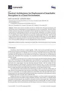
Fig. 1 shows the distributed cluster testbed used in this work deployed of top of a multi-cloud infrastructure. This kind of multi-cloud deployment involves several challenges, related to the lack of a cloud interface standard; the distribution and management of the service master images; and the interconnection links between the service components. A brief discussion of these issues, and the main design decisions adopted in this work to face up these challenges are included in the Appendix A of the supplemental material.

Fig. 1. Experimental framework Our experimental testbed starts from a virtual cluster deployed in our local data center, with a queuing system managed by Sun Grid Engine (SGE) software, and consisting of a cluster front-end (SGE master) and a fixed number of virtual worker nodes (four nodes in this setup). This cluster can be scaled-out by deploying new virtual worker nodes on remote clouds. The cloud providers considered in this work are Amazon EC2 (Europe and USA zones) and ElasticHosts. Table 1 shows the main characteristics of in-house nodes and cloud nodes used in our experimental testbed.


Besides the hardware characteristics of different testbed nodes, Table 1 also displays the cost per time unit of these resources. In the case of cloud resources, this cost represents the hourly cost charged by the cloud provider for the use of its resources2 . Appendix B.1 of supplemental material gives more details about the cost model used for cloud resources. On the other hand, the cost of the local resources is an estimation based on the model proposed by Walker [6] that takes into account the cost of the computer hardware, the cooling and power expenses, and support personnel. For more information about the application of this cost model to our local data center, see Appendix B.2. TABLE 1 Characteristics of different cluster nodes Site

Arch.

Local data center (L) Amazon EC2 Europe (AE) Amazon EC2 USA (AU) ElasticHosts (EH)

i686 32bits i686 32bits i686 32bits AMD 64-bits

Processor (single core) Xeon 2.0GHz

Mem. (GB) 1.0

Cost (USD/hour) 0.04

Xeon 1.2GHz

1.7

0.11

Xeon 1.2GHz

1.7

0.10

Opteron 2.1GHz

1.0

0.12

2.1 Performance Analysis In this section we analyze and compare the performance offered by different configurations of the computing cluster, focused in the execution of loosely-coupled applications. In particular, we have chosen 9 different cluster configurations (with different number of worker nodes from the three cloud providers), and different number of jobs (depending on the cluster size), as shown in Table 2. In the definition of the different cluster configurations, we use the following acronyms: L: Local infrastructure; AE: Amazon EC2 Europe cloud; AU: Amazon EC2 USA cloud; EH: ElasticHosts cloud. The number preceding the site acronym represents the number of worker nodes. For example, 4L is a cluster with four worker nodes deployed in the local infrastructure; and 4L+4AE is a eightnode cluster, four deployed in the local infrastructure and four in the Amazon EC2 Europe To represent the execution profile of loosely-coupled applications, we will use the Embarrassingly Distributed (ED) benchmark from the Numerical Aerodynamic Simulation (NAS) Grid Benchmarks [7] (NGB) suite. The ED benchmark consists of multiple independent runs of a flow solver, each one with a different initialization constant for the flow field. NGB defines several problem sizes (in terms of mesh size, iterations, and number of jobs) as classes S, W, 2. Prices charged by cloud providers in October 2009.

3

TABLE 2 Cluster configurations Exp. ID. 1 2 3 4 5 6 7 8 9

Worker Nodes 4 4 4 4 8 8 8 12 16

Cluster configuration 4L 4AE 4AU 4EH 4L+4AE 4L+4AU 4L+4EH 4L+4AE+4AU 4L+4AE+4AU+4EH

No. jobs 32 32 32 32 64 64 64 128 128

A, B, C, D and E. We have chosen a problem size of class B, since it is appropriate (in terms of computing time) for middle-class resources used as cluster worker nodes. However, instead of submitting 18 jobs, as ED class B defines, we have submitted a higher number of jobs (depending on the cluster configuration, see Table 2) in order to saturate the cluster and obtain realistic throughput measures. As we have proven in a previous work [8], when executing loosely coupled high throughput computing applications, the cluster performance (in jobs completed per second) can be easily modeled using the following equation: r∞ (1) r(n) = 1 + n1/2 /n where n is the number of jobs completed, r∞ is the asymptotic performance (maximum rate of performance of the cluster in jobs executed per second), and n1/2 is the half-performance length. For more details about this performance model see Appendix C of the supplemental material. Fig. 2 shows the experimental cluster performance and that predicted by (1). As can be observed from these plots the performance model defined in equation (1) provides a good characterization of the clusters in the execution of the workload under study. Table 3 shows the r∞ and n1/2 parameters of the performance model for each cluster configuration. The parameter r∞ can be used as a measure of cluster throughput, in order to compare the different cluster configurations, since it is a accurate approximation for the maximum performance (in jobs per second) of the cluster in saturation. Please, note that we have achieved five runs of each experiment, so data in Table 3 represent the mean values of r∞ and n1/2 (standard deviations can be found in Appendix C). If we compare 4L and 4EH configurations, we observe that they exhibit very similar performance. This is because of two main reasons: first, worker nodes from both sites have similar CPU capacity (see Table 1); and second, communication latencies for this kind of loosely coupled applications do not cause significant performance degradation, since data transfer delays are negligible compared to execution times, mainly thanks


4

for the particular workload considered in this work, the use of a multi-cloud infrastructure spanning different cloud providers is totally viable from the point of view of performance and scalability, and does not introduce important overheads, which could cause significant performance degradation.

Fig. 3. Asymptotic performance (r∞ ) comparison

2.2 Cost Analysis Fig. 2. Throughput for different cluster configurations TABLE 3 Performance model parameters Exp. ID 1 2 3 4 5 6 7 8 9


r∞ 5.16 × 10−3 2.92 × 10−3 2.83 × 10−3 5.58 × 10−3 7.90 × 10−3 7.81 × 10−3 1.08 × 10−2 1.12 × 10−2 1.76 × 10−2

n1/2 1.7 1.6 1.6 2.4 3.9 3.9 5.0 5.4 7.6

to the NFS file data caching implemented on the NFS clients (worker nodes), which notably reduces the latency of NFS read operations. On the other hand, the lower performance of 4AE and 4AU configurations is mainly due to the lower CPU capacity of the Amazon EC2 worker nodes (see Table 1). An important observation is that cluster performance for hybrid configurations scales linearly. For example, if we observe the performance of 4L+4AE configuration, and we compare it with the performance of 4L and 4AE configurations separately, we find that the sum of performances of these two individual configurations is almost similar to the performance of 4L+4AE configuration. This observation is applicable to all of the hybrid configurations, as shown in Fig. 3. This fact proves that,

Besides the performance analysis, the cost of cloud resources also has important impact on the viability of the multi-cloud solution. From this point of view, it is important to analyze, not only the total cost of the infrastructure, but also the ratio between performance and cost, in order to find the most optimal configurations. The average cost of each instance per time unit is gathered in Table 1. Based on these costs, and using the cost model detailed in Appendix B of the supplemental material, we can estimate the cost of every experiment. However this cost is not suitable to compare the different cluster configurations, since we are running different number of jobs for every configuration. So, in order to normalize the cost of different configurations, we have computed the cost per job, shown in Fig. 4, by dividing the cost of each experiment by the number of jobs in the experiment. As the cost of local resources is lower than the cloud resources, it is obvious 4L configuration results in the experiment with the lowest cost per job. Similarly, those experiments including only cloud nodes (e.g. 4AE, 4AU, and 4EH) exhibit higher price per job than those hybrid configurations including local and cloud nodes (e.g. 4L+4AE, 4L+4AU, and 4L+4EH). We also observe that, for the particular workload used in this experiment, configurations including EH nodes result in a lower cost per job than those configurations including Amazon nodes (e.g. 4EH compared to 4AE and 4AU, or 4L+4EH compared to 4L+4AE and 4L+4AU). Regarding these comparative cost results, it is obvious that, for large organizations that make intensive use of computational resources, the investment on a rightsized local data center can be more cost-effective than leasing resources to external cloud providers. However,


Fig. 4. Cost per job for different configurations

5

conducted by the real results obtained with the experimental testbed, which includes a larger number of computing resources (up to 256 worker nodes in the simulated infrastructure), and runs a larger number of tasks (up to 5,000). The details and validation of the simulator used in this section can be found in the Appendix D of the supplemental material. In addition, Appendix E analyzes the NFS server performance for the cluster sizes used in our simulation experiments, and proves that, for loosely coupled workloads, the NFS server is not a significant bottleneck, and it has little influence on cluster performance degradation. We have simulated different cluster configurations (see Table 4), each one running 5,000 independent tasks belonging to the NGB ED class B benchmark. The throughput results of these simulations are displayed in Fig. 6. Table 4 summarizes the asymptotic performance (r∞ , expressed in jobs/s) obtained for each configuration.

Fig. 5. Performance/cost ratio for different configurations

for small companies or small research communities, the use of cloud-based computing infrastructures can be much more useful, from a practical point of view, than setting up their own computing infrastructure. Finally, to decide what configurations are optimal from the point of view of performance and cost, we have computed the ratio between cluster performance (r∞ ) and cost per job, as shown in Fig. 5 (we show the normalized values with respect to the 4L case). We can observe that, in spite of the higher cost of cloud resources with respect local nodes, there are some hybrid configurations (4L+4EH, and 4L+4AE+4AU+4EH) that exhibit better performance-cost ratio than the local setup (4L configuration). This fact proves that the proposed multi-cloud implementation of a computing cluster can be an interesting solution, not only from the performance point of view, but also from a cost perspective.

3

S IMULATION R ESULTS

The previous section shows a performance and cost analysis for different configurations of a real implementation of a multi-cloud cluster infrastructure running a real workload. However, due to hardware limitations in our local infrastructure, and the high cost of renting many cloud resources for long periods, the tested cluster configurations are limited to a reduced number of computing resources (up to 16 worker nodes in the cluster), running a reduced number of tasks (up to 128 tasks). However, as the goal of this paper is to show the viability of these multi-cloud cluster solutions for solving MTC problems, which can involve much more tasks, we have implemented a simulated infrastructure model,

Fig. 6. Throughput for simulated cluster configurations

TABLE 4 Simulation results for different cluster configurations Sim. ID 1 2 3 4 5 6 7 8 9


r∞ 0.083 0.046 0.045 0.089 0.128 0.128 0.171 0.172 0.259

Looking at throughput results, we can conclude that the experimental results obtained for the real testbed can be extrapolated to larger sized clusters and higher number of tasks. In fact, we observe in Table 4 that the asymptotic performance for the simulated model scales linearly when we add cloud nodes to the local cluster configuration. For example, we find that the asymptotic performance of 64L+64AE configuration is almost similar to sum of the performances of 64L and 64AE configurations separately. Similar observations can be made for the rest of cluster configurations. Regarding the cost analysis for simulated infrastructures, summarized in Fig. 7, we observe that cost


per job results for the real testbed can also be extrapolated to larger clusters, namely, hybrid configurations including local and cloud nodes (e.g. 64L+64AE, 64L+64AU, and 64L+64EH) exhibit lower cost per job than those configurations with only cloud nodes (e.g. 64AE, 64AU, and 64EH); and configurations including EH nodes result in a lower cost per job than configurations including Amazon nodes (e.g. 64EH compared to 64AE and 64AU, or 64L+64EH compared to 64L+64AE and 64L+64AU). Finally, analyzing the performance-cost ratio of the simulated infrastructures in Fig. 8, we see again a similar behavior to that observed for the real testbed, with some hybrid configurations (64L+64EH, and 64L+64AE+64AU+64EH) exhibiting better performance-cost ratio than the local setup (64L).

Fig. 7. Cost per job for simulated configurations

6

rapid, automated, on-the-fly partitioning of a physical cluster into multiple independent virtual clusters. Similarly, the VIOcluster [13] project enables to dynamically adjust the capacity of a computing cluster by sharing resources between peer domains. Several studies have explored the use of virtual machines to provide custom cluster environments. In this case, the clusters are usually completely build up of virtualized resources, as in the Globus Nimbus project [14], or the Virtual Organization Clusters (VOC) proposed in [15]. Some recent works [2], [3] have explored the use of cloud resources to deploy hybrid computing clusters, so the cluster combines physical, virtualized and cloud resources. There are many other different experiences on deploying different kind of multi-tier services on cloud infrastructures, such as web servers [16], database appliances [17], or web service platforms [18], among others. However, all these deployments only consider a single cloud, and they do not take advantage of the potential benefits of multi-cloud deployments. Regarding the use of multiple clouds, K. Keahey et al. introduce in [19] the concept of “Sky Computing”, which enables the dynamic provisioning of distributed domains over several clouds, and discusses the current shortcomings of this approach, such as image compatibility among providers, need of standards at API level, need of trusted networking environments, etc. This work also compares the performance of two virtual cluster deployed in two settings: a single-site deployment and a three-site deployment, and concludes that the performance of a single-site cluster can be sustained using a cluster across three sites. However, this work lacks a cost analysis and the performance analysis is limited to small size infrastructures (up to 15 computer instances, equivalent to 30 processor)

5

C ONCLUSIONS

AND

F UTURE WORK

Fig. 8. Perf.-cost ratio for simulated configurations

4

R ELATED WORK

Efficient management of large scale cluster infrastructures has been explored for years, and different techniques for on-demand provisioning, dynamic partitioning, or cluster virtualization have been proposed. Traditional methods for the on-demand provision of computational services consist in overlaying a custom software stack on top of an existing middleware layer. For example the MyCluster Project [9] creates a Condor or a SGE cluster on top of TeraGrid services. The Falkon system [10] provides a light high-throughput execution environment on top of the Globus GRAM service. Finally, the GridWay meta-scheduler [11] has been used to deploy BOINC networks on top of the EGEE middleware. The dynamic partitioning of the capacity of a computational cluster has also been addressed by several projects. For example the Cluster On Demand software [12] enables

In this paper we have analyzed the challenges and viability of deploying a computing cluster on top of a multi-cloud infrastructure spanning four different sites for solving loosely coupled MTC applications. We have implemented a real testbed cluster (based on a SGE queuing system) that comprises computing resources from our in-house infrastructure, and external resources from three different clouds: Amazon EC2 (Europe and USA zones) and ElasticHosts. Performance results prove that, for the MTC workload under consideration (loosely coupled parameter sweep applications), cluster throughput scales linearly when the cluster includes a growing number of nodes from cloud providers. This fact proves that the multi-cloud implementation of a computing cluster is viable from the point of view of scalability, and does not introduce important overheads, which could cause significant performance degradation. On the other hand, the cost analysis shows that, for the workload considered, some


hybrid configurations (including local and cloud nodes) exhibit better performance-cost ratio than the local setup, so proving that the multi-cloud solution is also appealing from a cost perspective. In addition, we have also implemented a model for simulating larger cluster infrastructures. The simulation of different cluster configurations shows that performance and cost results can be extrapolated to large scale problems and clusters. It is important to point out that, although the results obtained are very promising, they can differ greatly for other MTC applications with a different data pattern, synchronization requirement or computational profile. The different cluster configurations considered in this work have been selected manually, without considering any scheduling policy or optimization criteria, with the main goal of analyzing the viability of the multi-cloud solution from the points of view of performance and cost. Although a detailed analysis and comparison of different scheduling strategies is out of the scope of this paper, and it is planned for further research, for the sake of completeness, the Appendix F of the supplemental material presents some preliminary results on dynamic resource provisioning, in order to highlight the main benefits of multi-cloud deployments, such as infrastructure cost reduction, high-availability and fault tolerance capabilities.

ACKNOWLEDGMENTS This research was supported by Consejer´ıa de Educacion ´ of Comunidad de Madrid, Fondo Europeo de Desarrollo Regional, and Fondo Social Europeo through MEDIANET Research Program S2009/TIC-1468; by Ministerio de Ciencia e Innovacion ´ of Spain through research grant TIN2009-07146; and European Union through the research project RESERVOIR Grant Agreement 215605.

R EFERENCES [1] [2] [3] [4] [5] [6] [7] [8]

[9]

I. Raicu, I. Foster, Y. Zhao, Many-Task Computing for Grids and Supercomputers, Workshop on Many-Task Computing on Grids and Supercomputers, 2008, pp. 1–11 BioTeam, Howto: Unicluster and Amazon EC2, Tech. rep., BioTeam Lab Summary (2008). I. Llorente, R. Moreno-Vozmediano, R. Montero, Cloud Computing for On-Demand Grid Resource Provisioning, Advances in Parallel Computing, Vol. 18 (2009), IOS Press, pp. 177–191. Amazon Elastic Compute Cloud, http://aws.amazon.com/ec2. ElasticHosts, http://www.elastichosts.com/. E. Walker, The Real Cost of a CPU Hour. Computer 42(4): 35–41, 2009. M. A. Frumkin, R. F. Van der Wijngaart, NAS Grid Benchmarks: A Tool for Grid Space Exploration, J. Cluster Computing 5 (3): 247–255, 2002. R.S. Montero, R. Moreno-Vozmediano. I.M. Llorente, An Elasticity Model for High Throughput Computing Clusters. J. Parallel and Distributed Computing (in press, DOI: 10.1016/j.jpdc.2010.05.005), 2010. Walker, E., Gardner, J., Litvin, V., and Turner, E. Creating personal adaptive clusters for managing scientific jobs in a distributed computing environment. IEEE Challenges of Large Applications in Distributed Environments, 2006.

7

[10] Raicu, I., Zhao, Y., Dumitrescu, C., Foster, I., and Wilde, M. Falkon: a Fast and Light-weight tasK executiON farmework. IEEE/ACM SuperComputing, 2007. [11] Huedo, E., Montero, R. S., and Llorente, I. M. The GridWay Framework for Adaptive Scheduling and Execution on Grids. Scalable Computing – Practice and Experience, 6, 1–8, 2006. [12] Chase, J., Irwin, D., Grit, L., Moore, J., and Sprenkle, S. Dynamic Virtual Clusters in a Grid Site Manager. 12th IEEE Symp. on High Performance Distributed Computing, 2003. [13] Ruth, P., McGachey, P., and Xu, D. VioCluster: Virtualization for Dynamic Computational Domains. IEEE Int. Conference on Cluster Computing, 2005. [14] I. Foster, T. Freeman, K. Keahey, D. Scheftner, B. Sotomayor, and X. Zhang, Virtual clusters for grid communities, 6th IEEE Int. Symp. on Cluster Computing and the Grid, 2006. [15] M. Murphy, B. Kagey, M. Fenn, and S. Goasguen, Dynamic Provisioning of Virtual Organization Clusters, 9th IEEE Int. Symp. on Cluster Computing and the Grid, 2009. [16] J. Fronckowiak, Auto-scaling Web Sites using Amazon EC2 and Scalr, Amazon EC2 Articles and Tutorials, 2008. [17] A. Aboulnaga, K. Salem, A. Soror, U. Minhas, P. Kokosielis, S. Kamath, Deploying Database Appliances in the Cloud, Bulletin of the Technical Committee on Data Engineering, IEEE Computer Society 32 (1): 13–20, 2009. [18] A. Azeez, Autoscaling Axis2 Web Services on Amazon EC2,: ApacheCon Europe, 2009. [19] K. Keahey, M. Tsugawa, A. Matsunaga, and J. Fortes. Sky computing. IEEE Internet Computing, 13(5):43–51, 2009.

Rafael Moreno received the M.S. degree in Physics and the Ph.D. degree from the Universidad Complutense de Madrid (UCM), Spain, in 1991 and 1995 respectively. Since 1997 he is an Associate Professor of Computer Science and Electrical Engineering at the Department of Computer Architecture of the UCM, Spain. He has about 18 years of research experience in the fields of High-Performance Parallel and Distributed Computing, Grid Computing and Virtualization.

Ruben S. Montero , PhD is an associate professor in the Department of Computer Architecture at Complutense University of Madrid. Over the last years, he has published more than 70 scientific papers in the field of High-Performance Parallel and Distributed Computing, and contributed to more than 20 research and development programmes. His research interests lie mainly in resource provisioning models for distributed systems, in particular: Grid resource management and scheduling, distributed management of virtual machines and cloud computing.

Ignacio M. Llorente has a graduate degree in Physics (B.S. in Physics and M.S. in Computer Science), a Ph.D. in Physics (Program in Computer Science) and an Executive Master in Business Administration. He has about 17 years of research experience in the field of High Performance Parallel and Distributed Computing, Grid Computing and Virtualization. Currently, he is a Full Professor at Universidad Complutense de Madrid, where he leads the Distributed Systems Architecture Group.

SUPPLEMENTAL MATERIAL: MULTI-CLOUD DEPLOYMENT OF COMPUTING CLUSTERS FOR LOOSELY-COUPLED MTC APPLICATIONS.

1

Supplemental Material: Multi-Cloud Deployment of Computing Clusters for Loosely-Coupled MTC Applications. Rafael Moreno-Vozmediano, Ruben S. Montero, Ignacio M. Llorente

✦

A PPENDIX A C HALLENGES AND D ESIGN D ECISIONS ON M ULTI -C LOUD D EPLOYMENT OF V IRTUALIZED C LUSTERS The two cloud providers considered in this work are Amazon EC2 (Europe and USA regions), and ElasticHosts (EH). Although both cloud providers offer IaaS (Infrastructure as a Service) platforms and services, there are some technical differences between the EC2 and EH clouds: the EH infrastructure is based in KVM; all the storage provided is persistent; and there is no notion of instance type as users can customize the hardware setup of the VMs and define arbitrary capacity for them. Also, both providers use different price and billing schemes: EH adapts the price according to the configuration selected by the user; also EH uses hourly rates but offers discounts to users who sign for at least a month. There is no equivalent for the EC2 spot-price scheme in EH. The simultaneous use of different providers to deploy a virtualized service spanning different clouds involves several challenges, related to the lack of a cloud interface standard; the distribution and management of the service master images; and the interconnection links between the service components. In this section, we briefly analyze these issues and the main design decisions adopted in our experimental testbed to face up to them. Next, we briefly analyze some of the main challenges in multi-cloud deployments, regarding cloud interfacing, image management, and network management, and we present the main design decisions adopted in our experimental testbed to face up to these issues.

distributed– can also improve the cost-effectiveness, high availability or efficiency of the virtualized service. This challenges have been identified by the cloud community (see for example the Open Cloud Manifesto [1]) and several standardization efforts are working in different aspects of a Cloud, from formats, like the Open virtualization Format (OVF) from the distributed management task force (DMTF) [2], to cloud interfaces, for example the Open Cloud Computing Interface from the Open Grid Forum [3]. In this area, there are other initiatives that try to abstract the special features of current implementations by providing a common API to interface multiple clouds, see for example the Delta Cloud project [4] or libcloud [5]. However, there is no standard way to interface with a cloud, and each provider exposes its own APIs. Moreover the semantics of these interfaces are adapted to the particular services that each provider offers to its customer (e.g. firewall services, additional storage or specific binding to a custom IP). A traditional technique to achieve the inter-operation in this scenario, i.e. between middleware stacks with different interfaces, is the use of adapters [6]. In this context, an adapter is a software component that allows one system to connect to and work with a given cloud. In this work we will use the OpenNebula virtual infrastructure manager [7] as Cloud Broker. OpenNebula provides the functionality needed to deploy, monitor and control virtual machines (VM) on a pool of distributed physical resources, usually organized in a cluster-like architecture. In addition, OpenNebula also provide adapters to inter-operate with Amazon EC2 and ElasticHosts (EH) clouds (see Fig. 1).

A.1 Cloud Interfaces

A.2 Image Management

Cloud interoperability is probably one of aspects that is receiving more attention by the community. The need for interoperable clouds is two folded: first, the ability to easily move a virtualized infrastructure among different providers would prevent vendor locking; and secondly, the simultaneous use of multiple clouds –geographically

In general, a virtualized service consists in one or more components each one supported by one or more virtual machines. Instances of the same component are usually obtained by cloning a master image for that component, that contains a basic OS installation and the specific software required by the service.


Cloud providers use different formats and bundling methods to store and upload these master images. In this work we assume that suitable service component images (SGE worker nodes in our case) has been previously packed and registered in each cloud provider storage service. So when a VM is to be deployed in a given cloud the image adapters skip any image transfer operation. Note that this approach minimizes the service deployment time as no additional transfers are needed to instantiate a new service component. However there are some drawbacks associated to the storage of one master image in each cloud provider: higher service development cycles as images have to be prepared and debug for each cloud; higher costs as clouds usually charge for the storage used; and higher maintenance costs as new images have to be distributed to each cloud. A.3 Network Management Resources running on different cloud providers are located in different networks, and may use different addressing schemes (public addresses, private addresses with NAT, etc.). However, some kind of services require all their components to follow a uniform IP address scheme (for example, to be located on the same local network), so it could be necessary to build some kind of overlay network on top of the physical network to communicate the different service components. In this context, there are some interesting research proposals like ViNe [8], CLON [9], etc., or some commercial tools, like VPN-Cubed [10], which provide different overlay network solutions for grid and cloud computing environments. This network overlay provides the VMs with the same address space by placing specialized routers in each cloud –usually user-level virtual routers– that act as gateways for the VMs running in that cloud. Note that these solutions does not require to modify the cluster VMs. In this work we propose the use of Virtual Private Network (VPN) technology to interconnect the different cloud resources with the in-house data center infrastructure in a secure way. In particular, we use OpenVPN [11] software to implement Ethernet tunnels between each individual cloud resource and the data center LAN, as

Fig. 1. OpenNebula used as resource cloud broker

2

Fig. 2. VPN-based network configuration for a multi-cloud infrastructure shown in Fig. 2. In this setup, which follows a clientserver approach, the remote cloud resources, configured as VPN clients, establish an encrypted VPN tunnel with in-house VPN server, so that each client enables a new network interface which is directly connected to the data center LAN. In this way, resources located at different clouds can communicate among them, and with local resources, as they were located in the same logical network, and they can access to common LAN services (NFS, NIS, etc.) in a transparent way, as local resources do.

A PPENDIX B C OST E STIMATION M ODELS B.1 Cost Model for Cloud Resources The cost of leased resources from cloud providers are mainly derived from three sources: computing resources, storage, and network data transfer. These costs have been analyzed by different authors in the context of single-cloud based testbeds running high-performance computing applications. For example, Juve et al. [12] achieve an experimental study of the performance of three typical HPC workflows with different I/O, memory and CPU requirements on a commercial cloud (Amazon EC2, using different instance types), and compare the cloud performance to a typical HPC system (NCSAs Abe cluster). In addition, they also analyze the various costs associated with running these workflows using different EC2 instance types, namely, the resource cost, the storage cost, and the transfer cost. Regarding the results of this cost analysis, they conclude that the primary cost was in acquiring resources to execute workflow tasks, and that storage costs were relatively small in comparison. The cost of data transfers, although relatively high, can be effectively reduced by storing data in the cloud rather than transferring it for each workflow. In a previous work, Deelman et al. [13] also analyzes the costs of running a data-intensive application (Montage)


in Amazon EC2, and also conclude that the primary cost for this workload is due to computing resources. In our work, we analyze the deployment of a computing cluster in a multi-cloud environment, using resources from our local data center, and resource from three different cloud sites: Amazon EC2 Europe, Amazon EC USA, and ElasticHosts. These providers can offer different pricing schemes for computing resources, e.g. ondemand instances, reserved instances, or spot instances in Amazon EC2; and monthly subscription instances, or hourly burst instances in ElasticHosts. However, in this work we have used a single pricing method, based on a pay per compute capacity used scheme, which is available in most of cloud providers (on-demand instances in Amazon EC2, and hourly burst instances in ElasticHosts). This pay-per-use pricing scheme is the most flexible one, since a user can start or stop compute instances dynamically as and when needed, with no long-term commitments, that are charged by the cloud provider at a given price per hour of use. Table 1 displays the hourly prices (using the pay-per-use pricing method) for the type of resources used in this work charged by the three cloud providers considered in this work1 . In addition, this table also displays the cost of local resources (see Section B.2 for details about the cost model for local resources). TABLE 1 Characteristics of different cluster nodes

Site

Arch. i686 32bits

Processor (single core) Xeon 2.0GHz

Mem. Cost per (GB) hour (USD) 1.0 0.04

Cost per second* (USD) 1.1 × 10−5

Local data center (L) Amazon EC2 Europe (AE) Amazon EC2 USA (AU) ElasticHosts (EH) * cost per

i686 32bits

Xeon 1.2GHz

1.7

0.11

3.1 × 10−5

i686 32bits

Xeon 1.2GHz

1.7

0.10

2.8 × 10−5

AMD 64-bits

Opteron 2.1GHz

1.0

0.12

3.3 × 10−5

second=cost per hour/3,600

Although cloud resources are charged by the provider on a per-hour basis, we assume that, in a general case, our multi-cloud cluster is running and working for long periods of time (maybe days, weeks, or even months) and is continuously queuing and executing works from different users. Hence, the cost of computing resources imputed to a given work or experiment is calculated using a per-second basis, i.e., multiplying the time spent 1. Prices charged by cloud providers in October 2009.

3

by each worker node (in seconds) in running this experiment by the price per second of this node, and adding the resulting cost of all the worker nodes. The price per second of a computing resource is simply calculated by dividing the hourly price of the resource by 60 × 60, as displayed in the last column of Table 1. Using this per-second cost model, the resulting cost of computing resources for the different experiments achieved in this work is summarized in Table 2. TABLE 2 Total cost of computing resources for various experiments with different cluster configurations Cluster Configuration

Jobs

Exp. Exp. Exp. Exp. Exp. Exp. Exp. Exp. Exp.

32 32 32 32 64 64 64 128 128

1 2 3 4 5 6 7 8 9

(4L) (4AE) (4AU) (4EH) (4L+4AE) (4L+4AU) (4L+4EH) (4L+4AE+4AU) (4L+4AE+4AU+4EH)

Runtime (s) 6,404 11,406 12,186 6,216 8,874 8,588 6,198 12,385 8,098

Total cost (USD) 0.32 1.39 1.35 0.83 1.53 1.39 1.14 3.51 3.38

In addition to the cost of computing resources, in those cluster configurations using commercial clouds, it would be necessary to add the network and storage costs of the experiment. Regarding network costs, we must consider that the loosely-coupled workload considered in this work is not communication-intensive, in addition, as NFS clients (worker nodes) use caching for read data, for a given experiment, the binary file (about 100 KB for the benchmark considered in this work) has to be transmitted only once to each worker node, so resulting network costs are negligible compared to the cost of computing resources. Regarding storage costs, the 1GB images used in our experiments will be charged in Amazon at a price of $0.15 USD per month. However, assuming again a long lived cluster, we cannot impute this cost to an individual experiment, so we use again a per-second cost scheme, by dividing the monthly storage cost by 30 × 60 × 60, and multiplying this cost by the length (in seconds) of our experiments. With this estimation, the storage costs also results negligible compared to the cost of computing resources. This conclusion is supported by the results obtained by the previously mentioned works [12], [13]. B.2 Cost Model for Local Resources We use the model proposed by Walker [14] to estimate the cost of the of the physical resources in our local infrastructure. In this model, the real cost of a CPU hour (R) is computed as: NPV (1) NPC where NPV is the net present value of the investment and NPC is the net present capacity of the cluster. R=


The NPV of an investment with annual amortized cash flow CT for Y years, and cost of capital k, is computed as follows: Y −1 X CT NPV = (2) (1 + k)T T =0

On the other hand, the NPC of a cluster infrastructure over an operational life span of Y years is computed as follows: √ 1 − (1/ 2)Y √ (3) NPC = T C × 1 − (1/ 2)

In this equation, TC represents the total capacity of the cluster, which is computed as T C = T CP U × H × µ, where T CP U is the total CPU cores of the cluster infrastructure, H is the expected number of operational hours provided by the infrastructure, and µ is the expected cluster utilization. In applying this model to our physical infrastructure, we use the following parameters (costs are expressed in US dollars): • We assume an operation life span of three years (Y = 3). • The estimated acquisition cost of the cluster was about $35, 000, and the annualized operation cost (including power, cooling and support personnel) is about $15, 600. So we estimate the value of CT (T = [0, 2]) as follows: C0 = $50, 600; C1 = $15, 600; and C2 = $15, 600. We assume a capital cost k = 5%. • The cluster consists of 16 computing nodes with 8GB of RAM memory and 8 CPU cores per node, so it provides 128 CPU cores (i.e., T CP U = 128). We assume the cluster is unavailable, in average, for one day a week annually, with 99% of operational reliability and 100% CPU utilization. Thus, T C = T CP U ×H ×µ = 128×((365−52)×24)×(0.99×1.0) = 924, 549 CPU hours annually. Applying equations (2) and (3) we obtain the following estimations for net present value and net present capacity: N P V = $79, 607 and N P V = 2, 040, 579. Thus, applying equation (1), we can estimate that the cost of a CPU hour is R = $0.04. In our experimental testbed, each virtual node deployed in the local infrastructure is assigned 1 physical CPU core and 1 GB of RAM, so the cost of a local virtual node can be equated to the cost of a physical CPU, i.e., about $0.04 per local virtual node and per hour, as shown in Table 2. As in the case of cloud resources, although the cost of local resources has been estimated using a per hour basis, to compute the cost of a given experiment we use a per second basis. The price per second of a local resource is calculated by dividing the hourly price of the resource by 60 × 60, as displayed in the last column of Table 1.

A PPENDIX C P ERFORMANCE

MODEL

When executing loosely-coupled high throughput computing applications the performance of the cluster can be

4

accurately model using a first-order approximation (see [15] and [17]): n(t) = r∞ t − n1/2 , (4) where n(t) is the number of jobs completed, and r∞ and n1/2 are the performance parameters originally defined by Hockney and Jesshope [16] to characterize the performance of homogeneous array architectures on vector computations. The asymptotic performance (r∞ ) is the maximum rate of performance of the cluster in jobs executed per second, and the half-performance length (n1/2 ) is the number of jobs required to obtain the half of the asymptotic performance. Consequently, in the case of an homogeneous array of N processors with an execution time per job T , we have r∞ = N/T and n1/2 = N/2. Finally, the performance of the cluster, in jobs completed per second, can be easily derived from (4): r∞ (5) r(n) = n(t)/t = 1 + n1/2 /n This equation has been applied successfully to model the performance of heterogeneous grid infrastructures [15] and also cloud-based cluster infrastructures [17]. To prove the accuracy of this model to characterized the performance of our multi-cloud cluster, Fig. 3 shows the experimental completion times obtained in the execution of the NGB ED benchmark by the nine different cluster configurations, along with their respective linear fittings (equation 4) that we use to obtain the parameters of the performance model, r∞ and n1/2 . We can observe that the correlation coefficients are in between R2 = 0.99 and R2 = 1 for all the configurations, proving the goodness of the linear approximation. From r∞ and n1/2 parameters previously obtained, and using equation 5, we can model the cluster performance, as shown in Fig. 4. This figure plots the experimental performance for different cluster configurations, along with that given by the performance model defined in equation 5. As can be observed from these plots, this performance model provides a good characterization of the clusters in the execution of the workload under study. Table 3 shows the resulting r∞ and n1/2 parameters of the performance model for each cluster configuration. Please, note that we have achieved five runs of experiment, so data in Table 3 represent the mean values of r∞ and n1/2 and their corresponding standard deviations.

A PPENDIX D I NFRASTRUCTURE

SIMULATOR :

DESCRIPTION

AND VALIDATION

For simulation purposes, we have constructed our own infrastructure simulator based on a simple queuing model, as shown in Fig. 5, consisting of a scheduler (the cluster front-end) and a set of N independent worker nodes. The workload considered on this work (the NGB


Fig. 3. Completion times for different cluster configurations (experimental and linear fitting model)

5

Fig. 4. Throughput for different cluster configurations (experimental and performance model


6

TABLE 3 Performance model parameters Cluster config. 4L 4AE 4AU 4EH 4L+4AE 4L+4AU 4L+4EH 4L+4AE+ 4AU 4L+4AE+ 4AU+4EH

r∞ (Mean ± Std.Dev.) 5.2 × 10−3 ± 3.5 × 10−05 2.9 × 10−3 ± 2.0 × 10−05 2.8 × 10−3 ± 9.3 × 10−06 5.6 × 10−3 ± 1.9 × 10−05 7.9 × 10−3 ± 4.2 × 10−05 7.8 × 10−3 ± 5.7 × 10−05 1.1 × 10−2 ± 5.5 × 10−05

n1/2 (Mean ± Std.Dev.) 1.7 ± 1.9 × 10−02 1.6 ± 1.7 × 10−02 1.6 ± 1.1 × 10−02 2.4 ± 1.4 × 10−02 3.9 ± 3.0 × 10−02 3.9 ± 4.5 × 10−02 5.0 ± 3.8 × 10−02

1.1 × 10−2 ± 7.6 × 10−05

5.4 ± 5.1 × 10−02

1.76 × 10−2 ± 1.1 × 10−04

7.6 ± 4.5 × 10−02

ED class B benchmark) consists of M independent jobs, which are dispatched by the scheduler to the different worker nodes (one job per worker node). When a node complete the execution of a job, the scheduler is informed, and then a new job is dispatched to that node. This queuing model is simulated following a statistical model, based on discrete-event simulation, which is driven by empirically-observed execution time distributions.

Fig. 6. Runtime frequency distributions runtime values for each node in the cluster following the normal distribution associated to this particular node type. These random runtimes values are used to feed the queuing model. TABLE 4 Mean and standard deviation values for runtimes in different node types Node type L AE AU EH

Fig. 5. Queueing network model for simulation To characterize the workload in the simulation model, we have achieved several benchmark runs using our real testbed, with different cluster configurations, and we have gathered a large number of real runtimes of every single job on every different node type (including execution time, queuing time, and network latency). Analyzing the distribution of these values, as shown in Fig. 6, we can observe that the frequency patterns can be approximated to a normal distribution, so we have computed the mean and the standard deviation for the real runtime values on each node type, as shown in Table 4. Based on these empirically-observed runtime distributions, the statistical simulation model assumes that the job runtime on a given node type i follows a normal distribution N (µi , σi2 ), where the values µi (mean) and σi (standard deviation) are those obtained from the previous real experiments. So, given a particular cluster configuration, the simulator generates a set of random

Mean 767.4 1369.2 1387.0 713.1

Std. deviation 18.8 40.7 16.7 32.8

In order to validate the simulator, we have compared the throughput results obtained in our real testbed, using different cluster configurations (4L, 4AE, 4AU, 4EH, 4L+4AE, 4L+4AU, 4L+4EH, 4L+4AE+4AU and 4L+4AE+4AU+4EH), and the throughput results obtained by the simulation model for the same cluster configurations. Fig. 7 show these comparative results. As we can observe there is no or very little deviation between the real results and the results obtained by simulation, which proves the reliability of the simulation model. Besides this validation, it is also interesting to prove the scalability of the simulation model for the particular workload considered in this work. For this purpose, we could use different metrics like isoefficiency [18] or isospeed [19]. However, considering that scalability is a property which exhibits performance linearly proportional to the number of processors employed (according to the definition from [19]), and taken into account that we know the asymptotic performance (r∞ ) for different cluster configurations and sizes, we can check the scalability of our simulation model by probing that the factor r∞ /N (where N is the number of cluster nodes) remains almost constant when the cluster size increases (please note that we can only compare equivalent cluster con-


7

figurations, e.g., 4L with 64L, 4L+4AE with 64L+64AE, and so on). Table 5 shows these results for configurations with 4 nodes per cloud (simulation ID: 1a to 9a), and configurations with 64 nodes per cloud (simulation ID: 1b to 9b). If we compare equivalent configuration pairs (i.e., 1a with 1b; 2a with 2b; and so on), we observe that they exhibit a very similar value of r∞ /N , so proving the good scalability of the simulation model. TABLE 5 Scalability analysis for the simulation model

ID 1a 2a 3a 4a 5a 6a 7a 8a 9a ID 1b 2b 3b 4b 5b 6b 7b 8b 9b

Cluster configuration 4L 4AE 4AU 4EH 4L+4AE 4L+4AU 4L+4EH 4L+4AE+4AU 4L+4AE+4AU+4EH Cluster configuration 64L 64AE 64AU 64EH 64L+64AE 64L+64AU 64L+64EH 64L+64AE+64AU 64L+64AE+64AU+64EH

A PPENDIX E NFS PERFORMANCE

Fig. 7. Simulator validations: comparison of throughput results obtained in real testbed and by simulation

N 4 4 4 4 8 8 8 12 16 N 64 64 64 64 128 128 128 192 256

r∞ 5.16 × 10−3 2.92 × 10−3 2.83 × 10−3 5.58 × 10−3 7.90 × 10−3 7.81 × 10−3 1.08 × 10−2 1.12 × 10−2 1.76 × 10−2 r∞ 0.083 0.046 0.045 0.089 0.128 0.128 0.171 0.172 0.259

r∞ /N 1.29 × 10−3 7.31 × 10−4 7.06 × 10−4 1.40 × 10−3 9.87 × 10−4 9.76 × 10−4 1.35 × 10−3 9.30 × 10−4 1.10 × 10−3 r∞ /N 1.29 × 10−3 7.25 × 10−4 7.08 × 10−4 1.39 × 10−3 9.99 × 10−4 9.99 × 10−4 1.34 × 10−3 8.97 × 10−4 1.01 × 10−3

ANALYSIS

One of the major concerns when implementing a large computing infrastructures is to detect and avoid potential bottlenecks that could degrade the system performance. In our particular case, a distributed computing cluster where the worker nodes communicate with the front-end via a shared NFS file system, when the number of worker nodes (NFS clients) increases, the NFS server can become a bottleneck, causing the degradation of the cluster performance. The goal of this section is to analyze the NFS server performance in the cluster for an increasing number of worker nodes and to study its influence on the cluster throughput for loosely coupled workloads. The workload we are considering in this work (the NGB ED benchmark) comprises the execution of a set of independent jobs with no communication among them. The most significant data transfer takes place when front-end submit a new job to a worker node, so this node has to read the executable binary file from the NFS file system. However, we have to take into account that the NFS read caching is activated in the client side, and the binary file is the same for all the runs, so the client has to access to the NFS server only once in first the job submission. For all the subsequent runs, the client


has the binary file locally cached, so it does not need to access to the NFS server. We have measured the throughput of our NFS server over a Gigabit Ethernet LAN (using the IOzone Filesystem Benchmark2 ), and we have obtained that, for a number of clients over 16, and a file size over 100KB, the NFS server peak throughput for read operations is about 54 MB/s. When clients access simultaneously to the server this throughput is shared among them. Under this assumption, Table 6 shows the NFS read bandwidth allocated to each client, for different number of clients (between 64 and 256), and also displays the read time for different file sizes. TABLE 6 NFS read throughput (MB/s) and transfer times (s)

Clients 64 128 192 256

Read through. (MB/s) 843.8 421.9 281.3 211.0

Transfer time (s) for different 100 KB 1 MB 10 MB 0.1 1.2 11.9 0.2 2.4 23.7 0.4 3.6 35.6 0.5 4.7 47.4

file sizes 100 MB 118.5 237.0 355.5 474.0

It is important to note that our experimental testbed is limited to 16 nodes (i.e. 16 NFS clients), so all the results shown in this appendix for larger number of nodes (from 64 to 256 NFS clients) have being obtained by extrapolating the results obtained for our 16-node testbed. Next, we have analyzed the influence of these NFS transfer times on the cluster throughput when executing 5000 tasks belonging to the NGB ED class B benchmark, and with the same cluster configurations used for the simulation experiments. We must take into account that the binary file for the NGB ED benchmark used in this work is about 100KB in size, and we must remember that are using NFS caching, so the worker nodes have to access only once to the NFS server (when the frontend submits the first job to each worker node). We are also assuming the worst case for the NFS bottleneck, i.e., when all the clients access simultaneously to the file server during the first job submission round. Table 8 compares the overall completion time of the 5000 tasks for the different cluster configuration, with and without considering the NFS transfer times. In view of these results, we can conclude that the influence of the NFS bottleneck on the cluster throughput degradation is negligible for the workload we are considering (lower than 0.02h in the worst case). For a deeper analysis of the NFS bottleneck influence on the cluster throughput, we have also quantified the degradation of the cluster performance for larger binary files (from 100KB up to 100MB), assuming that the runtimes are the same that for the NGB ED benchmark. We can observe that in the worst case (64L+64AE+64AU+64EH configuration, and file size of 2. http://www.iozone.org/

8

TABLE 7 Overall benchmark completion time (5000 tasks) with and without considering NFS transfer times (binary file size of 100 KB)

Cluster configuration 64L 64AE 64AU 64EH 64L+64AE 64L+64EH 64L+64AE+64AU 64L+64AE+64AU+64EH

Completion time (s) Without NFS With NFS 60425.4 60425.6 107689.8 107689.9 110378.4 110378.5 56004.8 56005.0 38967.0 38967.4 29188.9 29189.3 29033.0 29033.3 19289.9 19290.2

∆(h) 0.002 0.001 0.001 0.004 0.009 0.016 0.012 0.018

100MB), the cluster throughput degradation is lower than 2%. So, these results prove that, in general, for loosely coupled applications, the NFS server is not a significant bottleneck, and it has little influence on cluster performance degradation, even for large binary files. TABLE 8 Influence of NFS bottleneck on cluster throughput degradation for different file sizes

Cluster conf. 64L 64AE 64AU 64EH 64L+64AE 64L+64EH 64L+64AE+ 64AU 64L+64AE+ 64AU+64EH

Asymptotic performance (jobs/s) No NFS 100KB 1MB 10MB 100MB 0.0827 0.0827 0.0827 0.0827 0.0826 0.0464 0.0464 0.0464 0.0464 0.0464 0.0453 0.0453 0.0453 0.0453 0.0453 0.0893 0.0893 0.0893 0.0892 0.0889 0.1283 0.1283 0.1283 0.1282 0.1275 0.1713 0.1713 0.1713 0.1711 0.1692 0.1722

0.1722

0.1722

0.1720

0.1701

0.2592

0.2592

0.2592

0.2587

0.2545

A PPENDIX F E ARLY E XPERIENCES ON DYNAMIC R ESOURCE P ROVISIONING FOR M ULTI -C LOUD E NVIRON MENTS

In this work we have deployed and compared the performance and cost of different cluster configurations, with the goal of analyzing the viability of the multicloud solution from both points of view: performance and cost. In these configurations, the different resources in the cluster have been selected manually without considering any scheduling policy or optimization criteria. Although a detailed analysis and comparison of different scheduling strategies is out of the scope of this paper, and it is planned for further research, for the sake of completeness, we present some preliminary results on dynamic resource provisioning in order to highlight the benefits of multi-cloud deployments. When deploying a service in multi-cloud environment, the use of efficient scheduling strategies is essential


to make an optimal resource selection among different clouds, according to some user optimization criteria (e.g., infrastructure cost, service performance, etc.) and, optionally, some user constrains (e.g. maximum budget, minimum service performance, location constraints, load balancing, etc.). Furthermore, in a real multi-cloud deployment, cloud providers can exhibit changing conditions during the service life span, such as variable instance prices (time of the day, new agreements, spot prices,...), new instance offers, dynamic resource availability, arrival of new providers in the cloud market, withdraw of an existing provider, etc. In this context, the scheduler must follow some dynamic provision strategy to adapt the cloud resource selection to the variable cloud conditions. The main goal of this section is to analyze some important benefits of multi-cloud deployment of a service (a computing cluster in our case) with dynamic resource provisioning, in particular the infrastructure cost reduction (scenario 1), and high-availability and fault tolerance capabilities (scenario 2). In this analysis, which is performed by simulation, we assume the following simplifications: • The cluster has a fixed number of worker nodes (128 nodes in this case) • The cloud providers and type of nodes available are those displayed in Table 1 • The prices of the virtual nodes on public clouds can change dynamically • The number of virtual resources available in the local infrastructure is limited to 64 nodes • The workload used is the execution of 5000 independent tasks belonging to the NGB ED class B benchmark • We use the cost of the infrastructure as optimization criterium, so the scheduler tries to find the optimal placement that minimizes this parameter. F.1 Scenario 1: infrastructure cost reduction In this scenario we assume that, when deploying the cluster, the initial prices of different cloud resources are those shown in Table 1. So, to minimize the overall infrastructure cost (optimization criterium), the scheduler selects the cheapest configuration: 64 nodes from the local infrastructure (0.04 USD/hour per node) and 64 from Amazon EC2 USA (0.10 USD/hour per node), so the initial cluster configuration is 64L+64AU. We assume that, in the middle of the benchmark execution, the ElasticHosts provider makes a hypothetical special offer, halving the prices of the virtual nodes (from 0.12 USD/hour to 0.06 USD/hour per node), so the scheduler make a new provisioning decision to minimize the cost, deploying 64 worker nodes in ElasticHosts, and halting 64 nodes in Amazon EC2 USA, so the new cluster configuration will be 64L+64EH. To avoid performance degradation during the cluster re-configuration process, the 64AU nodes are not halted until the 64EH are totally

9

deployed and joined to the cluster (this operation can take about 5 minutes, in average), so, nodes from both clouds can coexist for a short period of time. Fig. 8 plots the infrastructure cost (right vertical axis) and the cluster throughput (left vertical axis) for this simulation experiment. In addition, this graph also compares the throughput obtained using this dynamic provision strategy with the throughput obtained by simulating two fixed cluster configurations (64L+64AU and 64L+64EH). As we can observe, at approximately half the execution time, the new instance prices offered by EH trigger a cluster re-configuration (64L+64AU =⇒ 64L+64EH), causing a change in the slopes of cost and throughput curves, which result in a reduction of the final infrastructure cost and an improvement in the cluster throughput (thanks to the higher CPU capacity of EH nodes, compared to AU nodes). As we can observe, this throughput is in between the throughput obtained by the two fixed configurations: 64L+64AU and 64L+64EH.

Fig. 8. Dynamic provisioning: scenario 1

F.2 Scenario 2: high-availability and fault tolerance For this scenario we use the concept of spot instances defined by Amazon EC23 . The spot price of these kind of instances can fluctuate periodically based on supply and demand. To use spot instances, the user must specify the maximum price is willing to pay per instance hour (called the bid price). If this bid price exceeds the current spot price, the user request is fulfilled and the requested spot instances will run normally, and they will be charged the spot price fixed by Amazon. On the other hand, if the bid price no longer meets or exceeds the current spot price, the instances will be terminated. While using spot instances to deploy our virtual cluster infrastructure can result in an important cost reduction, we run the risk of cluster service disruption or performance degradation if spot instances are suddenly terminated by the provider. Spreading the cluster nodes over different sites is an interesting strategy to provide high availability, and to avoid cluster service disruption in case of unexpected instance termination or cloud service failure. On the other hand, to provide fault tolerance and avoid cluster performance degradation, 3. http://aws.amazon.com/ec2/spot-instances/


when a group of nodes are not longer available for any reason, the scheduler must react and deploy new nodes in a different (or maybe the same) cloud. In this second scenario, we assume that we have requested 64 spot instances to Amazon EC2 Europe (with similar HW configuration as AE nodes in Table 1) at a maximum bid price of 0.05 USD/hour per instance, which is accepted by Amazon. So, to minimize the overall infrastructure cost (optimization criterium), the scheduler selects the cheapest configuration: 64 nodes from the local infrastructure (0.04 USD/hour per node) and 64 nodes from Amazon Europe (spot instances, max. 0.05 USD/hour per node), so the initial cluster configuration is 64L+64AE(spot). To simplify the model, we assume that, during the first half of the benchmark execution, the spot price charged by Amazon for the AE nodes is constant and equal to the bid price. However, at approximately half the execution time, the Amazon spot price exceeds the bid price, so the 64AE nodes are terminated by the provider. In this situation, the scheduler has to re-configure the cluster by triggering the deployment of 64 new nodes in Amazon EC2 USA (the cheapest instances available, with a price of 0.1 USD/hour), so the new cluster configuration will be 64L+64AU. Fig. 9 plots the infrastructure cost (right vertical axis) and the cluster throughput (left vertical axis) for this simulation experiment. We can observe how the slope of the cost curve increases when the cluster is reconfigured (64L+64AE(spot) =⇒ 64L+64AU), due to the higher price of the new 64AU instances compared to the price of the 64AE spot instances. Regarding throughput, as the deployment and enrollment of these new nodes in the cluster can take a few minutes (about 5 minutes, in average), we could expect a slight cluster performance slowdown during this period. However, as the 64L nodes in the cluster are still running and so the cluster execution is not disrupted, this temporary performance slowdown is barely perceptible in the throughput curve.

Fig. 9. Dynamic provisioning: scenario 2

R EFERENCES [1]

Open Cloud Manifesto. http://www.opencloudmanifesto.org/ (last visited June 2010)

[2] [3] [4] [5] [6]

[7] [8] [9] [10] [11] [12]

[13]

[14] [15] [16] [17]

[18]

[19]

10

Open Virtualization Format Specification, DMTF. Document Number: DSP0243, Version: 1.0.0. February 2009. OGF Open Cloud Computing Interface Working Group, http://www.occi-wg.org/ (last visited June 2010) Delta Cloud, http://www.deltacloud.org/ (last visited June 2010) libcloud: a unified interface for the cloud, http://incubator.apache.org/libcloud/ (last visited June 2010) E. Huedo, R. Montero, I. Llorente, A Modular Meta-Scheduling Architecture for Interfacing with Pre-WS and WS Grid Resource Management Services, Future Generation Computer Systems 23 (2): 252–261, 2007. B. Sotomayor, R.S. Montero, I.M. Llorente, I. Foster, Virtual Infrastructure Management in Private and Hybrid Clouds, IEEE Internet Computing 13(5): 14–22, 2009. M. Tsugawa, J. Fortes, A Virtual Network (ViNe) Architecture for Grid Computing, in: In Proc. IEEE Intl. Parallel and Distributed Processing Symposium (IPDPS06), 2006, pp. 1–10. M. Matos, A. Sousa, J. Pereira, R. Oliveira, CLON: Overlay Network for Clouds, in: Proceedings of the Third Workshop on Dependable Distributed Data Management, 2009, pp. 14–17. VPN-Cubed, http://www.cohesiveft.com/vpncubed/. OpenVPN, http://openvpn.net. G. Juve, E. Deelman, K. Vahi, B. P. Berman, B. Berriman, and P. Maechling, Scientific Workflow Applications on Amazon EC2. Workshop on Cloud-based Services and Applications in conjunction with 5th IEEE Int. Conference on e-Science, 2009. E. Deelman , G. Singh , M. Livny, B. Berriman, and J. Good, The cost of doing science on the cloud: the Montage example. Proceedings of the 2008 ACM/IEEE conference on Supercomputing, 2008. E. Walker, The Real Cost of a CPU Hour. Computer 42(4): 35–41, 2009. R. Montero, E. Huedo, I. Llorente, Benchmarking of High Throughput Computing Applications on Grids, Parallel Computing 32 (4): 267–279, 2006. R. W. Hockney and C. R. Jesshope, Parallel Computers 2: Architecture, Programming and Algorithms. Adam Hilger Ltd. Bristol, 1988, pp 81–116. R.S. Montero, R. Moreno-Vozmediano. I.M. Llorente, An Elasticity Model for High Throughput Computing Clusters. Journal of Parallel and Distributed Computing (in press, DOI: 10.1016/j.jpdc.2010.05.005), 2010. A.Y. Grama, A. Gupta, and V. Kumar. Isoefficiency: Measuring the Scalability of Parallel Algorithms and Architectures. IEEE Parallel and Distributed Technology: Systems and Applications, 1(3): 12– 21, 1993. X.H. Sun and D.T. Rover. Scalability of Parallel AlgorithmMachine Combinations. IEEE Transactions on Parallel and Distributed Systems, 5(6): 599–613, 1994.