Key words: sparse matrix, multi-dimensional data structure, quadrant ... Numerical computations represent serious problem for generations of mathemati- cians.
Multi-dimensional Sparse Matrix Storage? Jiˇr´ı Dvorsk´ y, Michal Kr´atk´ y ˇ – Technical University of Ostrava Department of Computer Science, VSB 17. listopadu 15, 708 33 Ostrava–Poruba {jiri.dvorsky,michal.kratky}@vsb.cz
Abstract. Large sparse matrices play important role in many modern information retrieval methods. These methods, such as clustering, latent semantic indexing, performs huge number of computations with such matrices, thus their implementation should be very carefully designed. In this paper we discuss three implementations of sparse matrices. The first one is classical, based on lists. The second is previously published approach based on quadrant trees. The multi-dimensional approach is extended and usage of general multi-dimensional structure for sparse matrix storage is introduced in this paper. Key words: sparse matrix, multi-dimensional data structure, quadrant tree, BUB-tree, R-tree
1
Introduction
Numerical computations represent serious problem for generations of mathematicians. There were not suitable device to make the computations, only human being. Development of computers gives to people power to perform computations, which were impossible in past. Many of these computations have matrix character. Thus one of the first task for computers was matrix and vector computations i.e. liner algebra. Although amount of memory in computers grows very rapidly, there are still matrices that are bigger than available memory. But many of these matrices are sparse, so that storage only non-zero values can solve the problem. Large sparse matrices play important role in industrial computations (e.g. FEM - Finite Elements Method), in computer science (indexing of class hierarchy [5]), and in many modern information retrieval methods. These methods, such as clustering, latent semantic indexing, performs huge number of computations with such matrices, thus their implementation should be very carefully designed. This paper is organized as follows. Section 2 describe state-of-art in sparse matrix implementation. A previously published approach for sparse matrix storage [10] based on finite automata is given in Section 3. The multi-dimensional approach is extended and usage of general multi-dimensional structure for sparse ?
This work was done under grant from the Grant Agency of Czech Republic, Prague No.: 201/03/1318
c V. Sn´
aˇsel, J. Pokorn´ y, K. Richta (Eds.): Dateso 2004, pp. 152–161, ISBN 80-248-0457-3. ˇ – Technical University of Ostrava, Dept. of Computer Science, 2004. VSB
Multi-dimensional Sparse Matrix Storage
153
matrix storage is introduced in this paper. This storage method is described in Section 4. In Section 6 preliminary experimental results are shown. Finally, we conclude with a summary of contributions and discussion on future work.
2
Short survey of sparse matrix storage
Let A be a sparse matrix of order n × m. The matrix A can be be efficiently processed, if the zero elements of A are not stored. There are many methods for storing the data (see for instance [1]). Here we will discuss Compressed Row and Column Storage.
2.1
Compressed Row Storage (CRS)
The Compressed Row Storage (CRS) format puts the subsequent nonzeros of the matrix rows in contiguous memory locations. Assuming we have a nonsymmetric sparse matrix A, we create 3 vectors: one for floatingpoint numbers (val), and the other two for integers (colind , rowptr ). The val vector stores the values of the nonzero elements of the matrix A, as they are traversed in a rowwise fashion. The colind vector stores the column indexes of the elements in the val vector. That is, if val(k) = ai,j then colind(k) = j. The rowptr vector stores the locations in the val vector that start a row, that is, if val(k) = ai,j then rowptr(i) ≤ k < rowptr(i+1) . By convention, we define rowptr(n+1) = nnz + 1, where nnz is the number of nonzeros in the matrix A. The storage savings for this approach is significant. Instead of storing n2 elements, we need only 2nnz + n + 1 storage locations. The CRS format for this matrix is then specified by the arrays val, colind , rowptr given in Table 1. If the matrix A is symmetric, we need only store the upper (or lower) triangular portion of the matrix. The tradeoff is a more complicated algorithm with a somewhat different pattern of data access.
2.2
Compressed Column Storage (CCS)
Analogous to Compressed Row Storage there is Compressed Column Storage (CCS), which is also called the Harwell-Boeing sparse matrix format [6]. The CCS format is identical to the CRS format except that the columns of A are stored (traversed) instead of the rows. In other words, the CCS format is the CRS format for AT . The CCS format is specified by the 3 arrays val, rowind , colptr , where rowind stores the row indices of each nonzero, and colptr stores the index of the elements in val which start a column of A. The CCS format for the matrix A in equation (1) is given in Table 2.
154
Jiˇr´ı Dvorsk´ y, Michal Kr´ atk´ y
Example 1. As an example, consider the nonsymmetric matrix A defined by 10000−2 0 3900 0 3 0787 0 0 A= (1) 3087 5 0 0809 9 13 0400 2−1
Table 1. The CRS format for the matrix A in equation (1) val 10 -2 3 9 3 7 8 7 3 . . . 9 13 4 2 -1 colind 1 5 1 2 6 2 3 4 1 . . . 5 6 2 5 6 rowptr 1 3 6 9 13 17 20
Table 2. The CCS format for the matrix A in equation (1) val 10 3 3 9 7 8 4 8 8 . . . 9 2 3 13 -1 rowind 1 2 4 2 3 5 6 3 4 . . . 5 6 2 5 6 colptr 1 4 8 10 13 17 20
2.3
Properties of CRS and CCS formats
The Compressed Row and Compressed Column Storage formats are general formats: they make absolutely no assumptions about the sparsity structure of the matrix, and they does not store any unnecessary elements. On the other hand, these methods effectively support only part of matrix operations. While CRS can access any row vector in time O(1), column vector can be selected in O(m×log2 ∆), where ∆ = rowptr(i) −rowptr(i+1) ie. number of nonzero elements in row i. Time complexity of these operations in CCS format is reverse. For example CRS format can effectively perform matrix - colum vector and CCS row vector - matrix multiplication. Any other matrix operation (eg. selection of submatrix) can be done with these formats, but time complexity is very high. Moreover the formats can be used only in the main memory of computer. Aim of our work is to develop storage format for large sparse matrices. The format should support:
Multi-dimensional Sparse Matrix Storage
155
– random access to the matrix, – effective selection of any submatrix – persistence of the matrix (usage of secondary memory).
3
Sparse matrices and finite automata
Culik and Valenta [4] introduced finite automata for compression of bi-level and simple color images. A digitized image of the finite resolution m × n consists of m × n pixels each of which takes a Boolean value (1 for black, 0 for white) for bilevel image, or a real value (practically digitized to an integer between 0 and 256) for a grayscale image. Sparse matrix can be viewed, in some manner, as simple color image too. Zero element of matrix corresponds to white pixel in bi-level image and nonzero element to black or gray-scale pixel. Here we will consider square matrix A of order 2n × 2n (typically 13 ≤ n ≤ 24). In order to facilitate the application of finite automata to matrix description we will assign each element at 2n × 2n resolution a word of length n over the alphabet Σ = {0, 1, 2, 3} as its address. A element of the matrix corresponds to a subsquare of size 2−n of the unit square. We choose ε as the address of the whole square matrix. Its submatrices (quadrants) are addressed by single digits as shown in Figure 1(a). The four submatries of the matrix with address ω are addressed ω0, ω1, ω2 and ω3, recursively. Addresses of all the submatrices of dimension 4 × 4 are shown in Figure 1(b). The submatrix (element) with address 3203 is shown on the right of Figure 1(c). In order to specify a values of matrix of dimension 2n ×2n , we need to specify a function Σ n → R, or alternately we can specify just the set of non-zero values, i.e. a language L ⊆ Σ n and function fA : L → R. 11 13 31 33
10 1
3 1 3
1
0
2
0 2
0
(a) (a)
(a)
(a)
30
32
11 13
13 31
31 33
10 01
10 12
031230
30 32
32
01
01 03
03 21
21 23
23
20 20 22
22
3
2
12
11
00 00
020220 00 02 (b)
(b) (b) (b)
21
33
23 22 (c)
(c)
(c)
(c)
2: addresses The addresses the submatrices (quadrants), the subsmatrices of FigureFigure 2: The of theofsubmatrices (quadrants), of theofsubsmatrices of dimension × 4,the andsubmatrix the submatrix specified the string dimension 4 × 4,4and specified by thebystring 3203 3203
Figure 2: The of addresses of the submatrices (quadrants), of the subsmatrices of Fig. 1. The addresses the submatrices (quadrants), of the subsmatrices of dimension 4 × 4, and the submatrix specified by the string 3203 dimension 4 × 4, and the submatrix specified by then string 3203 n nn × 2 (typically Here weconsider will consider of order 13 ≤ n13≤≤ n ≤ Here we will squaresquare matrixmatrix M of M order 2 × 22 (typically 24). In order to facilitate the application of automata finite automata to matrix description 24). In order to facilitate the application of finite to matrix description n n n n 2 resolution a word of length over the weassign will assign each element × 22 × resolution a word of length n overn the we will each element at 2 at alphabet Σ = {0, 1, 2, 3} as its address. A element of the matrix corresponds to alphabet Σ = {0, 1, 2, 3} as its address. A element of the matrix corresponds to the square. unit square. We choose ε asaddress the n address of the a subsquare sizeof2−n theofunit We choose ε as the of then a subsquare of sizeof2−n matrix. wholewhole squaresquare matrix. Its submatrices (quadrants) are addressed by single as shown Its submatrices (quadrants) are addressed by single digits digits as shown in Fig.in Fig. The submatries four submatries the matrix with address are addressed ω0, ω1, 2(a). 2(a). The four of theofmatrix with address ω are ωaddressed ω0, ω1, n n ω2ω3, andrecursively. ω3, recursively. Addresses the submatrices of dimension × 4 are ω2 and Addresses of all of theallsubmatrices of dimension 4 × 4 4are Fig. 2(b). The submatrix (element) with address is shown shownshown in Fig.in2(b). The submatrix (element) with address 3203 is3203 shown on theon the right Fig. 2(c). right of Fig.of2(c). n −n × 2need , we to need to specify In order to specify a values of matrix of dimension specify In order to specify a values of matrix of dimension 2n × 22nn, we n → or alternately can specify justsetthe of nonzero a function or R, alternately we canwespecify just the of set nonzero values,values, a function Σn →ΣR, n n a language Σ function and function L → R. i.e. a i.e. language L ⊆ ΣL ⊆ and fM : LfM →:R.
Here we will consider square matrix M of order 2 × 2 (typically 13 ≤ n ≤ 24). In order to facilitate the application of finite automata to matrix description we will assign each element at 2 × 2 resolution a word of length n over the alphabet Σ = {0, 1, 2, 3} as its address. A element of the matrix corresponds to of the unit square. We choose ε as the address of the a subsquare of size 2 whole square matrix. Its submatrices are addressed by single digits as shown in Fig. Example 3.1 Example 3.1 (quadrants) be a matrix of order MLet be M a matrix of order 8 × 8.8 × 8. 2(a). The Let four submatries of the matrix with address ω are addressed ω0, ω1, ⎞ ⎛ ⎞ ⎛ 2 0 20 00 00 00 00 00 0 0 ω2 and ω3, recursively. Addresses of all the submatrices of dimension 4 × 4 are ⎜ 0 ⎜ 0 0 ⎟ 4 00 40 01 00 10 00 ⎟ ⎟ ⎜ ⎟ ⎜ ⎟ address 3203 is shown on the ⎟ ⎜ 0 ⎜ 0 0 3 0 0 6 0 9 0 3 0 0 6 0 9 shown in Fig. 2(b). The submatrix (element) with ⎟ ⎜ ⎟ ⎜ ⎜ 0 ⎜ 0 0 ⎟ 0 00 01 00 10 00 00 ⎟ ⎟ ⎟ M =⎜ M =⎜ right of Fig. 2(c). ⎜ ⎜ 0 0 ⎟ 0 00 00 01 00 10 00 ⎟ ⎟ ⎟ ⎜ 0 ⎜ ⎟ ⎜ 0 ⎜ 00 00 05 0of 0 0 ⎟ 0 00matrix 0 5dimension 0 ⎟ ⎟ ⎜ ⎜ In order to specify a values of 2n × 2n, we need to specify ⎝ 0 ⎝ 9 0 ⎠ 0 00 00 00 00 09 00 ⎠ n 00 can 00 00 0specify 0 0 00 00we 7 0 7 just the set of nonzero values, a function Σ → R, or alternately
156
Jiˇr´ı Dvorsk´ y, Michal Kr´ atk´ y
This kind of storage system allows direct access to stored matrix. Each of elements can be accessed independently to previous accesses and access to each element has same, constant time complexity. Let A be a matrix of order 2n × 2n . Then time complexity of access is bounded by O(log2 n). For detail information see [10]. Example 2. Let A be a matrix of order 8 × 8. 20000000 04001000 00300609 00010000 A= 00001000 00000500 00000090 00000007 The language L ⊆ Σ 3 is now L = {111, 112, 121, 122, 211, 212, 221, 222, 303, 310, 323}. Then function fA will have following values (see Table 3). Table 3. Positions in matrix A and corresponding values – function fA x∈L 111 112 121 122 211 212
fA (x) 2 4 3 1 1 5
x∈L 221 222 303 310 323
fA (x) 9 7 6 1 9
Now automaton that computes function fA can be constructed (see Figure 2). The automaton is 4-ary tree, where values are stored only at leaves. This knowledge leads to multi-dimensional sparse matrix storage and usage of the quadrant tree.
4
Multi-dimensional sparse matrix storage
In order to a general multi-dimensional data structure can be used for the sparse matrix storage, the following definitions must be introduced.
x∈L 111 112 121 122 211 212
x∈L 221 222 303 310 323
fM (x) 2 4 3 1 1 5
fM (x) 9 7 6 1 9
Table 1: Positions in matrix M and corresponding values – function fM Multi-dimensional Sparse Matrix Storage
3
1 1
2
2 1
2 2
1
2
1
4
3
157
2
1
1
2
1
0 2
1
5
9
1
3
7
2
3
0
6
1
9
Figure 3: Automaton for matrix M
Fig. 2. Automaton for matrix A
The language L ⊆ Σ3 is now
Definition 1L(A matrix of212, 2-dimensional space). = {111, 112, as 121,tuples 122, 211, 221, 222, 303, 310, 323}. Let A be a matrix of order n × m and ΩM T = DN × DM be an 2-dimensional Then function fM willmatrix have following 1).1, . . . , 2lN − 1}, D = discrete space (called space), values where (see DN table = {0, M be constructed Fig. 3). is Now automaton that computes lM lNfunction fM lcn {0, 1, . . . , 2 − 1}. It holds n ≤ 2 − 1, m ≤ 2 M − 1. For all ai,j(see ∈A there The automaton is four order tree, where values are stored only at leaves. mapping α : A → ΩM T such that α(ai,j ) = (i, j). If matrix M is considered as read-only the automaton can be reduced into compact form (see Fig. 4).
The global stiffness matrix is assembled from large number of local stiffnes matrices that have the same structure as it was mentioned in section 2. From the point of view of finite automaton dividing of whole matrix can be terminated at the level of local matrices. We need to specify function L → RnDOF,nDOF This kind of storage system allows direct access to stored matrix. Each of elements can be accessed independetly to previous accesses and access to each element has same, constant time complexity. Let A be a matrix of order 2n × 2n . Then time complexity of access is boudned by O(log2 n). 5
Fig. 3. A matrix as tuples of 2-dimensional space. The mapping α transforms elements of matrix A to 2-dimensional space ΩM T . The matrix space can be seen in Figure 3. The matrix space seems to be 3-dimensional. However, indices of matrix elements have to be indexed. The value of element is stored as non-index data. Consequently, only two coordinates must be indexed, so that the matrix space is only 2-dimensional. 4.1
Retrieving of a sub-matrix
A sub-matrix is retrieved using the range query. Definition 2 (Range query).
158
Jiˇr´ı Dvorsk´ y, Michal Kr´ atk´ y
Let Ω be an n-dimensional discrete space, Ω = Dn , D = {0, 1, . . . , 2lD − 1}, and points (tuples) T 1 , T 2 , . . . , T m ∈ Ω. T i = (t1 , t2 , . . . , tn ), lD is the chosen length of a binary representation of a number ti from domain D. The range query RQ is defined by a query hyper box ( query window) QB which is determined by two points QL = (ql1 , . . . , qln ) and QH = (qh1 , . . . , qhn ), QL and QH ∈ Ω, qli and qhi ∈ D, where ∀i ∈ {1, . . . , n} : qli ≤ qhi . This range query retrieves all points T j = (t1 , t2 , . . . , tn ) in the set T 1 , T 2 , . . . , T m such as ∀i : qli ≤ ti ≤ qhi . Let be Ai1 j1 i2 j2 a sub-matrix of matrix A. Sub-matrix is retrieved from the matrix space using the range query (i1 , j1 ) : (i2 , j2 ). A column vector and row vector are special kind of the sub-matrix. Consequently, the column vector cA i , 1 ≤ i ≤ m, is retrieved using the range query (1, i) : (n, i), the row vector rjA , 1 ≤ j ≤ n, is retrieved using the range query (j, 1) : (j, m). Such range query is called the narrow range query. Next Section describes some multi-dimensional data structures, especially a multi-dimensional data structure for efficient processing of the narrow-range query.
5
Multi-dimensional data structures
Due to the fact that a matrix is represented as a set of points in 2-dimensional space in the multi-dimensional approach, we use multi-dimensional data structures for their indexing, e.g., paged and balanced multi-dimensional data structures like UB-tree [2], BUB-tree [7], R-tree [8], and R∗ -tree [3]. (B)UB-tree data structure applies Z-addresses (Z-ordering) [2] for mapping a multi-dimensional space into single-dimensional. Intervals on Z-curve (which is defined by this ordering) are called Z-regions. (B)UB-tree stores points of each Z-regions on one disk page (tree leaf) and a hierarchy of Z-regions forms an index (inner nodes of tree). In Figure 4(a) we see two-dimensional space with 8 points (tuples) and Z-regions dividing the space. Figure 4(b) denotes schematically a BUB-tree indexing this space. In the case of indexing point data, an R-tree and its variants cluster points into minimal bounding boxes (MBB s). Leafs contain indexed points, super-leaf nodes include definition of MBBs and the other inner nodes contain hierarchy of MBBs. (B)UB-tree and R-tree support point and range queries [11], which are used in the multi-dimensional approach to sparse matrix storage. The range query is processed by iterating through the tree and filtering of irrelevant tree nodes, i.e. (super)Z-regions in the case of (B)UB-tree and MBBs in the case of R-tree, which do not intersect a query box. The range query often used in the multi-dimensional approach is called narrow range query. Points defining a query box have got some coordinates the same, whereas the size of interval defined by other coordinates near to the size of space’s domain. Notice, regions intersecting a query box during processing of a range query are called intersect regions and regions containing at least one point of the query box are called relevant regions. We denote their number by
Multi-dimensional Sparse Matrix Storage
(a)
159
(b)
Fig. 4. (a) 2-dimensional space 8 × 8 with points t1 – t8 . These points define partitioning of the space to Z-regions [0:2],[7:11],[25:30],[57:62] by capacity of BUB-tree’s nodes 2. (b) BUB-tree indexing this space.
super-region n-dimensional signature of tuples in the super-region n-dimensional region signature of tuples in the region (MBB)
...
Bl:Bh S T
... ...
T
...
Bl:Bh S
...
...
index – hierarchy of MBBs and
... ...
Bl:Bh S T
...
Bl:Bh S
T
...
n-dimensional
...
Bl:Bh S T
...
T
...
signatures
Bl:Bh S T
...
T
indexed tuples
tuples in the region
Fig. 5. A structure of the Signature R-Tree.
NI and NR , respectively. Many irrelevant regions are searched during processing of the narrow range query in multi-dimensional data structures. Consequently, a ratio of relevant and intersect regions, so called relevance ratio cR � 1 with an increasing dimension of indexed space. In [9] Signature R-tree data structure was introduced. This data structure enables efficient processing of the narow range query. Items of inner nodes contain a definition of (super)region and ndimensional signature of tuples included in the (super)region (see Figure 5). A superposition of tuples of coordinates by operation OR creates the signature. Operation AND is used for better filtration of irrelevant regions during processing of the narrow range query. Other multi-dimensional data structures (e.g. (B)UB-tree) are possible to extend in the same way.
160
6
Jiˇr´ı Dvorsk´ y, Michal Kr´ atk´ y
Experimental results
In our experiments1 , we used a randomly generated sparse matrix 107 ×106 . The matrix contains 5 × 10⁶ of non-zero values. The BUB-tree was used for our test. The index size is 80 MB (compare to 38MB of CRS matrix storage). In Table 4 a characterization of the BUB-tree for storage of the matrix is shown. Table 4. A characterization of BUB-tree used for sparse matrix storage Dimension lN , lM Number of tuples Number of inner nodes Inner node capacity Item size
2 24 5,244,771 20,351 19 12 B
Utilisation DN , DM
68.1% 224 − 1
Number of leaf nodes Leaf node capacity Node size
249,297 30 308 B
In the test, randomly generated column and row vectors were retrieved from the BUB-tree. The average number of result tuples (items of a sub-matrix), searched leaf nodes (Z-regions), disk access cost (DAC), and time were measured. A ratio of the searched leaf nodes and all leaf nodes is shown in square brackets. Table 4 shows the result of our tests. Table 5. Experimental results of the multi-dimensional sparse matrix storage Number of result tuples 199
Number of searched leaf nodes 101 [0.041%]
DAC 285
Time [s] 0.04
We see that very small part of the index was searched and time of searching was low as well. Experiments prove the approach can serve as efficient sparse matrix storage. The index size is lager than in the case of classical CRS or CCR sparse-matrix storage, but a arbitrary sub-matrix may be retrieved in our approach.
7
Conclusion
In this contribution the multi-dimensional approach to indexing sparse matrix was described. Previously published approach [10] using the quad tree was de1
The experiments were executed on an Intel Pentium under Windows XP.
r
4 2.4Ghz, 512MB DDR333,
Multi-dimensional Sparse Matrix Storage
161
scribed and a general multi-dimensional approach was introduced. Our experiments prove the approach can serve as efficient sparse matrix storage. In our future work, we would like further to test our approach over a real matrix and to compare the approach with other sparse matrix storage approaches.
References 1. R. Barrett, M. Berry, T. F. Chan, J. Demmel, J. Donato, J. Dongarra, V. Eijkhout, R. Pozo, C. Romine, and H. V. der Vorst. Templates for the Solution of Linear Systems: Building Blocks for Iterative Methods, 2nd Edition. SIAM, Philadelphia, PA, 1994. 2. R. Bayer. The Universal B-Tree for multidimensional indexing: General Concepts. In Proceedings of WWCA’97, Tsukuba, Japan, 1997. 3. N. Beckmann, H.-P. Kriegel, R. Schneider, and B. Seeger. The R∗ -tree: An efficient and robust access method for points and rectangles. In Proceedings of the 1990 ACM SIGMOD International Conference on Management of Data, pages 322–331. 4. K. Culik and V.Valenta. Finite automata based compression of bi-level and simple color images. In Computer and Graphics, volume 21, pages 61–68, 1997. 5. P. Dencker, K. Drre, and J. Heuft. Optimization of parser tables for portable compilers. ACM Transactions on Programming Languages and Systems, 6(6):546– 572, 1984. 6. I. S. Duff, R. G. Grimes, and J. G. Lewis. Sparse matrix test problems. ACM Trans. Math. Softw., 15(1):1–14, 1989. 7. R. Fenk. The BUB-Tree. In Proceedings of 28rd VLDB International Conference on VLDB, 2002. 8. A. Guttman. R-Trees: A Dynamic Index Structure for Spatial Searching. In Proceedings of ACM SIGMOD 1984, Annual Meeting, Boston, USA, pages 47–57. ACM Press, June 1984. 9. M. Kr´ atk´ y, V. Sn´ aˇsel, J. Pokorn´ y, P. Zezula, and T. Skopal. Efficient Processing of Narrow Range Queries in the R-Tree. In Submitten at VLDB 2004, 2003. 10. V. Sn´ aˇsel, J. Dvorsk´ y, and V. Vondr´ ak. Random access storage system for sparse matrices. In G. Andrejkov´ a and R. Lencses, editors, Proccedings of ITAT 2002, Brdo, High Fatra, Slovakia, 2002. 11. C. Yu. High-Dimensional Indexing. Springer–Verlag, LNCS 2341, 2002.